chapter 6 firms and production - bcit school of business...

Copyright © 2011 Pearson Addison-Wesley. All rights reserved.

Chapter 6 Firms and Production

Hard work never killed anybody,

but why take a chance?

Charlie McCarthy

Copyright © 2011 Pearson Addison-Wesley. All rights reserved. 6-2

Chapter 6 Outline

6.1 The Ownership and Management of Firms

6.2 Production

6.3 Short Run Production: One Variable and One Fixed Input

6.4 Long Run Production: Two Variable Inputs

6.5 Returns to Scale

6.6 Productivity and Technical Change


6.1 Ownership & Management of Firms

• A firm is an organization that converts inputs (labor, materials, and capital) into outputs.

• Firm types:

1. Private (for-profit) firms: owned by individuals or other non-governmental entities trying to earn a profit (e.g. Toyota, Walmart). Responsible for 77% of GDP.

2. Public firms: owned by governments or government agencies (e.g. Amtrak, public schools). Responsible for 11% of GDP.

3. Not-for-profit firms: owned by organizations that are neither governments nor intended to earn a profit, but rather pursue social or public interest objectives (e.g. Salvation Army, Greenpeace). Responsible for 12% of GDP.


6.1 Ownership & Management of Firms

• Legal forms of organization:

1. Sole proprietorship: firms owned by a single individual who is personal liable for the firm’s debts.

• 72% of firms, but responsible for 4% of sales.

2. General partnership: businesses jointly owned and controlled by two or more people who are personally liable for the firm’s debts.


3. Corporation: firms owned by shareholders in proportion to the number of shares or amount of stock they hold.


• Corporation owners have limited liability; they are not personally liable for the firm’s debts even if the firm goes into bankruptcy.


6.1 What Owners Want

• We focus on for-profit firms in the private sector in this course.

• We assume these firms’ owners are driven to maximize profit.

• Profit is the difference between revenue (R), what it earns from selling its product, and cost (C), what it pays for labor, materials, and other inputs.

where R = pq.

• To maximize profits, a firm must produce as efficiently as possible, where efficient production means it cannot produce its current level of output with fewer inputs.


6.2 Production and Variability of Inputs

• The various ways that a firm can transform inputs into the maximum amount of output are summarized in the production function.

• Assuming labor (L) and capital (K) are the only inputs, the production function is .

• A firm can more easily adjust its inputs in the long run than in the short run.

• The short run is a period of time so brief that at least one factor of production cannot be varied (the fixed input).

• The long run is a long enough period of time that all inputs can be varied.


6.3 Short Run Production

• In the short run (SR), we assume that capital is a fixed input and labor is a variable input.

• SR Production Function:

• q is output, but also called total product; the short run production function is also called the total product of labor

• The marginal product of labor is the additional output produced by an additional unit of labor, holding all other factors constant.

• The average product of labor is the ratio of output to the amount of labor employed.


6.3 SR Production with Variable Labor


6.3 SR Production with Variable Labor

• Interpretations of the graphs:

• Total product of labor curve shows output rises with labor until L=20.

• APL and MPL both first rise and then fall as L increases.

• Initial increases due to specialization of activities; more workers are a good thing

• Eventual declines result when workers begin to get in each other’s way as they struggle with having a fixed capital stock

• MPL curve first pulls APL curve up and then pulls it down, thus, MPL intersects APL at its maximum.


6.3 Law of Diminishing Marginal Returns (LDMR)

• The law holds that, if a firm keeps increasing an input, holding all other inputs and technology constant, the corresponding increases in output will eventually becomes smaller.

• Occurs at L=10 in previous graph

• Mathematically:

• Note that when MPL begins to fall, TP is still increasing.

• LDMR is really an empirical regularity more than a law.

• Application: Malthus and the Green Revolution.


6.4 Long Run Production

• In the long run (LR), we assume that both labor and capital are variable inputs.

• The freedom to vary both inputs provides firms with many choices of how to produce (labor-intensive vs. capital-intensive methods).

• Consider a Cobb-Douglas production function where A, a, and b are constants:

• Hsieh (1995) estimated such a production function for a U.S. electronics firm:


6.4 LR Production Isoquants

• A production isoquant graphically summarizes the efficient combinations of inputs (labor and capital) that will produce a specific level of output.



• Properties of isoquants:

1.The farther an isoquant is from the origin, the greater the level of output.

2. Isoquants do not cross.

3. Isoquants slope downward.

4. Isoquants must be thin.

• The shape of isoquants (curvature) indicates how readily a firm can substitute between inputs in the production process.



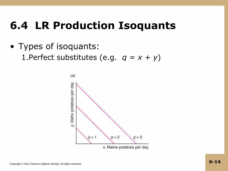
• Types of isoquants:

1.Perfect substitutes (e.g. q = x + y)




2.Fixed-proportions (e.g. q = min{g, b} )




3.Convex (e.g. q = L0.5K0.5 )


6.4 Substituting Inputs

• The slope of an isoquant shows the ability of a firm to replace one input with another (holding output constant).

• Marginal rate of technical substitution (MRTS) is the slope of an isoquant at a single point.

• MRTS tells us how many units of K the firm can replace with an extra unit of L (q constant)

• MPL = marginal product of labor; MPK = marginal product of capital

• Thus,


6.4 Substituting Inputs

• MRTS diminishes along a convex isoquant

• The more L the firm has, the harder it is to replace K with L.


6.4 Elasticity of Substitution

• Elasticity of substitution measures the ease with which a firm can substitute capital for labor.

• Can also be expressed as a logarithmic derivative:

• Example: CES production function,

Constant elasticity:



• How much does output change if a firm increases all its inputs proportionately?

• Production function exhibits constant returns to scale when a percentage increase in inputs is followed by the same percentage increase in output.

• Doubling inputs, doubles output f(2L, 2K) = 2f(L, K)

• More generally, a production function is homogeneous of degree γ if f(xL, xK) = xγf(L, K) where x is a positive

constant.



• Production function exhibits increasing returns to scale when a percentage increase in inputs is followed by a larger percentage increase in output.

• f(2L, 2K) > 2f(L, K)

• Occurs with greater specialization of L and K; one large plant more productive than two small plants

• Production function exhibits decreasing returns to scale when a percentage increase in inputs is followed by a smaller percentage increase in output.

• f(2L, 2K) < 2f(L, K)

• Occurs because of difficulty organizing and coordinating activities as firm size increases.


6.5 Varying Returns to Scale



• Even if all firms are producing efficiently (an assumption we make in this chapter), firms may not be equally productive.

• Relative productivity of a firm is the firm’s output as a percentage of the output that the most productive firm in the industry could have produced with the same inputs.

• Relative productivity depends upon:

1.Management skill/organization

2.Technical innovation

3.Union-mandated work rules

4.Work place discrimination

5.Government regulations or other industry restrictions

6.Degree of competition in the market



• An advance in firm knowledge that allows more output to be produced with the same level of inputs is called technical progress.

• Example: Nano by Tata Motors

• Neutral technical change involves more output using the same ratio of inputs.

• Non-neutral technical change involves altering the proportion in which inputs are used to produce more output.

• Organizational change may also alter the production function and increase output.

• Examples: automated production of Gillette razor blades, mass production of Ford automobiles

chapter 6 firms and production - bcit school of business...

Documents