54

CHAPTER 6

Beams:

Beams - structural members supporting

loads at various points along the member.

Transverse loadings of beams are

classified as concentrated loads or

distributed loads.

Applied loads result in internal forces

consisting of a shear force (from the

shear stress distribution) and a bending

couple (from the normal stress

distribution).

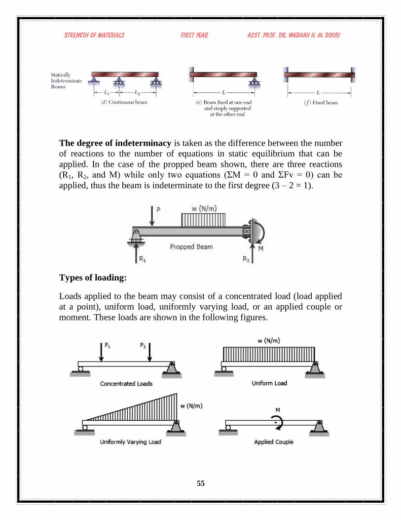
Classification of Beams:

1. Statically Determinate Beams:

Statically determinate beams are those beams in which the reactions of the

supports may be determined by the use of the equations of static equilibrium.

The beams shown below are examples of statically determinate beams.

2. Statically Indeterminate Beams:

If the number of reactions exerted upon a beam exceeds the number of

equations in static equilibrium, the beam is said to be statically

indeterminate. In order to solve the reactions of the beam, the static

equations must be supplemented by equations based upon the elastic

deformations of the beam.

55

The degree of indeterminacy is taken as the difference between the number

of reactions to the number of equations in static equilibrium that can be

applied. In the case of the propped beam shown, there are three reactions

(R1, R2, and M) while only two equations (ΣM = 0 and ΣFv = 0) can be

applied, thus the beam is indeterminate to the first degree (3 – 2 = 1).

Types of loading:

Loads applied to the beam may consist of a concentrated load (load applied

at a point), uniform load, uniformly varying load, or an applied couple or

moment. These loads are shown in the following figures.

56

Shear Force and Bending Moment Diagram:

The determination of the maximum absolute values of the shear and of

the bending moment in a beam are greatly facilitated if V and M are plotted

against the distance x measured from one end of the beam. Besides, as you

will see later, the knowledge of M as a function of x is essential to the

determination of the deflection of a beam.

In the examples and sample problems of this section, the shear and

bending-moment diagrams will be obtained by determining the values of V

and M at selected points of the beam. These values will be found in the usual

way, i.e., by passing a section through the point where they are to be

determined (Fig. a) and considering the equilibrium of the portion of beam

located on either side of the section (Fig. b). Since the shear forces V and V

have opposite senses, recording the shear at point C with an up or down

arrow would be meaningless, unless we indicated at the same time

which of the free bodies AC and CB we are considering.

For this reason, the shear V will be

recorded with a sign: a plus sign if

the shearing forces are directed as

shown in Fig.a, and a minus sign

otherwise. A similar convention will

apply for the bending moment M. It

will be considered as positive if the

bending couples are directed as

shown in that figure, and negative

otherwise. Summarizing the sign

conventions we have presented, we

state:

The shear V and the bending

moment M at a given point of

abeam are said to be positive when

the internal forces and couples

acting on each portion of the beam

are directed as shown in Fig. a.

57

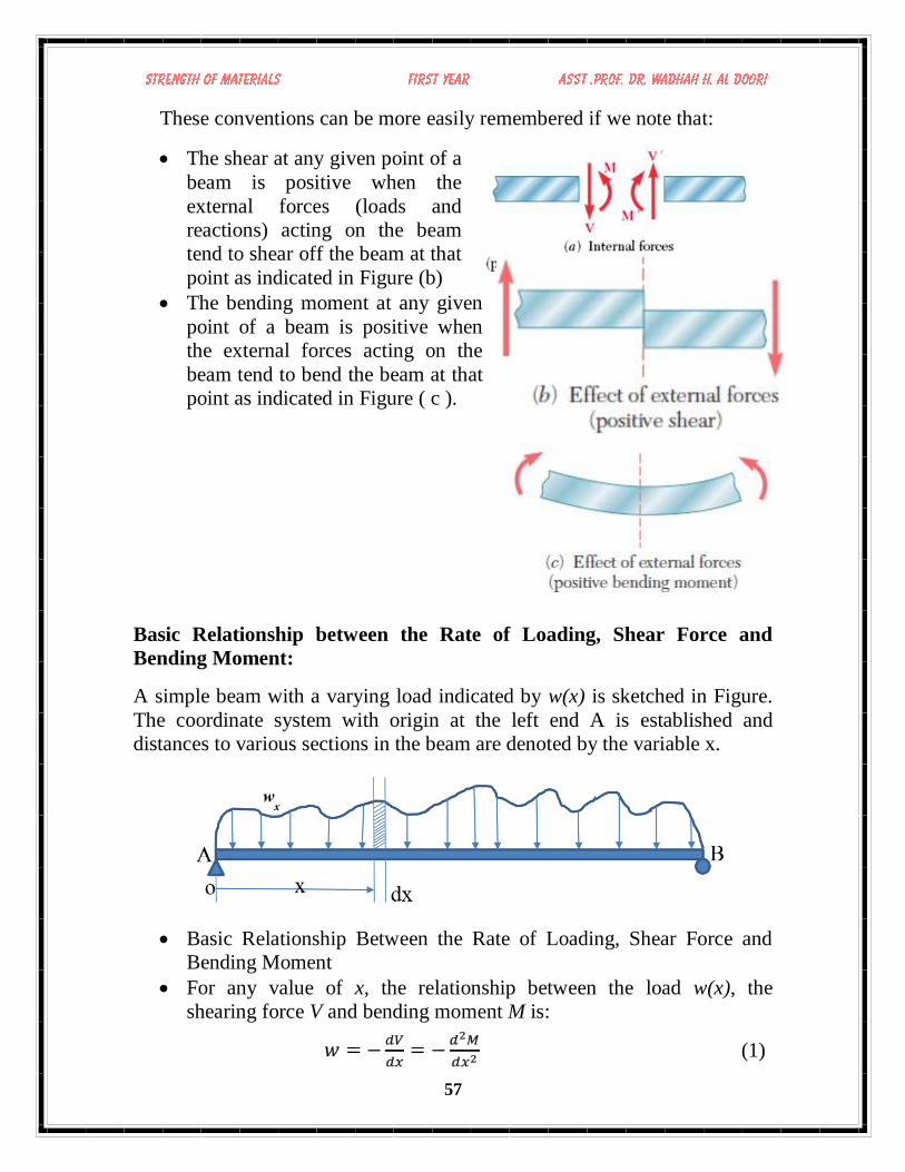
These conventions can be more easily remembered if we note that:

The shear at any given point of a

beam is positive when the

external forces (loads and

reactions) acting on the beam

tend to shear off the beam at that

point as indicated in Figure (b)

The bending moment at any given

point of a beam is positive when

the external forces acting on the

beam tend to bend the beam at that

point as indicated in Figure ( c ).

Basic Relationship between the Rate of Loading, Shear Force and

Bending Moment:

A simple beam with a varying load indicated by w(x) is sketched in Figure.

The coordinate system with origin at the left end A is established and

distances to various sections in the beam are denoted by the variable x.

Basic Relationship Between the Rate of Loading, Shear Force and

Bending Moment

For any value of x, the relationship between the load w(x), the

shearing force V and bending moment M is:

(1)

58

And for the relationship between shearing force V and bending

moment M is:

(2)

Conclusions: From the above relations, the following important

conclusions may be drawn:

From Equ. (2), the area of the shear force diagram between any two

points, from the basic calculus is the bending moment diagram.

The slope of bending moment diagram is the shear force, thus:

Thus, if V=0, the slope of the bending moment diagram is zero and the

bending moment is therefore constant.

The maximum or minimum bending moment occurs where

The slope of the shear force diagram is equal to the magnitude of the

intensity of the distributed loading at any position along the beam.

The ( -ve) sign is as a consequence of our particular choice of sign

conventions.

There are two methods to solve problems of shear and bending diagrams:

1) Method of Equations, and

2) Method of areas

59

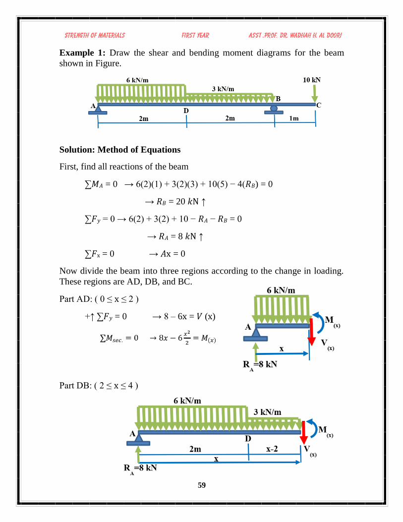
Example 1: Draw the shear and bending moment diagrams for the beam

shown in Figure.

Solution: Method of Equations

First, find all reactions of the beam

∑𝑀𝐴 = 0 → 6(2)(1) + 3(2)(3) + 10(5) − 4(𝑅𝐵) = 0

→ 𝑅𝐵 = 20 𝑘N ↑

∑𝐹𝑦 = 0 → 6(2) + 3(2) + 10 − 𝑅𝐴 − 𝑅𝐵 = 0

→ 𝑅𝐴 = 8 𝑘N ↑

∑𝐹x = 0 → 𝐴x = 0

Now divide the beam into three regions according to the change in loading.

These regions are AD, DB, and BC.

Part AD: ( 0 ≤ x ≤ 2 )

+↑ ∑𝐹𝑦 = 0 → 8 – 6x = 𝑉 (x)

Part DB: ( 2 ≤ x ≤ 4 )

60

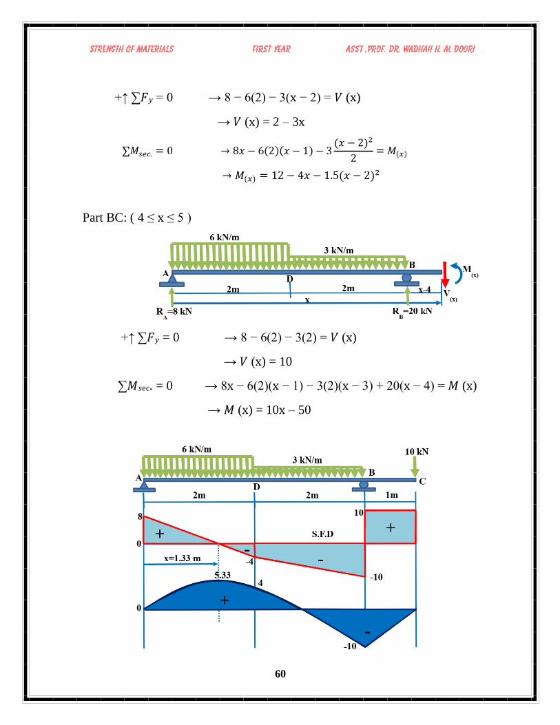
+↑ ∑𝐹𝑦 = 0 → 8 − 6(2) − 3(x − 2) = 𝑉 (x)

→ 𝑉 (x) = 2 – 3x

Part BC: ( 4 ≤ x ≤ 5 )

+↑ ∑𝐹𝑦 = 0 → 8 − 6(2) − 3(2) = 𝑉 (x)

→ 𝑉 (x) = 10

∑𝑀𝑠ec. = 0 → 8x − 6(2)(x − 1) − 3(2)(x − 3) + 20(x − 4) = 𝑀 (x)

→ 𝑀 (x) = 10x – 50

61

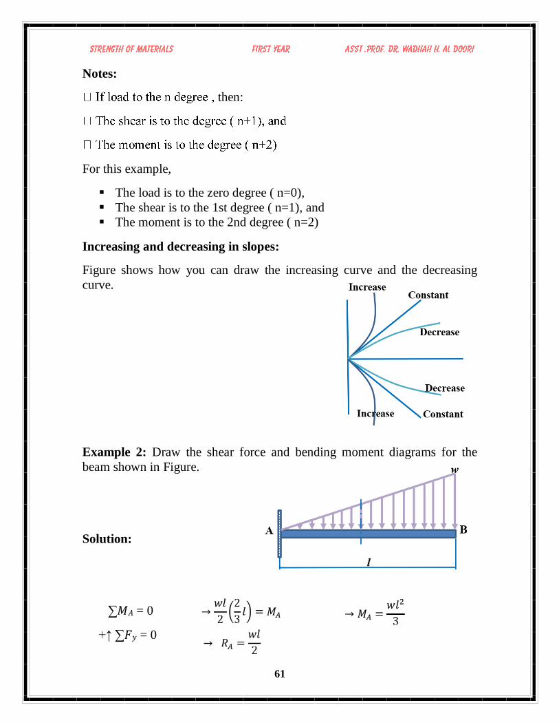
Notes:

then:

For this example,

The load is to the zero degree ( n=0),

The shear is to the 1st degree ( n=1), and

The moment is to the 2nd degree ( n=2)

Increasing and decreasing in slopes:

Figure shows how you can draw the increasing curve and the decreasing

curve.

Example 2: Draw the shear force and bending moment diagrams for the

beam shown in Figure.

Solution:

∑𝑀𝐴 = 0

+↑ ∑𝐹𝑦 = 0

62

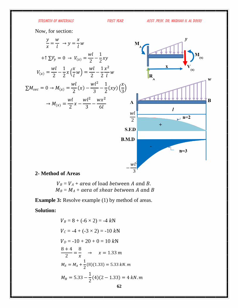
Now, for section:

2- Method of Areas

𝑉𝐵 = 𝑉𝐴 + 𝑎re𝑎 𝑜f load 𝑏e𝑡𝑤een 𝐴 𝑎nd 𝐵. 𝑀𝐵 = 𝑀𝐴 + 𝑎er𝑎 𝑜f 𝑠ℎe𝑎r 𝑏e𝑡𝑤een 𝐴 𝑎nd 𝐵

Example 3: Resolve example (1) by method of areas.

Solution:

𝑉𝐵 = 8 + (-6 × 2) = -4 𝑘N

𝑉𝐶 = -4 + (-3 × 2) = -10 𝑘N

𝑉𝐷 = -10 + 20 + 0 = 10 𝑘N

63

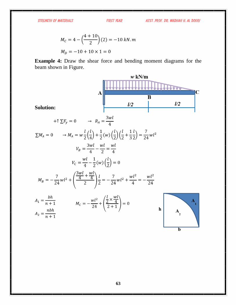
Example 4: Draw the shear force and bending moment diagrams for the

beam shown in Figure.

Solution:

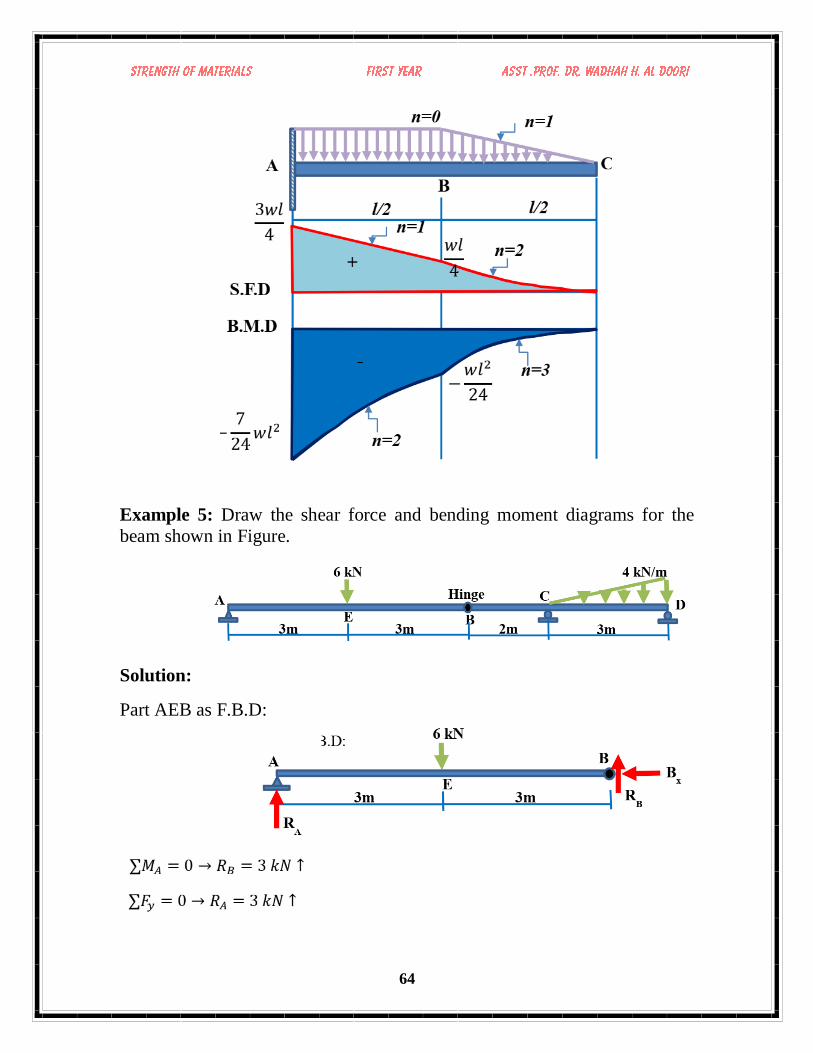
64

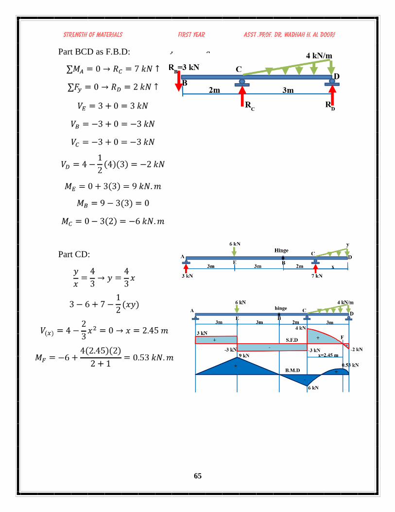
Example 5: Draw the shear force and bending moment diagrams for the

beam shown in Figure.

Solution:

Part AEB as F.B.D:

65

Part BCD as F.B.D:

Part CD:

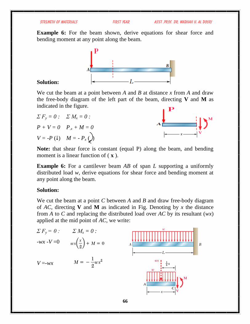
66

Example 6: For the beam shown, derive equations for shear force and

bending moment at any point along the beam.

Solution:

We cut the beam at a point between A and B at distance x from A and draw

the free-body diagram of the left part of the beam, directing V and M as

indicated in the figure.

Σ Fy = 0 : Σ Mx = 0 :

P + V = 0 P.x + M = 0

V = -P (↓) M = - Px ( )

Note: that shear force is constant (equal P) along the beam, and bending

moment is a linear function of ( x ).

Example 6: For a cantilever beam AB of span L supporting a uniformly

distributed load w, derive equations for shear force and bending moment at

any point along the beam.

Solution:

We cut the beam at a point C between A and B and draw free-body diagram

of AC, directing V and M as indicated in Fig. Denoting by x the distance

from A to C and replacing the distributed load over AC by its resultant (wx)

applied at the mid point of AC, we write:

Σ Fy = 0 : Σ Mx = 0 :

-wx -V =0

V =-wx

67

Example 7: For the simply supported beam AB of span L supporting a

single concentrated load P, derive equations for shear force and bending

moment at any point along the

beam.

Solution:

We first determine the reactions

at the supports from the free-body

diagram of the entire beam; we find that the magnitude of each reaction is

equal to P/2. Next we cut the beam

at a point D between A and C and

draw the free-body diagrams of AD

and DB. Assuming that shear and

bending moment are positive, we

direct the internal forces V and V’

and the internal couples M and M’

as indicated in Fig. Considering the

free body AD and writing that the

sum of the vertical components and

the sum of the moments about D of

the forces acting on the free body

are zero, we find:

V =+P/2 and M =+Px/2.

Both the shear and bending moment are therefore positive; this may be

checked by observing that the reaction at A tends to shear off and to bend the

beam at D as indicated in Figs. b and c. The shear has a constant value

V =P/2, while the bending moment increases linearly from M = 0 at x = 0 to

M =PL/4 at x =L/2.

Cutting, now, the beam at a point E between C and B and considering the

free body EB (Fig. c), we write that the sum of the vertical components and

68

the sum of the moments about E of the forces acting on the free body are

zero. We obtain:

V = - P/2 and M =P(L -x)/2.

The shear is therefore negative and the bending moment positive; this can be

checked by observing that the reaction at B bends the beam at E as indicated

in Fig. c but tends to shear it off in a manner opposite to that shown in Fig.b.

Note that the shear has a constant value V = -P/2 between C and B, while

the bending moment decreases linearly from M = PL/4 at x = L/2 to M = 0

at x = L.

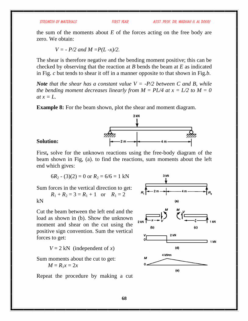
Example 8: For the beam shown, plot the shear and moment diagram.

Solution:

First, solve for the unknown reactions using the free-body diagram of the

beam shown in Fig, (a). to find the reactions, sum moments about the left

end which gives:

6R2 - (3)(2) = 0 or R2 = 6/6 = 1 kN

Sum forces in the vertical direction to get:

R1 + R2 = 3 = R1 + 1 or R1 = 2

kN

Cut the beam between the left end and the

load as shown in (b). Show the unknown

moment and shear on the cut using the

positive sign convention. Sum the vertical

forces to get:

V = 2 kN (independent of x)

Sum moments about the cut to get:

M = R1x = 2x

Repeat the procedure by making a cut

69

between the right end of the beam and the 3-kN load, as shown in (c). Again,

sum vertical forces and sum moments about the cut to get:

V = 1 kN (independent of x),

and M = 1x

The plots of these expressions for shear and moment give the shear and moment

diagrams (as shown in Fig.(d) and (e)

It should be noted that the shear diagram in this example has a jump at

the point of the load and that the jump is equal to the load. This is

always the case. Similarly, a moment diagram will have a jump equal

to an applied concentrated moment. In this example, there was no

concentrated moment applied, so the moment was everywhere

continuous.

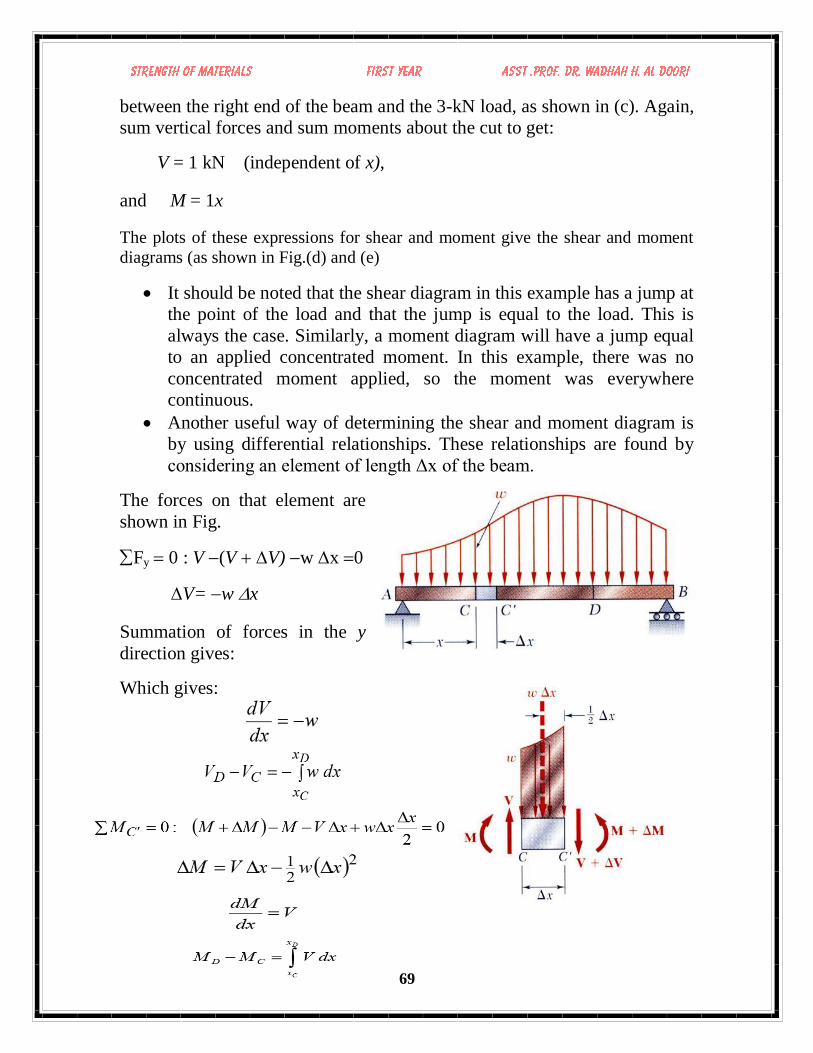
Another useful way of determining the shear and moment diagram is

by using differential relationships. These relationships are found by

considering an element of length Δx of the beam.

The forces on that element are

shown in Fig.

Fy 0 : V (V V) w x 0

V= w x

Summation of forces in the y

direction gives:

Which gives:

70