106

CHAPTER - 5

107

DEVELOPMENT OF MUTUAL INDUCTANCE TYPE

SODIUM LEVEL SENSOR WITH A NEW TEMPERATURE

COMPENSATION TECHNIQUE

5.1 INTRODUCTION

The under sodium ultrasonic viewing system efficiently functions only if the

components are adequately immersed in sodium pool. This is ensured using level measuring

system. Even though the traditional continuous level sensors used in small experimental

reactor is also of non contact type working on mutual inductance principle, for large power

reactors robust, longer length (~ 10 m) level probes are required. Hence, the third part of the

research work is targeted towards development of a long length level probe with application

focused towards PFBR. As the temperature gradient is more for longer probes, better

temperature compensation technique is required and a new temperature compensation

technique has been devised to improve the accuracy which also simplifies the electronics.

Detailed developmental activities in sensor, new temperature compensation technique,

studies to improve the sensitivity, its electronics and sodium testing results are discussed in

this chapter.

As already discussed in chapter-1, the primary and secondary circuits of FBR have a

large number of free liquid –sodium surfaces. Control of the relative level is important

during various conditions of the reactor operation. Hence, a large number of measurements

of high temperature sodium level sensors are required. As an alkali metal, sodium is highly

reactive with air and water and it is incompatible with many commonly used engineering

materials. In addition to the essential requirement of compatibility of the sensors used with

liquid sodium up to 823 K, the integrity of the system should be maintained even in the case

of breach of the sensor. So, conventional instrumentation devices cannot be readily used in

sodium systems. The above requirements necessitate specially developed sensors for use in

108

liquid sodium. The characteristics required for level sensors include (i) wide and high

operating temperature with simple temperature compensation technique, (ii) should be of non

contact type with minimum weld joints, (iii) should not depend on wetting effects and (iv)

should be robust and withstand cross flow during normal operation. Operationally the levels

at the pool region and secondary circuit must be measured continuously to find the gross

sodium hold up in the primary circuit, to ensure that an adequate level is maintained at the

heat exchanger inlet to prevent vortex and gas entrainment and also to monitor entry of

secondary sodium into primary sodium. The typical installations of level sensors in PFBR is

shown in Fig. 5.1

Fig. 5.1 Typical Installation of Level sensors in PFBR (LS-Discontinuous level probe,

LW- Continuous level probe) (Safety Report on PFBR)

109

Discontinuous level measurement is needed to guard against any gross loss of coolant from

the system. It is used for safety purposes and also provides redundancy. Typical discrete

level sensors works on the principle of step change in resistance when sodium touches the

sensing portion. The major disadvantages of this system include (i) poor wettability at low

temperature (200°C) and (ii) effect of vapor deposition on probe surface. To overcome these

problems, non contact, mutual inductance type discontinuous level sensors are essential.

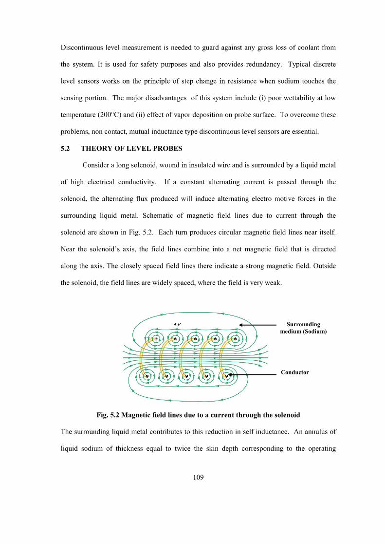
5.2 THEORY OF LEVEL PROBES

Consider a long solenoid, wound in insulated wire and is surrounded by a liquid metal

of high electrical conductivity. If a constant alternating current is passed through the

solenoid, the alternating flux produced will induce alternating electro motive forces in the

surrounding liquid metal. Schematic of magnetic field lines due to current through the

solenoid are shown in Fig. 5.2. Each turn produces circular magnetic field lines near itself.

Near the solenoid’s axis, the field lines combine into a net magnetic field that is directed

along the axis. The closely spaced field lines there indicate a strong magnetic field. Outside

the solenoid, the field lines are widely spaced, where the field is very weak.

Fig. 5.2 Magnetic field lines due to a current through the solenoid

The surrounding liquid metal contributes to this reduction in self inductance. An annulus of

liquid sodium of thickness equal to twice the skin depth corresponding to the operating

Conductor

Surrounding medium (Sodium)

110

frequency, is virtually equivalent to an infinite sea of sodium (Mcgonigal, 1971). The change

in self inductance is proportional to the depth of immersion. The measurement of self

inductance of the coil is hampered by the series resistance of the winding. When the series

resistance is high and the self inductance is low, the measurement becomes very difficult and

inaccurate. To overcome this, bifilar coil system is used, where the effect may be regarded as

change of mutual inductance between the two coils. When alternating constant current is fed

into primary coil, e.m.f. induced in the secondary does not depend on resistances of the coils.

It depends only on coefficient of coupling and the magnitude of eddy currents produced in

the surrounding medium. Change of inductance is caused by eddy currents which produce a

magnetic field in opposition to that produced by the primary current in the coil. The

penetration of these eddy currents into the surrounding conducting medium is a function of

the resistivity of the medium and the frequency of input current. Expressions for mutual

inductance (M) and e.m.f induced in secondary coils (e) are given below.

2

0 r 1 2N N r

Ml

------------------------------------------------------------------ (5.1)

d Ie -M

d t --------------------------------------------------------------------------- (5.2)

1 2M k L L -------------------------------------------------------------------------- (5.3)

Where k is the coupling factor, for loosely wounded windings k 1

1L self inductance of primary coil

2L self inductance of secondary coil

M mutual inductance between coils

111

The induced magnetic vector potential at (r, z) (Nestor, 1979) produced by a driving coil with

a fixed alternating current in solenoid coil is given below.

1 2 0 1 12 1 1 1 23

2 1 2 1 0

1( , ) I nA ( r,z ) I r ,r * I r * sin z l sin z l

( r r )( l l )

2 1

2 1 1 22

z l z lJ r ,r J r e e d

-------------------- (5.4)

1r Inner radius of coil

2r Outer radius of coil

1l Distance from bottom of coils to z = 0 plane

2l Distance from top of coils to z = 0 plane

l = 2 1( l l ) Coil length

1n Number of primary coil turns

2n Number of secondary coil turns

1I Primary exciting current

0 Free space permeability

Separation constant

z Transfer impedance

Angular frequency of 1I

Alternating magnetic field produced by current in primary coil along with magnetic field

produced by eddy currents generated in surrounding electrically conducting mediums led to

generation of e.m.f in secondary coil. E.m.f induced in secondary coil is given below.

2 12 21 2 1 02 2 1 2 1 2 1 2 12 2 6

2 1 2 1 0

2 12 1 1( l l )j n n I

V I r ,r cos ( l l ) J r ,r ( l l ) e d( r r ) ( l l )

------------------------(5.5)

112

5.3 PRINCIPLE OF OPERATION

The Mutual Inductance type Level Probe (MILP) works on the principle of variation

of mutual inductance between two windings when they are in the proximity of an electrically

conducting fluid such as sodium. The MILP has two windings wound in bifilar fashion on a

non-magnetic stainless steel former. The probe is inserted in a stainless steel pocket. The

primary winding of the probe is excited with an AC constant current at a constant frequency.

Due to mutual inductance, an electro motive force is induced in the secondary coil. The

liquid sodium surrounding the probe acts as a short-circuited winding, because sodium is a

good electrical conductor. An electro motive force will be induced in sodium also and the

eddy current flows in it. The magnetic flux due to eddy current will oppose the main flux

produced by the primary winding. Hence, the net flux linked with secondary decreases and

thereby the secondary voltage reduces when the sodium level increases. The secondary

voltage is an inverse linear function of the sodium level. When the sodium temperature

increases, the resistivity of sodium increases. Hence, the eddy current decreases and the

induced voltage in secondary coil increases. So, temperature compensation is required in

order to make the output voltage independent of temperature.

5.4 CONSTRUCTION OF LONG LENGTH LEVEL PROBE

The sensor consists of sensing element called bobbin and pocket. Traditional level

probes R have short active lengths (2.5 m). As long length level probes are required for large

power reactors, free insertion and withdrawal of the bobbin into the pocket is required.

Therefore, the radial clearance between pocket and bobbin has to be liberal. For the present

purpose, a standard pipe of size 1¼” SCH10 (42.16 mm OD, 36.62 mm ID) as pocket and 28

mm diameter bobbin are selected. From the practical point of view, the measurement of the

self inductance of a coil is hampered by the series resistance of the windings. To overcome

this difficulty bifilar coil system is used.

113

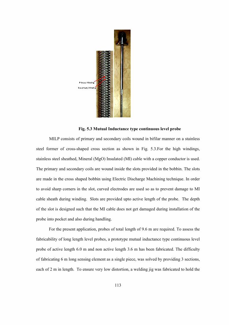
Fig. 5.3 Mutual Inductance type continuous level probe

MILP consists of primary and secondary coils wound in bifilar manner on a stainless

steel former of cross-shaped cross section as shown in Fig. 5.3.For the high windings,

stainless steel sheathed, Mineral (MgO) Insulated (MI) cable with a copper conductor is used.

The primary and secondary coils are wound inside the slots provided in the bobbin. The slots

are made in the cross shaped bobbin using Electric Discharge Machining technique. In order

to avoid sharp corners in the slot, curved electrodes are used so as to prevent damage to MI

cable sheath during winding. Slots are provided upto active length of the probe. The depth

of the slot is designed such that the MI cable does not get damaged during installation of the

probe into pocket and also during handling.

For the present application, probes of total length of 9.6 m are required. To assess the

fabricability of long length level probes, a prototype mutual inductance type continuous level

probe of active length 6.0 m and non active length 3.6 m has been fabricated. The difficulty

of fabricating 6 m long sensing element as a single piece, was solved by providing 3 sections,

each of 2 m in length. To ensure very low distortion, a welding jig was fabricated to hold the

114

bend strips in position for laser welding which was also used for joining the 2 m sections to

form 6 m bobbin. Special fixtures and a dedicated winding table with rotary holders were

fabricated to hold the bobbin while winding the MI cable. For making a long pocket long

welding table was fabricated using machined aluminum plate and V blocks. The long tubes

were straightened using hydraulic/screw press and finally the straightness of +/- 1 mm per

meter was achieved. The robust and long length level probe has been fabricated successfully.

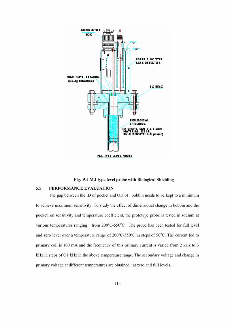
Further, provision has also been made in the pocket to detect the sodium leak using

spark plug type leak detector. Leak tight arrangement is achieved using Lip-seal welding,

instead of O-ring arrangement due to high temperature. A stainless steel ring with bolt-nut

arrangement is used to avoid load on Lip seal welding. To provide biological shielding, SS

balls were used instead of stainless steel blocks for free insertion of MI cable as shown in

Fig.5.4. In order to provide leak tightness, MI cable is brazed with stainless steel flange

using high temperature brazing alloy. For this, a number of mockups have been carried out

successfully to study the fabrication feasibility, as the MI cables are fragile and brazing them

to stainless steel flange without affecting the thin copper conductor inside posed a major

challenge.

115

Fig. 5.4 M.I type level probe with Biological Shielding

5.5 PERFORMANCE EVALUATION

The gap between the ID of pocket and OD of bobbin needs to be kept to a minimum

to achieve maximum sensitivity. To study the effect of dimensional change in bobbin and the

pocket, on sensitivity and temperature coefficient, the prototype probe is tested in sodium at

various temperatures ranging from 200oC-550oC. The probe has been tested for full level

and zero level over a temperature range of 200oC-550oC in steps of 50oC. The current fed to

primary coil is 100 mA and the frequency of this primary current is varied from 2 kHz to 3

kHz in steps of 0.1 kHz in the above temperature range. The secondary voltage and change in

primary voltage at different temperatures are obtained at zero and full levels.

116

% S VS FREQUENCY

18.000

18.500

19.000

19.500

20.000

20.500

21.000

21.500

2.0 2.1 2.2 2.3 2.4 2.5 2.6 2.7 2.8 2.9 3.0

FREQUENCY(kHz)

% S

200C

250C300C350C400C450C550C

Fig. 5.5 % Sensitivity Vs frequency

Using the data a plot is obtained between frequency and % sensitivity (%S) and is

shown in Fig. 5.5, where sensitivity is defined by,

Zero level secondary voltage Full level Secondary voltage%S

Zero level Secondary vo

x

l g

10

e

0

ta

It has been found that 2.5 kHz is the optimum excitation frequency to minimize the effect of

temperature on the output. The graph shows a crossover at a particular frequency which is

due to variation in flux pattern of sodium surrounding the pocket at higher frequencies.

Change in the secondary output voltage due to change in level (zero to full) is around 20%

and is sufficient enough to adjust in electronics.

5.6 DEVELOPMENT ON TEMPERATURE COMPENSATION TECHNIQUE

The probe secondary voltage is a function of sodium level as well as temperature. To

find out the actual sodium level using MI probe, effect of temperature on secondary output of

117

the level probe has to be eliminated. The temperature compensation technique is complicated

because of the facts, (i) Electrical conductivities of sodium and stainless steel vary with

temperature at different rate, (ii) Temperature coefficient for the sensor uncovered and fully

covered with sodium is different, (iii) mutual inductance at both the sodium uncovered and

fully covered states increases with increasing temperature but at different rates as shown in

Fig. 5.6, and (iv) temperature distribution in the direction of length of the probe cannot be

determined because it depends on sodium temperature, sodium level, and temperature at the

top of the probe and cover gas temperature (Kuniji, 1975).

Fig. 5.6 Electrical conductivities of sodium and stainless steel

Temperature in (ºC)

Con

du

ctiv

ity

in (

mh

o/m

)

Stainless steel

Sodium

118

Fig. 5.7 Earlier method of temperature compensation

A basic temperature compensation can be achieved by measuring the primary voltage

variation, which is a measure of average temperature of the probe. This method of

temperature correction achieved through electronics is shown in Fig. 5.7. The procedure for

calibration of electronics is, at the lowest operating temperature the electronics is adjusted for

zero level and full level by adjusting gain of an amplifier. At the highest operating

temperature, only at full level the temperature compensation amplifier is adjusted to show full

level reading. Hence, adjustments are carried out only for full level at two extreme

temperatures and this method of temperature compensation is partial. This contributes to an

error of +/- 3% of span.

119

5.6.1 Principle of new temperature compensation Technique

This method utilizes the internal resistance variation of the coil with temperature and

uses variation of internal resistance as a correction factor to compensate temperature effect.

In the case of any given level, the internal resistance of the secondary coil increases with

temperature. By connecting an external resistance, Rext, there is a current flow such that the

voltage drop within the internal resistance of the probe compensating the increase in the

voltage induced within the secondary (Paris et al., 1976). Schematic of the circuit is shown in

Fig. 5.8.

Fig. 5.8 Schematic of continuous Level probe

In Fig. 5.8, E denotes induced voltage in secondary, Ri denotes internal resistance of

secondary, i is the circulating current and Rext is the external resistance to be added for

temperature compensation. Equation of the circuit in respect of a fixed level of sodium is as

follows

extext

ext i

R x EE’ R i

Rx

R

---------------------------------------------------------------(5.6)

When the temperature varies, the voltage at the terminals of the extR varies by dE’ , Which is

given by:

120

ext ext

i2ext i ext i

R E ExR E’ R

R R R R

x

---------------------------------------------------(5.7)

This variation should be reduced to zero (i.e.) E’ = 0;

Applying this condition to eqn (5.7) we get, iext i

Ex R R R

E

----------------(5.8)

Eqn (5.8) can be written as, iext i

E´x RR R

E

Where,

iR = Internal resistance calculated by dividing primary voltage by primary current

E = Secondary output

Rext = External resistance

iR = Difference in internal resistance at extreme temperature

∆E = Difference in secondary voltage at extreme temperature.

For this calculation, primary resistance is considered as internal resistance of the

secondary coil since the winding is bifilar. It is known that secondary output voltage is a

function of sodium level, temperature and also the frequency of excitation. Equation 5.3 gives

the value of external resistance, which takes care of temperature compensation. Effect of

frequency on secondary output is obtained by plotting the value of external resistance and

frequency for zero sodium level and full sodium level. The intersection point of these two

curves gives value of external resistance for optimum frequency.

5.6.2. Experimental Validation

The prototype MI level probe is tested in sodium for implementing new method of

temperature compensation technique. At different frequencies the data was collected in

sodium for extreme temperature at zero and full level of sodium. The thermocouple measures

121

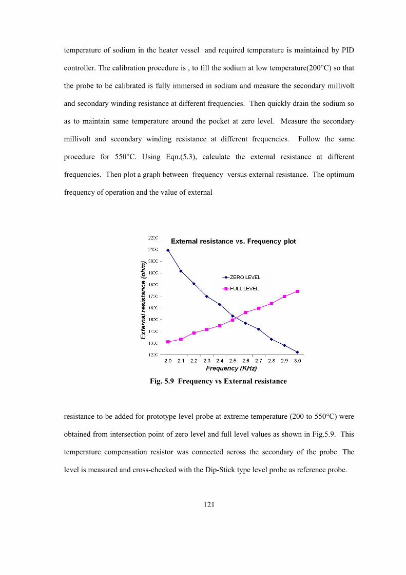
temperature of sodium in the heater vessel and required temperature is maintained by PID

controller. The calibration procedure is , to fill the sodium at low temperature(200°C) so that

the probe to be calibrated is fully immersed in sodium and measure the secondary millivolt

and secondary winding resistance at different frequencies. Then quickly drain the sodium so

as to maintain same temperature around the pocket at zero level. Measure the secondary

millivolt and secondary winding resistance at different frequencies. Follow the same

procedure for 550°C. Using Eqn.(5.3), calculate the external resistance at different

frequencies. Then plot a graph between frequency versus external resistance. The optimum

frequency of operation and the value of external

Fig. 5.9 Frequency vs External resistance

resistance to be added for prototype level probe at extreme temperature (200 to 550°C) were

obtained from intersection point of zero level and full level values as shown in Fig.5.9. This

temperature compensation resistor was connected across the secondary of the probe. The

level is measured and cross-checked with the Dip-Stick type level probe as reference probe.

122

Table-5.1 Secondary output for different temperature with compensation using external resistor

ΔE :Change in secondary O/P from zero level to full level in mV at a particular temperature. ΔE_T : Change in secondary O/P in mV w.r.t temperature.

Change in secondary O / P from zero level to full level in mV Sensitivity

Active length of the probe

% S : % Variation of secondary O/P w.r.t level change at a given temperature

: Change in secondary O / P E

Secondary O / P at zero leve

( )0

lx10

Change in secondary O / P w.r.t temperature mV Error in level

Sensitivity mV( )/ mm

o o

% Sec.voltage variation w.r.t e _ ave E _ T

E _ Ave for temperature from 200 C 550 C

Secondary output (mV) Sodium

level (mm) 2200 C 3500 C 4500 C 5500 C

ΔE_T

Error in level (mm)

% Sec.voltage variation w.r.t

Δe_ave for temp. from 200 oC-550

oC 0

146.89 147.05 146.8 146.66 0.39 78 1.33

6000

117.56 117.6 117.35 117.3 0.3 60 1.02

ΔE

29.33 29.45 29.45 29.36 ΔE_Ave = 29.40

%S 19.97 20.03 20.06 20.02

%S_Ave = 20.02

Drop across primary (V)

4.759

6.299

7.317

8.453

Zero Level

Drop across primary (V)

4.748

6.143

7.12

8.134

Full Level

123

120

125

130

135

140

145

150

155

160

0

1200

2400

3600

4800

6000

Sodium level/(mm)

Sec.o

utp

ut/

(mV

)

220C

350C

450C

550C

Fig. 5.10 Secondary output without temperature compensation

110

115

120

125

130

135

140

145

150

0 1000 2000 3000 4000 5000 6000

Sodium level (mm)

Seco

nd

ary

ou

tpu

t (m

v)

Fig. 5.11 Secondary output with temperature compensation using external resistor

124

Fig. 5.12 Level measuring system using new method of temperature compensation

Figure 5.10 shows the secondary millivolt versus level without temperature

compensation. The procedure used is for various sodium temperatures and at different levels

the secondary millivolt is measured by quickly draining the sodium so as to maintain constant

temperature along the level probe. This experiment is carried out to assess the linearity of the

probe at various levels at a uniform temperature. After connecting the resistance across the

secondary, the graph between actual level and secondary millivolt with temperature

compensation is plotted as shown in Fig. 5.11. The same quick draining procedure for

maintaining the uniform temperature throughout the pocket is followed to obtain the graph.

125

To simulate the actual condition, for constant sodium temperature, at various sodium

levels, the secondary millivolt is measured after stabilization of cover gas and sodium

temperature. In this case, secondary millivolt is found to be independent of temperature. The

schematic of the level measuring system with new temperature compensation is shown in Fig.

5.12. Another interesting fact observed is at different temperature ranges, the value of

resistance as well as frequency of operation also changes. Table-5.2 below shows the

different temperature ranges and the value of external resistance to be added.

Table-5.2 Variation of frequency and resistance at different temperature ranges

5.7 IMPROVED ELECTRONICS CHASSIS

The electronic chassis consists of two independent chains as shown in Fig. 5.13.

- an input chain

- an output chain.

The input chain feeds the primary winding of the probe with constant current and

constant frequency. The output chain consists of receiver circuit. The isolated AC signal of

secondary winding (5 mV to 250 mV) is processed by this circuit.

The exciter module has sinusoidal oscillator and a constant current drive circuit. The

clock is derived from the crystal oscillator and using hardware based Direct Digital

Synthesizer, the frequency of range 1 kHz to 10 kHz is selected with the resolution of 1 Hz.

Actual Value Temperature

range(ºC) Freq. (kHz)

Resistance (Ω)

200-550 2.47 1535

250-550 2.54 1600

300-550 2.57 1640

350-550 2.57 1790

400-550 2.57 1980

450-550 2.47 2450

200-300 2.28 1290

200-400 2.42 1300

126

As the signal level in the sensor is low of the order of few millivolts and the sensitivity is as

low as 20%, a stringent requirement of sine wave of low distortion and amplitude stability is

required in the electronics. The constant current source provides 0 to 200 mA rms isolated

current, able to drive 150 Ohms with current stability better than ± 0.05 %. Isolation

amplifier couple the sensor to both the energizing oscillator and the measuring unit to avoid

earth loops and interfering pick up signals. As the resistor is connected across the secondary

of the probe for providing temperature compensation, isolation amplifier with high input

impedance is used to avoid the loading effect. The receiver module is having an active band

pass filter in the range of 1 kHz to 5 kHz. In-situ test buttons shall be provided to increase /

decrease the probe current at front to check the healthiness of the probe as well as the

electronics. The receiver module has isolated input AC signal amplifier and isolated DC

output. The following are the parameters of receiver:

Input signal range : AC signal, 5 mV to 250 mV rms.

Input impedance : >105 ohms in the frequency band of 1 kHz to 5 kHz

Band width : Lower 3 db point – less than 1 kHz

Upper 3 db point – greater than 5 kHz

Stability : 50ppm/°C for ambient variation of 10 to 50°C

Linearity : better than ±0.2% of full scale

Output : 0 – 10V DC, 10 mA, isolated.

Trim pots for Zero & Span indication is provided at the front. High and low set points

are provided as trip contacts. The level reading is indicated in 1 mm resolution with 0.01%

of reading.

127

Fig. 5.13 Improved electronics for continuous level probe

5.8 STUDIES TO IMPROVE THE SENSITIVITY OF THE PROBE

The sensitivity of the level probe can be increased by increasing the number of

turns of the windings per unit length or increasing the coil winding diameter. Two bobbins of

varying diameters of 30 mm and 32 mm were fabricated and tested in sodium for obtaining

the sensitivity using new temperature compensation technique. All the three bobbin diameters

28 mm, 30 mm and 32 mm are tested in sodium in the same pocket of dimension 42.6 mm

OD/36 mm ID. As there is 10% variation in pocket dimensions are expected, to eliminate this

effect, levels probes are tested in the same pocket one after the other. The secondary mill volt

was measured at two extreme operating temperatures from 200 to 550°C. Using the proposed

temperature compensation technique, the sensitivity of 3 different probes are found out.

From the experimental result it is found that for 32 mm bobbin diameter probe, the sensitivity

is 26.5 % which is much better than the 28 mm bobbin diameter probe. Table-5.4 shows the

experimental results. Further, 32 mm diameter bobbin probe is easily insertable up to 10 m

pocket.

128

Table-5.3 Sensitivity studies for varying bobbin dimension

Particulars 28 mm bobbin size

level probe 30 mm bobbin size

level probe 32 mm bobbin size level probe

Frequency in kHz 2.25 2.35 2.55

External resistance Rext in Ω

214.6 161 154.46

Sensitivity in % 19.66 23.137 26.50

Radial gap 4.31 3.31 2.31

% Accuracy 0.4 0.8 0.9

5.9 DISCUSSION ON RESULTS

The proposed temperature compensation technique has been validated experimentally

for prototype MI type continuous level probe. The method of calculating external resistance

with minimum sodium data is established. Using this method, the temperature effect on level

is reduced from 10.59% to 1.5% over an extreme temperature without change in sensitivity of

the probe. The sensitivity of the probe is around 20% which is sufficient enough to adjust in

the electronics. The linearity of the probe is determined to be 0.7%. This technique not only

improves the accuracy to 1.5% , but also simplifies the electronic circuitry by eliminating the

temperature compensation circuitry. Another interesting fact to be observed is at different

temperature ranges, the value of resistance as well as frequency of operation also changes. A

comparison of performances of a partial compensation probe against the resistor compensated

probe is presented in Table 5.5. It is found that when the new method of temperature

compensation is applied to short length probe, the optimum frequency increased to 4.6 kHz

with an accuracy of 0.6 %. Studies have been made to improve the sensitivity of long length

probe by changing the bobbin diameter. The sensitivity improves from 26.5% to 20%.

129

Table-5.4 Results of partial compensation and resistor compensation probe

Parameter Partial

compensation probe

External resistor

compensation probe

Bobbin size 28 28

Pocket OD-34 mm/ ID-30mm OD-42.6mm/ ID-36mm

Wall thickness of pocket 2 mm 2.7 mm

Radial gap between bobbin and

pocket

1 mm 3 mm

Accuracy 3 % 1.5 %

Sensitivity 30 % 20 %

Active Length 2500 mm 9000 mm

Operating frequency 2.73 kHz 2.5 kHz

5.10 MI TYPE DISCRETE LEVEL PROBE

The MI type level sensor has certain advantages over the resistance-type level

detector. The MI type sensor works on non-contact principle whereas the resistance type

sensor works based on its contact with sodium. Besides, MI type is kept in a well or pocket,

and so maintenance of the sensor becomes easy. Also, the level sensor is not required to be

mounted in the vessel at the time of integrity test of the vessel after fabrication at the

manufacturer’s shop. Further, non-wetting of sodium with senor does not affect the operation

of MI type sensor. Considering the above advantages of MI type sensor, a prototype discrete

level sensor was fabricated with 5 discrete levels (1000 mm active length and 1000mm non

active length) and then tested in sodium. The bobbin diameter chosen for this application is

32 mm and located inside a pocket made of a standard pipe of (42.16 mm OD, 36.62 mm ID).

The probe is tested in sodium and studies conducted on frequency response of probe.

130

5.11 CONSTRUCTION OF MI TYPE DISCRETE LEVEL PROBE

The sensing part of the probe consists of one primary winding and two layers of

secondary windings as shown in Fig. 5.14. Bobbin is made of stainless steel former. The

primary and secondary coils are wound at different positions where sensing is required. The

primary winding of the bobbins are connected in series and secondary windings are

individual as shown in Fig. 5.15. The primary and secondary windings are wound with 1 mm

diameter mineral insulated cable with copper conductor. The probe is inserted in a stainless

steel pocket. The primary is excited with a constant AC current at a fixed frequency. When

the sodium surrounds the bobbin, induced signal in that bobbin secondary is minimal. When

there is no sodium around the bobbin the induced signal in secondary is the maximum. The

change in the induced signal of the secondary is utilized for sodium level detection. Since the

Fig. 5.14 Bobbin and windings of MI discrete level probe

coil lengths are much smaller (~ 20mm) compared to those used in the continuous type, the

effect of sodium temperature coefficient on the level detection is negligible. For the same

reason, the electronics is also made simpler.

131

Fig. 5.15 Schematic of MI discrete level sensor

5.12 FREQUENCY RESPONSE STUDIES

Experiment has been conducted by exciting the primary coil with an AC constant

current of 100 mA. Initially frequency response studies are carried out in sodium by varying

the frequency of the primary current from 2 kHz to 5 kHz in steps of 0.5 kHz and the results

are recorded. A graph is plotted between % Sensitivity vs Frequency. The plot is shown in

Fig. 5.16. From the graph it is found that at a frequency of 2.5 kHz, the percentage variation

of secondary output is almost constant for different temperature values.

132

%S Vs Frequency (kHz)

0

2

4

6

8

10

12

14

16

18

2 2.5 3 3.5 4 4.5 5

Frequency (kHz)

%S

150C

250C

350C

450C

550C

Fig. 5.16 %Sensitivity Vs Frequency (kHz)

5.13 DISCUSSION ON RESULT

From the experiments, it is found that due to temperature effect, the detection

accuracy is around 6 mm from the centre of the bobbin. A value between minimum value of

secondary output at bobbin immersed in sodium and maximum value of secondary output at

bobbin in argon has been chosen as threshold value. Even though the threshold voltage is

same for all the bobbins, each one triggers at different level due to sodium temperature

variations as well as ±1 turn variation in coil windings.

5.14 CLOSURE

As commercially available level sensors cannot be used in hostile sodium

environment, these sensors and instrumentation are specially designed based on mutual

inductance type. The present invention is directed to a level measuring probe which is easy

to use, has improved accuracy of measurement and provides an indication of level which is

almost independent of the temperature of the liquid in which the probe is immersed. For

large power reactors, long length level probe of active length 6 m and non active length of 3.6

133

m has been developed and tested in sodium to assess the sensitivity. A new temperature

compensation technique employing external resistor has also been developed. This technique

reduces the temperature effect on level from 10.59 % to 1.5 % over a wide temperature

range of 200°C to 550°C without change in sensitivity of the probe. Using this method, the

optimum frequency of excitation and the external resistance to be connected across the

secondary coil have been determined simultaneously. The sensitivity of the long length level

probe is estimated as 20 % around the operating frequency with an accuracy of 1.5 %. This

technique not only improves the accuracy but also simplifies the electronic circuitry by

eliminating the temperature compensation circuit. The linearity of the probe was found to be

0.7 % at different temperatures.

Studies have also been carried out to improve the sensitivity of the probe by varying

the coil diameter in the range of 28-32 mm. The sensitivity of 32mm diameter bobbin has

improved to 26.5 %. The radial gap is sufficient enough for easy insertion and withdrawal of

the probe into the pocket of length 10 m.

A prototype MI type discrete level probe with 5 levels have been fabricated with 32

mm diameter bobbin and tested for its performance in sodium at different temperature. The

operating frequency is determined to be 2.5 kHz where the temperature effect on secondary

millivolt is minimum. The discontinuous level detection accuracy is ± 6 mm around the

centre of the bobbin.

After successful development of prototype MI type continuous and discrete level

probes, 29 nos of Continuous and discrete level probes of each have been fabricated for use

in PFBR. The active length of the continuous level probe varies from 660 mm to 9300 mm.

These level probes were characterized in sodium for obtaining optimum frequency of

operation and external temperature compensation resistor.