chapter 5: photospheric elemental abundances - edocs · pdf filechapter 5: photospheric...
TRANSCRIPT
91
Chapter 5: Photospheric Elemental Abundances
5.1 Introduction
Photospheric abundances provide another means to help divide the stars in the
sample of study into three categories: main sequence stars ejected from the disk, low
mass evolved stars, or massive stars formed in situ in the halo. Population I stars that
have been ejected from the disk should show relative abundances which are consistent
with those observed in their parent population, represented by a control sample of
nearby Population I B stars. Unlike massive runaway main sequence stars, low mass
evolved stars should have abundances with enhancements or depletions of specific
elements due to mixing of processed material into their atmospheres or lowering of
abundances by grain formation over the course of their evolution. Lastly, stars which
formed in situ in the halo should have abundances which are significantly metal
deficient compared to the control sample of nearby Population I B stars.
Most sub luminous evolved stars in the sample are probably helium burning blue
horizontal branch (BHB) stars. These stars have completed their hydrogen burning
main sequence, climbed the red giant branch, and descended onto the blue end of the
horizontal branch. This track takes these stars though several episodes of mixing and
mass loss which affect the composition of their outer layers. Material that was
processed in the interior of the star during a previous stage of evolution has been mixed
into its photosphere causing enhancements and depletions of elements in specific
patterns. Products of partial CNO processing should be prominent in horizontal branch

92
stars as an enhancement of nitrogen and depletion of carbon with respect to oxygen. In
some cases, they may also have a higher helium abundance.
Unfortunately, this enhancement pattern is not completely unique to horizontal
branch stars. Massive main sequence B stars may undergo some mixing between their
photospheres and cores which would also bring products of the partial CNO process to
the surface while the star is still in its hydrogen burning phase. OBC and OBN stars are
otherwise normal main sequence O and B stars that have significant enhancements of
carbon and nitrogen in their photospheres.
External pollution of the photosphere of a main sequence star can also happen
when processed material from an evolved companion is deposited in the outer layers of
a star. The stars ejected by the binary supernova scenario (BSS) come from binary
systems where one star underwent a supernova explosion. Some amount of the material
from the supernova will find its way into the ejected companion’s atmosphere
(Portegies Zart 2000). Again in this case, enhancements are expected to fit the pattern
of the partial CNO process but there could also be enhancements as a result of s-
process, r-process, triple-α, and other nuclear processes in Type II supernova.
Luck (1993) presented a review of the abundance patterns observed in Post-
Asymptotic Giant Branch (PAGB) and Proto-Planetary Nebula (PPN) stars. PAGB and
PPN stars have evolved off the horizontal branch, up the asymptotic giant branch
(AGB), and to their present position on the HR diagram. As a result, these stars show
the effects of several mixing and mass loss episodes beyond those expected for
horizontal branch stars. The abundance patterns observed in these stars have been
altered by the same processes which affect the composition of BHB stars plus other

93
processes such as triple-α helium burning. Intuitively one might conclude that the
triple-α process enhances carbon, however in hot well mixed stars the 12C(α, γ)16O
reaction which accompanies helium burning can be very efficient and result in a net
depletion of carbon and enhancement of oxygen (Imbriani et al. 2001). This is one
explanation for the low carbon abundances commonly observed in hot PAGB stars
(Parthasarathy et al. 2001). Other reactions can also lead to a net enhancement of s-
process elements.
In addition to nuclear processing in PAGB and PPN stars, consideration must
also be given to dust formation and its ability to lower the measured abundances of
specific elements. Low abundances of iron and other refractory elements in PAGB stars
have been explained by dust formation (Bond 1991; Mathis & Lamers 1992). Some
studies refer to non-refractory elements as being enhanced relative to iron. This
terminology can be misleading because many of those elements have been unaffected
by nuclear processing in the star and appear enhanced as a result of the lowered
abundance of iron. Technically, it could be considered incorrect to refer to an iron
abundance lowered by grain formation as “depleted” since the iron is still there, it is just
locked into a form which does not contribute to the measured gas phase abundance. As
with the nuclear processes in PAGB and PPN stars, conversion of refractory elements
into dust grains does not appear to follow a set formula and can influence the measured
abundances of individual stars to widely varying degrees.
Another factor in the abundances of PAGB, PPN, and BHB stars is initial
composition. In populations with lower metallicities (i.e. the halo or thick disk),
nitrogen, oxygen, and α-process elements appear enhanced with respect to iron

94
compared to the abundances observed in nearby stars with solar metallicity (Caretta,
Gratton, & Sneden 2000; McWilliam 1997). Therefore, one should keep in mind that
some enhancements in evolved stars could be a result of their initial composition rather
than nuclear processes in that star.
The abundances of young massive stars formed in situ far from the galactic
plane are also influenced by their initial composition. Having formed in the halo, these
stars should have abundances consistent with gas clouds observed far from the galactic
disk. Wakker (2001) gives some constraints on the composition of intermediate and
high velocity clouds in the galactic halo which show that any stars formed in situ in the
halo are probably metal poor compared to nearby Pop I B stars in the disk. Like other
halo stars, B stars formed in situ in the halo may also have slight enhancements of
nitrogen, oxygen, and α-process elements as a result of their initial composition (Caretta
et al. 2000; McWilliam 1997).
An overarching concern should be that elemental abundances, as the free
parameters in the analyses, are not just affected by changes in composition due to
evolution or other processes but also by perturbations of other parameters. For
example, a minor atomic species can be very sensitive to changes in temperature and
pressure because small changes in those variables can have large effects on the
population of the minor ionization stage. Microturbulence and NLTE processes also
affect the calculation of abundances by entering directly into the damping constant for
each line and influencing the temperature and pressure structure of the stellar
atmosphere. Therefore, to fully conprehend the results it is important to understand
how perturbations of parameters other than composition affect the outcome.

95
The accuracy of the abundances must also be put into perspective. Because
stellar abundances are measured on a logarithmic scale, a difference of 0.2 dex is a
more than 50% change in abundance. Under most circumstances, stellar abundance
analysis is not sensitive to subtle changes in composition on the order of less than 30%
(±0.1 dex). The relative abundance difference between similar stars should be
somewhat more accurate since atmospheric effects cancel to at least first order.
However it is not really possible to find two stars that only vary by composition.
Therefore, the effect of stellar parameters on the abundance can be suppressed by
relative abundance analysis, but not eliminated.
Since there is more than one way to change the composition of a stellar
photosphere and the measured abundance is affected by more than just composition, the
interpretation of abundance analysis results is not a foolproof way to determine the
nature of stars. However, the information from the abundance analysis used in concert
with other results moves us closer towards knowing the nature of each star in the
sample.
5.2 Atomic Data
The line list of Kilian, Montenbruck, & Nissen (1991) was used as a starting
point to identify absorption features in the spectra of B stars that could potentially be
used for abundance analysis. Unfortunately some of the wavelengths, GF values, and
lower energy levels in the Kilian et al. (1991) list do not agree well with other published
values and are not able to reliably reproduce the observed spectra. The NIST online
atomic database (http://physics.nist.gov/cgi-bin/AtData/main_asd) was used to update

96
the Kilian et al. (1991) line data and supplement it with more lines, particularly for the
late type B stars. The list of lines was refined by eliminating transitions that failed to
produce consistent abundance results. This process is described in more detail in
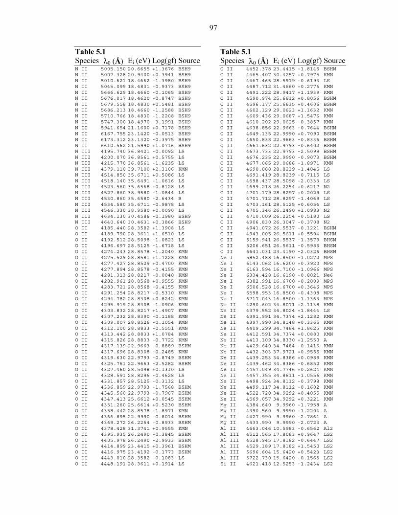
section 5.4.1. The wavelengths, gf values, and lower energy levels for the atomic
transitions used in the abundance analysis appear in Table 5.1.
The partition functions used to solve the Boltzmann equation were interpolated
directly from the partition functions used in ATLAS9 (Kurucz 1993). The weights of
atomic nuclei were taken from Coplen (1997), and the ionization energies for each
atomic species are from the Table of Ground Levels and Ionization Energies of Neutral
Atoms at the National Institute of Standards and Technology
(http://physics.nist.gov/PhysRefData/IonEnergy/ionEnergy.html) (Martin & Wiese
1996).
Table 5.1 Atomic Data For the Abundance Analysis Table 5.1 Species λ0=(Å) Ei (eV) Log(gf) SourceC II 4313.106 23.1161 -0.8590 LSC II 4318.606 23.1141 -0.9373 LSC II 4374.272 24.6535 +1.4605 KMNC II 4376.562 24.6600 +0.8136 KMNC II 4411.200 24.6019 +1.1909 KMNC II 4411.520 24.6033 +1.5476 KMNC II 4637.630 20.1500 -3.0857 BC II 5133.280 20.7040 -0.4835 AC II 5143.490 20.7040 -0.5665 AC II 5145.160 20.7100 +0.3612 AC II 5151.090 20.7100 -0.4904 AC II 6098.510 22.5710 +0.5206 LSC II 6578.050 14.4490 -0.0598 LSC II 6582.880 14.4490 -0.7529 LSC III 4186.900 40.0100 2.1137 N4C III 4325.560 38.4300 +0.2070 KMNC III 4515.811 39.4018 -0.6425 LSC III 4516.788 39.4024 -0.1335 LSC III 4647.418 29.5347 +0.1613 LSC III 4650.246 29.5347 -0.3477 LSC III 4659.058 38.2180 -1.5060 LSC III 4663.642 38.2180 -1.2204 LSC III 5695.920 32.1030 +0.0392 N2C III 5826.420 40.1970 +1.0845 N2N II 4227.750 21.5995 -0.1405 BSH9
Table 5.1 Species λ0=(Å) Ei (eV) Log(gf) SourceN II 4241.800 23.2463 +1.6864 KMNN II 4427.236 23.4220 -0.0101 KMNN II 4427.964 23.4220 -0.3798 KMNN II 4432.730 23.4156 +1.3297 KMNN II 4433.480 23.4255 -0.1054 KMNN II 4441.990 23.4220 +0.6831 KMNN II 4447.030 20.4091 +0.5247 BSH9N II 4507.560 20.6655 -1.8332 BSH9N II 4530.410 23.4748 +1.5454 KMNN II 4601.478 18.4662 -0.9854 BSH9N II 4607.153 18.4623 -1.1673 BSH9N II 4613.868 18.4662 -1.5311 BSH9N II 4621.393 18.4662 -1.1835 BSH9N II 4630.539 18.4832 +0.2167 BSH9N II 4643.086 18.4831 -0.8267 BSH9N II 4654.531 18.4969 -4.1624 BSH9N II 4674.908 18.4969 -4.2398 BSH9N II 4678.100 23.5721 +0.1823 KMNN II 4694.700 23.5721 +0.2546 KMNN II 4779.722 20.6461 -1.3517 BSH9N II 4788.138 20.6536 -0.8359 BSH9N II 4803.287 20.6655 -0.2602 BSH9N II 4810.299 20.6655 -2.4960 BSH9N II 4895.117 17.8770 -3.0850 BSH9N II 5002.703 18.4623 -2.3532 BSH9
97
Table 5.1 Species λ0=(Å) Ei (eV) Log(gf) SourceN II 5005.150 20.6655 +1.3676 BSH9N II 5007.328 20.9400 +0.3941 BSH9N II 5010.621 18.4662 -1.3980 BSH9N II 5045.099 18.4831 -0.9373 BSH9N II 5666.629 18.4660 -0.1065 BSH9N II 5676.017 18.4620 -0.8747 BSH9N II 5679.558 18.4830 +0.5481 BSH9N II 5686.213 18.4660 -1.2588 BSH9N II 5710.766 18.4830 -1.2208 BSH9N II 5747.300 18.4970 -3.1991 BSH9N II 5941.654 21.1600 +0.7178 BSH9N II 6167.755 23.1420 -0.0513 BSH9N II 6173.312 23.1320 -0.3975 BSH9N II 6610.562 21.5990 +1.0716 BSH9N III 4195.740 36.8421 -0.0092 LSN III 4200.070 36.8561 +0.5755 LSN III 4215.770 36.8561 -1.6235 LSN III 4379.110 39.7100 +2.3106 KMNN III 4514.850 35.6711 +0.5086 LSN III 4518.140 35.6491 -1.0616 LSN III 4523.560 35.6568 -0.8128 LSN III 4527.860 38.9580 -1.0844 LSN III 4530.860 35.6580 -2.6434 BN III 4534.580 35.6711 -0.9878 LSN III 4546.330 38.9580 +0.0090 LSN III 4634.130 30.4586 -0.1980 BSH9N III 4640.640 30.4631 +0.3866 BSH9O II 4185.440 28.3582 +1.3908 LSO II 4189.790 28.3611 +1.6510 LSO II 4192.512 28.5098 -1.0823 LSO II 4196.697 28.5125 -1.6718 LSO II 4274.243 28.8578 -1.2040 KMNO II 4275.529 28.8581 +1.7228 KMNO II 4277.427 28.8529 +0.4700 KMNO II 4277.894 28.8578 -0.4155 KMNO II 4281.313 28.8217 -0.0040 KMNO II 4282.961 28.8568 +0.9555 KMNO II 4283.721 28.8568 -0.4155 KMNO II 4291.254 28.8217 -0.5310 KMNO II 4294.782 28.8308 +0.8242 KMNO II 4295.919 28.8308 -1.0906 KMNO II 4303.832 28.8217 +1.4907 KMNO II 4307.232 28.8390 -0.1188 KMNO II 4309.007 28.8526 -0.1054 KMNO II 4312.100 28.8833 -0.5551 KMNO II 4313.442 28.8833 +1.0784 KMNO II 4315.826 28.8833 -0.7722 KMNO II 4317.139 22.9663 -0.8889 BSHMO II 4317.696 28.8308 -0.2485 KMNO II 4319.630 22.9793 -0.8749 BSHMO II 4325.761 22.9663 -2.5282 BSHMO II 4327.460 28.5098 +0.1310 LSO II 4328.591 28.8296 -0.4628 LSO II 4331.857 28.5125 -0.3132 LSO II 4336.859 22.9793 -1.7568 BSHMO II 4345.560 22.9793 -0.7967 BSHMO II 4347.413 25.6612 +0.0545 BSHMO II 4351.260 25.6614 +0.5230 BSHMO II 4358.442 28.8578 -1.8971 KMNO II 4366.895 22.9990 -0.8014 BSHMO II 4369.272 26.2254 -0.8933 BSHMO II 4378.428 31.3741 +0.9555 KMNO II 4395.935 26.2490 -0.3845 BSHMO II 4405.978 26.2490 -2.9933 BSHMO II 4414.899 23.4415 +0.3961 BSHMO II 4416.975 23.4192 -0.1773 BSHMO II 4443.010 28.3582 -0.1083 LSO II 4448.191 28.3611 +0.1914 LS
Table 5.1 Species λ0=(Å) Ei (eV) Log(gf) SourceO II 4452.378 23.4415 -1.8146 BSHMO II 4465.407 30.4257 +0.7975 KMNO II 4467.465 28.5919 -0.6193 LSO II 4487.712 31.4660 +0.2776 KMNO II 4491.222 28.9417 +1.1939 KMNO II 4590.974 25.6612 +0.8056 BSHMO II 4596.177 25.6635 +0.4606 BSHMO II 4602.129 29.0623 +1.1632 KMNO II 4609.436 29.0687 +1.5476 KMNO II 4610.202 29.0625 -0.3857 KMNO II 4638.856 22.9663 -0.7644 BSHMO II 4649.135 22.9990 +0.7090 BSHMO II 4650.838 22.9663 -0.8336 BSHMO II 4661.632 22.9793 -0.6402 BSHMO II 4673.733 22.9793 -2.5099 BSHMO II 4676.235 22.9990 -0.9073 BSHMO II 4677.065 29.0686 -1.8971 KMNO II 4690.888 28.8239 -1.4045 LSO II 4691.419 28.8239 -0.7115 LSO II 4698.437 28.5098 -2.0333 LSO II 4699.218 26.2254 +0.6217 N2O II 4701.179 28.8297 +0.2029 LSO II 4701.712 28.8297 -1.4069 LSO II 4703.161 28.5125 +0.6054 LSO II 4705.346 26.2490 +1.0983 N2O II 4710.009 26.2254 -0.5180 LSO II 4906.830 26.3047 -0.3708 N2O II 4941.072 26.5537 -0.1221 BSHMO II 4943.005 26.5611 +0.5504 BSHMO II 5159.941 26.5537 -1.3579 BHSMO II 5206.651 26.5611 -0.5986 BHSMO II 6641.031 23.4190 -2.0326 BHSMNe I 5852.488 16.8500 -1.0272 MPSNe I 6143.062 16.6200 +0.3920 MPSNe I 6163.594 16.7100 -1.0966 MPSNe I 6334.428 16.6190 -0.8021 Ne6Ne I 6382.991 16.6700 -0.2009 MPSNe I 6506.528 16.6700 +0.3646 MPSNe I 6598.953 16.8500 -0.4308 MPSNe I 6717.043 16.8500 -1.1363 MPSNe II 4290.602 34.8071 +2.1138 KMNNe II 4379.552 34.8024 +1.8444 LSNe II 4391.991 34.7374 +2.1282 KMNNe II 4397.990 34.8148 +0.3365 KMNNe II 4409.299 34.7484 +1.8625 KMNNe II 4412.591 34.7374 +0.0880 KMNNe II 4413.109 34.8330 +1.2550 ANe II 4429.640 34.7484 -0.1416 KMNNe II 4432.303 37.9721 +0.9555 KMNNe II 4439.253 34.8386 +0.0989 KMNNe II 4439.462 34.8386 -0.6852 KMNNe II 4457.049 34.7746 +0.2624 KMNNe II 4457.355 34.8611 -1.0556 KMNNe II 4498.924 34.8112 -0.3798 KMNNe II 4499.117 34.8112 -0.1602 KMNNe II 4522.720 34.9292 +0.4055 KMNNe II 4569.057 34.9292 +0.3221 KMNMg II 4384.640 9.9960 -1.7958 AMg II 4390.560 9.9990 -1.2204 AMg II 4427.990 9.9960 -2.7861 AMg II 4433.990 9.9990 -2.0723 AAl II 4663.046 10.5983 -0.6562 Al2Al III 4512.565 17.8083 +0.9647 LS2Al III 4528.945 17.8182 -0.6447 LS2Al III 4529.189 17.8182 +1.5450 LS2Al III 5696.604 15.6420 +0.5423 LS2Al III 5722.730 15.6420 -0.1565 LS2Si II 4621.418 12.5253 -1.2434 LS2

98
Table 5.1 Species λ0=(Å) Ei (eV) Log(gf) SourceSi II 4621.722 12.5255 -0.8911 LS2Si II 5041.024 10.0664 +0.4008 LS2Si II 5055.984 10.0739 +1.0156 LS2Si II 5957.560 10.0660 -0.8052 SiBSi II 5978.930 10.0740 -0.1416 SiBSi II 6371.355 8.1200 -0.1154 SiASi III 4552.622 19.0163 +0.6724 LS2Si III 4553.997 28.1224 -0.3431 LS2Si III 4567.840 19.0163 +0.1613 LS2Si III 4574.757 19.0163 -0.9350 LS2Si III 4683.020 28.1224 +0.4253 KMNSi III 4716.654 25.3338 +1.8789 LS2Si III 4813.330 25.9788 +1.6174 KMNSi III 4828.960 25.9873 +2.1282 KMNSi III 5114.116 28.5500 +0.6445 SiB
Si III 5739.730 19.7220 -0.3615 SiBSi IV 4314.102 34.2821 -0.5065 LS2Si IV 4631.240 36.4169 +2.7344 KMNSi IV 4654.320 36.4316 +3.4210 KMNSi IV 6667.570 34.2820 +1.1122 LS2P III 4246.680 14.6100 -0.2533 AS II 4259.146 17.4457 +1.1836 LS2S II 4267.762 16.1004 +0.6770 LS2S II 4269.760 16.0920 -0.2758 LS2S II 4278.540 16.0920 -0.2758 LS2S II 4282.630 16.1000 -0.0233 LS2S II 4291.450 16.1000 -1.8643 LS2S II 4294.402 16.1346 +1.3239 LS2S II 4432.410 15.8670 -1.0593 LS2S II 4456.430 15.8480 -1.2895 LS2S II 4463.580 15.9440 -0.0460 LS2S II 4483.420 15.8990 -0.9902 LS2S II 4486.660 15.8670 -0.9211 LS2S II 4524.680 15.0680 -2.1646 LS2S II 4524.950 15.0680 +0.1840 LS2S II 4552.380 15.0680 -0.2303 LS2S II 4656.740 13.5840 -1.8650 LS2S II 4716.230 13.6170 -1.1973 LS2S II 4792.020 16.1350 -0.2763 LS2S II 4815.520 13.6720 -0.1151 LS2S II 4824.070 16.2650 +0.0459 LS2S II 4835.850 16.1000 -2.2798 LS2S II 4885.630 14.0030 -1.7037 LS2S II 4917.150 14.0030 -0.9211 LS2S II 4925.320 13.5840 -1.0823 LS2S II 4942.470 13.5840 -2.2109 LS2S II 4991.940 13.6170 -1.4966 LS2S II 5009.540 13.6170 -0.6447 LS2S II 5014.030 14.0680 +0.0695 LS2S II 5027.190 13.0930 -1.6581 LS2S II 5032.410 13.6720 +0.4148 LS2S II 5103.300 13.6720 -0.2533 LS2S II 5142.330 13.1480 -1.9112 LS2S II 5606.151 13.7330 +0.7129 LS2S II 5616.633 13.6600 -1.4828 LS2S II 5647.020 14.0020 +0.0862 LS2S II 5660.001 13.6770 -0.1222 LS2S II 5664.773 13.6600 -0.5825 LS2S II 5819.254 14.0670 -1.7568 LS2S III 4253.499 18.2439 +0.8242 LS2S III 4284.990 18.1931 +0.2143 LS2S III 4332.653 18.1882 -0.6149 LS2S III 4361.468 18.2439 -0.9188 LS2S III 4364.661 18.3181 -1.6394 LS2S III 4439.870 18.2940 -3.7533 LS2S III 4467.716 18.3115 -2.2266 LS2Ar II 4228.158 16.7488 -1.5422 Ar1Ar II 4331.199 16.7485 -0.4374 Ar1
Table 5.1 Species λ0=(Å) Ei (eV) Log(gf) SourceAr II 4370.753 18.6568 -0.2796 Ar1Ar II 4371.329 16.4258 -1.3736 Ar1Ar II 4400.986 16.4065 -0.6354 Ar1Ar II 4426.001 16.7485 +0.3660 Ar1Ar II 4430.189 16.8125 -0.4006 Ar1Ar II 4448.879 21.4981 +0.1467 Ar2Ar II 4545.052 17.1400 -0.5389 Ar1Ar II 4579.349 17.2658 -0.6862 Ar1Ar II 4589.898 18.4266 +0.2303 Ar1Ar II 4735.905 16.6439 -0.2487 Ar1Ar II 4806.020 16.6439 +0.4837 Ar1Ar II 4847.809 16.7485 -0.5135 Ar1Ar II 4879.863 17.1400 +0.5664 Ar1Sc II 4246.822 0.3150 +0.0450 LS3Sc II 4314.083 0.6184 -0.7818 LS3Sc II 4320.732 0.6055 -1.0909 LS3Sc II 4324.996 0.5955 -1.4221 LS3Sc II 4374.457 0.6184 -1.5498 LS3Sc II 4400.389 0.6055 -1.7958 LS3Sc II 4670.407 1.3570 -1.8859 LS3Ti II 4171.920 2.5977 -1.2895 KTi II 4174.050 2.5977 -2.8783 KTi II 4184.303 1.0800 -5.7796 Bz93Ti II 4287.880 1.0799 -4.6512 KTi II 4290.220 1.1650 -2.5789 KTi II 4294.090 1.0841 -2.5559 KTi II 4300.049 1.1801 -1.1282 Bz93Ti II 4301.920 1.1610 -2.6710 KTi II 4307.863 1.1649 -2.5329 Bz93Ti II 4312.870 1.1801 -2.6710 KTi II 4314.970 1.1610 -2.6019 KTi II 4316.800 2.0477 -3.2696 KTi II 4320.960 1.1650 -4.3058 KTi II 4337.880 1.0799 -2.6019 KTi II 4350.850 2.0613 -3.2236 KTi II 4367.650 2.5903 -2.9243 KTi II 4391.040 1.2313 -6.3323 KTi II 4394.051 1.2214 -4.0757 Bz93Ti II 4395.850 1.2429 -4.5356 Bz93Ti II 4399.790 1.2369 -2.9243 KTi II 4407.680 1.2214 -5.6875 KTi II 4409.220 1.2430 -5.1809 KTi II 4411.100 3.0948 -2.4407 KTi II 4417.720 1.1650 -3.2928 KTi II 4418.330 1.2369 -4.5824 Bz93Ti II 4421.950 2.0613 -4.0757 KTi II 4441.730 1.1801 -5.5493 KTi II 4443.794 1.0800 -1.6119 Bz93Ti II 4444.558 1.1156 -5.0887 Bz93Ti II 4450.482 1.0842 -3.4770 Bz93Ti II 4464.460 1.1610 -4.7893 KTi II 4468.507 1.1305 -1.3815 Bz93Ti II 4488.340 3.1236 -1.8878 KTi II 4501.273 1.1156 -1.7499 Bz93Ti II 4529.480 1.5718 -4.6742 KTi II 4533.970 1.2369 -1.7731 KTi II 4549.610 1.5839 -1.0362 KTi II 4563.770 1.2214 -2.2109 KTi II 4571.960 1.5718 -1.2204 KCr II 4539.610 4.0424 -5.8256 KCr II 4555.010 4.0713 -3.1775 KCr II 4558.660 4.0734 -1.5196 KCr II 4565.770 4.0424 -4.8585 KCr II 4588.220 4.0713 -1.4507 KCr II 4592.070 4.0735 -2.8091 KCr II 4616.640 4.0723 -2.9703 KCr II 4618.820 4.0735 -2.5559 KCr II 4634.100 4.0723 -2.8553 K

99
Table 5.1 Species λ0=(Å) Ei (eV) Log(gf) SourceCr II 4876.410 3.8645 -3.3619 N9Fe I 4175.640 2.8451 -1.5427 LS4Fe I 4181.750 2.8316 -0.4145 LS4Fe I 4184.890 2.8316 -1.9805 LS4Fe I 4187.040 2.4496 -1.2620 LS4Fe I 4187.790 2.4254 -1.2755 LS4Fe I 4202.030 1.4848 -1.6302 LS4Fe I 4233.600 2.4822 -1.3907 LS4Fe I 4235.940 2.4254 -0.7853 LS4Fe I 4238.810 3.3965 -0.6287 LS4Fe I 4247.430 3.3683 -0.5297 LS4Fe I 4250.120 2.4688 -0.9324 LS4Fe I 4250.790 1.5574 -1.6348 LS4Fe I 4260.473 2.3992 -0.0414 LS4Fe I 4271.150 2.4496 -0.8036 LS4Fe I 4271.760 1.4848 -0.3776 LS4Fe I 4282.400 2.1759 -1.8650 LS4Fe I 4325.760 1.6080 -0.0231 LS4Fe I 4369.770 3.0469 -1.6809 LS4Fe I 4383.540 1.4848 +0.4606 LS4Fe I 4404.750 1.5574 -0.3270 LS4Fe I 4415.120 1.6080 -1.4159 LS4Fe I 4466.550 2.8316 -1.3587 LS4Fe I 4494.560 2.1979 -2.6158 LS4Fe I 4528.610 2.1759 -1.8925 LS4Fe II 4173.450 2.5827 -5.0196 LS4Fe II 4178.860 2.5827 -5.7105 LS4Fe II 4233.170 2.5827 -4.6052 LS4Fe II 4258.160 2.7044 -7.8288 LS4Fe II 4273.320 2.7044 -7.6906 LS4Fe II 4296.570 2.7044 -6.9308 LS4Fe II 4303.170 2.7044 -5.7334 LS4Fe II 4351.760 2.7044 -4.8355 LS4Fe II 4369.400 2.7785 -8.4505 LS4Fe II 4384.330 2.6570 -8.0591 LS4
Table 5.1 Species λ0=(Å) Ei (eV) Log(gf) SourceFe II 4413.600 2.6759 -8.9110 LS4Fe II 4416.820 2.7785 -5.9867 LS4Fe II 4472.920 2.8441 -7.8980 LS4Fe II 4489.190 2.8281 -6.8382 LS4Fe II 4491.400 2.8555 -6.2171 LS4Fe II 4508.280 2.8555 -5.0887 LS4Fe II 4515.340 2.8441 -5.7105 LS4Fe II 4520.230 2.8067 -5.9867 LS4Fe II 4522.630 2.8441 -4.6742 LS4Fe II 4541.520 2.8555 -7.0228 LS4Fe II 4549.210 5.9110 -4.3058 LS4Fe II 4549.470 2.8281 -4.0297 LS4Fe II 4555.890 2.8281 -5.2728 LS4Fe II 4576.330 2.8441 -6.9999 LS4Fe II 4582.840 2.8441 -7.1380 LS4Fe II 4583.830 2.8067 -4.6512 LS4Fe II 4620.510 2.8281 -7.5525 LS4Fe II 4629.340 2.8067 -5.4571 LS4Fe II 4635.330 5.9561 -3.7991 LS4Fe II 4656.970 2.8911 -8.3585 LS4Fe II 4666.750 2.8281 -7.6677 LS4Fe II 4670.170 2.5827 -9.4406 LS4Fe II 4731.440 2.8911 -7.7367 LS4Fe II 5197.560 3.2304 -4.8355 LS4Fe II 5961.710 10.6780 +1.5892 LS4Fe III 4222.271 20.8704 +0.5878 KMNFe III 4296.851 22.8598 +2.1199 KMNFe III 4310.355 22.8688 +2.7206 KMNFe III 4372.536 22.9100 +2.2460 KMNFe III 4372.823 22.9101 +2.5611 KMNY II 4177.536 0.4080 -0.3708 YY II 4309.622 0.1790 -1.7198 YY II 4422.588 0.1030 -2.9243 YBa II 4554.036 0.0000 +0.2761 G67
Sources for Table 5.1: A Wiese, Smith, & Glennon(1966) Al2 Zare(1967) Ar1 Bennett(1965) Ar2 Rudko & Tang(1968) B Kurucz & Peytreman (1975) BSH9 Bell et al.(1995) BSHM Bell et al.(1994) Bz93 Bizzarri et al.(1993) G67 Gallagher (1967) K Savanov, Huovelin, & Tuominen(1990) KMN Kilian, Montenbruck, & Nissen(1991) LS Wiese et al.(1996)
LS2 Wiese, Smith, & Miles(1969) LS3 Martin, Furh, & Wiese(1988) LS4 Fuhr, Martin, & Wiese(1988) MPS Magazzu et al.(1981) N2 Yu Yan & Seaton(1987) N4 Nussbaumer & Storey(1981) N9 Kostyk & Orlova(1983) Ne6 Krebs(1936) SiA Lambert & Luck(1978) SiB Lambert & Warner(1968) Y Hannaford et al.(1982)

100
5.3 Microturbulence
Equivalent widths are affected by microturbulence through the damping
constant. Microturbulence plays a large role in LTE analysis of stars, particularly in the
atmospheres of super-giants which have microturbulence values that approach or
exceed the thermal velocities of hydrogen and helium in their stellar atmospheres
(Villamariz & Herrero 2000). The physical explanation for large microturbulent
velocities in B stars is uncertain but it may be a product of a wind driven outflow that
sets up a velocity gradient in the photosphere producing a slope in the curve of growth
that mimics the effect of microturbulence (Kudritski 1992; Lamers & Achmad 1994}.
The microturbulent velocity (ξt) is determined by finding the value at which the
slope of abundance versus equivalent width is zero for the lines of a given atomic
species. Species with many lines that span a large range of equivalent widths are the
best barometers of microturbulence. For hotter B Stars, O II, N II, and Si III have well
populated curves of growth that are ideal for determining the microturbulence. For
cooler B stars, Fe II, Cr II, and Ti II are good species to use. Theoretically, the
microturbulent velocity should be the same for all species. However in practice, there is
sometimes a discrepancy between the results measured from different elements and
ionization stages. Of particular note, in early type B supergiants Si III sometimes
indicates a smaller microturbulence than O II (McErlean, Lennon, & Dufton 1998;
Vrancken 1998). McErlean, Lennon, & Dufton (1999) suggest that in these
circumstance the Si III 4550 Å triplet gives a better answer since the lines in the triplet
cover a range of strengths and are from the same multiplet, thus less susceptible to
systematic errors in the atomic data.

101
For this study the microturbulent velocity obtained by balancing the Si III 4450
Å triplet has been given preference. When the Si III 4550 Å triplet is not available, a
consensus between the other species with the best populated curves of growth was used.
In the cases where fewer than three lines of any species were measured, making it
impossible to determine the microturbulent velocity, the value used is “borrowed” from
another star with a similar effective temperature and gravity. The microturbulent
velocities assigned to each star are listed in Table 5.2.
The LTE microturbulence values for B stars are typically on the order of 5 km/s
to 10 km/s or more. Microturbulent velocities of this magnitude dominate the damping
parameter for most elements since at 20000 K the thermal velocities of hydrogen and
iron atoms are 12.8 km/s and 1.7 km/s respectively. NLTE analysis of the same stars
normally uses smaller microturbulent velocities (1 km/s to 5 km/s). This apparent
correlation has led to speculation, but few conclusions, about the connection of
microturbulence and NLTE effects. The relationship between NLTE effects and
microturbulence will be discussed in more detail in Section 5.6.1.
5.4 Abundances From Equivalent Widths
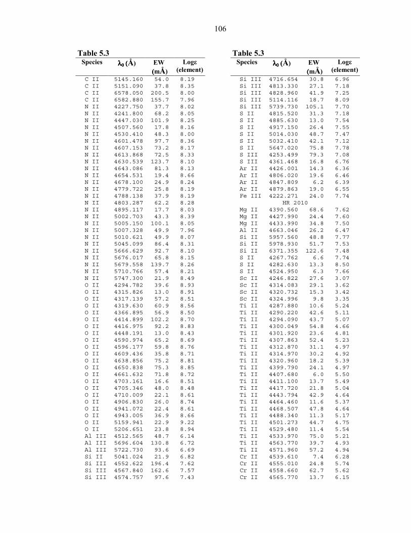
The measured equivalent widths and absolute abundances derived for individual
lines are listed in Table 5.3 and the average absolute abundances for each star are in
Tables 5.4 through 5.6. The abundances given for the eclipsing binary HIP 76161 (IT
Lib) are from the primary component. The procedure used to correct the equivalent
widths of HIP 76161A for the continuum contribution from the secondary component is
outlined in Martin (2003).

102
Table 5.2 Microturbulent Velocities for Sample Stars
Star
Teff (K)
Log(g) (dex)
ξt (km/s)
Determined From
Nearby Pop I Control SampleGam Peg 21750 3.75 7 Si III, O IIHR 1220 28750 3.75 19 Si III, O II, N IIHR 1397 14250 4.00 0.1 Fe II, S IIBet Ori 18000 3.50 7 Si III, N II, Fe IIGam Ori 21750 4.00 8.7 Si III, O IIHR 2010 10750 4.25 3 Fe IIHR 2928 23750 4.00 7.6 Si IIIHR 4187 10250 4.25 3.8 Fe II, Ti IIHR 6165 30000 3.75 7 Si III, O II, N IINu Cap 10250 4.25 2.5 Fe II, Ti IIHR 8404 10250 3.50 0.5 Fe IIHR 8768 17750 3.75 8 Si III
BHB Control SampleHD 60778 8750 3.25 5 Fe II, Ti IIHD 74721 8750 3.50 2.25 Fe II, Ti II
PAGB Control SampleHD 18100 27000 4.25 10 borrowedHD 44179 8250 2.50 2 borrowedHD 105262 9000 2.50 2 Fe IIHD 119608 26500 4.00 15 Si III, N II
Sample of StudyHIP 1214 11500 4.00 10 Fe IIHIP 1511 9000 3.00 2 Fe II, Cr IIHIP 3013 19750 4.00 8 Si IIIHIP 6727 10000 3.00 2 Fe II, Cr II, Ti IIHIP 11809 13250 4.25 5 borrowedHIP 11844 11250 4.00 5 Fe IIHIP 12320 13500 4.00 5 borrowedHIP 15967 18500 4.00 9 Si IIIHIP 16130 13500 4.25 5 Fe IIHIP 28132 17000 3.50 6 Si III, O II, N IIHIP 37903 18000 3.00 17 Si III, O II, N IIHIP 41979 18000 4.50 10 Si IIIHIP 45904 21250 3.50 15 Si IIIHIP 48394 20250 3.75 10 borrowedHIP 52906 18500 3.75 10 Si IIIHIP 55416 15500 4.50 5 borrowedHIP 56322 26000 4.25 10 borrowedHIP 58046 13250 4.50 5 borrowedHIP 59067 15000 3.75 5 borrowedHIP 59955 13500 4.50 5 borrowedHIP 60615 22000 3.75 7 N IIHIP 61800 12500 3.25 1 N II, Fe IIHIP 63591 10000 3.25 5 borrowedHIP 65388 20000 4.75 6 Si III, N II, O IIHIP 66291 17500 4.25 5 Si IIIHIP 69247 11250 2.50 3 Fe IIHIP 75577 12250 2.75 5 S IIHIP 76161 22000 4.00 12 Si IIIHIP 77131 32000 3.75 15 Si IIIHIP 77716 21500 3.25 7 Si IIIHIP 79649 21000 3.75 10 Si III, O IIHIP 81153 30000 4.00 20 Si III, O IIHIP 96130 23000 3.50 15 Si IIIHIP 98136 23250 3.50 15 Si IIIHIP 107027 22000 3.50 10 Si III, O IIHIP 109051 21000 4.25 10 Si III, O IIHIP 111396 13750 3.75 5 Fe IIHIP 112790 15250 4.00 5 borrowedHIP 114569 17750 4.25 5 Si IIIHIP 115729 17750 4.00 10.0 Si IIIHIP 116560 8250 3.25 0.5 Fe I

103
Table 5.3 Equivalent Widths and Abundances for Single Lines Table 5.3
Species λλλλ0000====((((Å) EW=
==
==
==
=
((((mÅ) Logε
(element)Nearby Pop I Control Sample
Gam PegC II 4313.106 9.6 8.31C II 4318.606 8.3 8.27C II 4374.272 25.8 8.12C II 4376.562 7.6 7.88C II 4411.200 21.8 8.17C II 4411.520 23.9 8.05N II 4227.750 17.5 7.54N II 4241.800 32.8 7.52N II 4427.236 10.5 7.72N II 4432.730 17.5 7.40N II 4433.480 7.6 7.61N II 4441.990 11.4 7.46N II 4447.030 40.6 7.46N II 4507.560 8.0 7.70N II 4530.410 21.6 7.45N II 4601.478 38.0 7.59N II 4607.153 33.9 7.60O II 4189.790 41.3 8.38O II 4192.512 5.6 8.40O II 4196.697 4.6 8.56O II 4274.243 4.1 8.41O II 4275.529 23.0 8.07O II 4277.427 13.8 8.30O II 4277.894 10.9 8.55O II 4281.313 4.8 7.95O II 4282.961 12.4 8.03O II 4283.721 8.6 8.43O II 4291.254 15.9 8.80O II 4294.782 23.2 8.45O II 4295.919 2.5 8.12O II 4303.832 31.8 8.39O II 4307.232 15.7 8.63O II 4309.007 10.6 8.41O II 4312.100 8.7 8.51O II 4313.442 11.1 7.93O II 4317.139 61.0 8.50O II 4317.696 6.4 8.21O II 4319.630 54.5 8.40O II 4325.761 21.0 8.43O II 4327.460 9.9 8.19O II 4328.591 6.2 8.28O II 4331.857 6.9 8.21O II 4336.859 11.6 7.78O II 4345.560 28.6 7.88O II 4347.413 21.5 7.99O II 4351.260 38.1 8.14O II 4358.442 4.9 8.82O II 4366.895 52.4 8.35O II 4369.272 16.5 8.39O II 4378.428 9.2 8.47O II 4414.899 75.1 8.31O II 4416.975 65.8 8.42
Table 5.3 Species λλλλ0000====((((Å) EW=
==
==
==
=
((((mÅ) Logε
(element)O II 4443.010 11.1 8.37O II 4448.191 13.5 8.34O II 4452.378 30.5 8.51O II 4465.407 12.8 8.53O II 4487.712 3.9 8.41O II 4491.222 17.5 8.21O II 4590.974 52.4 8.41O II 4596.177 51.8 8.55O II 4602.129 11.6 8.05O II 4609.436 29.7 8.47Ne II 4409.299 4.8 8.16Mg II 4384.640 10.2 7.60Mg II 4390.560 14.1 7.51Mg II 4433.990 5.9 7.47Al III 4512.565 37.5 5.94Al III 4529.189 56.9 5.97Si III 4552.622 131.8 7.11Si III 4553.997 5.0 7.51Si III 4567.840 105.1 7.03Si III 4574.757 71.2 7.09P III 4246.680 10.1 5.03S II 4269.760 5.9 7.16S II 4278.540 2.8 6.83S II 4282.630 4.2 6.90S II 4294.402 15.0 6.91S II 4463.580 9.9 7.27S II 4483.420 4.3 7.28S II 4486.660 5.1 7.32S II 4524.680 2.9 7.39S II 4524.950 12.9 7.05S III 4253.499 40.7 6.43S III 4284.990 26.3 6.39S III 4361.468 17.4 6.66S III 4364.661 9.8 6.68S III 4439.870 10.2 7.46Ar II 4228.158 3.1 6.48Ar II 4331.199 11.5 6.60Ar II 4370.753 3.9 6.56�Ar II 4371.329 12.5 6.96Ar II 4426.001 17.0 6.45Ar II 4430.189 7.0 6.38Ar II 4448.879 4.6 7.21Ar II 4545.052 10.0 6.70Ar II 4579.349 6.7 6.62Ar II 4589.898 7.7 6.60Fe III 4222.271 23.1 7.64Fe III 4296.851 12.0 7.13Fe III 4310.355 16.0 7.02Fe III 4372.823 13.7 7.04
HR 1220N II 4227.750 38.8 8.23N II 4241.800 110.5 8.35N II 4427.236 66.9 8.83N II 4432.730 69.6 8.27

104
Table 5.3 Species λλλλ0000====((((Å) EW=
==
==
==
=
((((mÅ) Logε
(element)N II 4441.990 135.2 8.97N II 4447.030 213.1 8.79N II 4601.478 136.5 8.69N II 4613.868 53.9 8.38N II 4630.539 153.2 8.25N III 4379.110 73.8 8.39O II 4185.440 83.8 8.44O II 4189.790 89.4 8.36O II 4303.832 97.3 8.59O II 4325.761 78.0 9.01O II 4366.895 136.8 8.63O II 4378.428 58.3 9.02O II 4395.935 57.9 8.59O II 4452.378 54.1 8.61O II 4590.974 167.9 8.65O II 4596.177 146.2 8.69O II 4661.632 232.8 9.02Al III 4529.189 149.0 6.93Si III 4552.622 302.6 7.54Si III 4567.840 251.1 7.54Si III 4574.757 163.8 7.64S II 4291.450 24.4 10.08S III 4253.499 194.7 7.08S III 4284.990 189.3 7.31Fe III 4372.536 61.2 8.02
HR 1397C II 4318.606 3.7 8.99C II 6578.050 59.8 8.60C II 6582.880 44.8 8.60N II 4432.730 5.0 8.63N II 4621.393 6.3 8.37N II 4630.539 5.7 7.71N II 4643.086 11.2 8.59Ne I 5852.488 24.2 8.62Ne I 6143.062 38.1 8.37Ne I 6163.594 10.5 8.11Ne I 6334.428 22.7 8.47Ne I 6382.991 24.0 8.29Ne I 6506.528 29.5 8.24Ne I 6598.953 19.1 8.33Ne I 6717.043 25.5 8.88Mg II 4384.640 15.4 7.18Mg II 4390.560 32.6 7.39Mg II 4427.990 7.4 7.24Mg II 4433.990 14.2 7.33Al II 4663.046 18.4 6.00Al III 4529.189 9.6 6.53Si II 4621.418 11.0 7.39Si II 4621.722 9.8 7.18Si II 5957.560 52.5 7.53Si II 5978.930 57.2 7.34Si II 6371.355 121.8 7.57S II 4267.762 11.6 7.10�S II 4269.760 8.1 7.29S II 4278.540 7.4 7.24S II 4282.630 9.1 7.25S II 4294.402 15.0 7.01S II 4432.410 4.9 7.33S II 4463.580 10.2 7.33
Table 5.3 Species λλλλ0000====((((Å) EW=
==
==
==
=
((((mÅ) Logε
(element)S II 4483.420 6.5 7.47S II 4486.660 4.9 7.28S II 4524.680 4.2 7.48S II 4524.950 11.9 7.04S II 4656.740 6.4 7.07S II 5606.151 17.7 6.89S II 5647.020 22.8 7.47S II 5660.001 12.9 7.01Ar II 4400.986 2.7 6.71Ar II 4426.001 4.5 6.69Ti II 4300.049 3.8 4.65Ti II 4464.460 5.5 6.40Cr II 4558.660 9.7 5.43Cr II 4588.220 7.6 5.27Fe II 4233.170 28.8 6.93Fe II 4258.160 3.2 7.17Fe II 4296.570 8.6 7.25Fe II 4303.170 13.7 6.98Fe II 4351.760 17.1 6.73Fe II 4416.820 15.2 7.18Fe II 4489.190 10.9 7.39Fe II 4491.400 10.2 7.10Fe II 4508.280 17.4 6.91Fe II 4515.340 14.2 7.05Fe II 4520.230 10.1 6.97Fe II 4522.630 23.4 6.92Fe II 4541.520 6.2 7.20Fe II 4549.470 40.4 7.12Fe II 4555.890 15.7 6.92Fe II 4576.330 8.0 7.31Fe II 4583.830 33.1 7.17Fe II 4629.340 12.9 6.88Fe II 4635.330 9.4 7.31
Bet OriC II 4637.630 7.0 8.54C II 5133.280 10.7 7.89C II 5145.160 21.1 7.88C II 5151.090 6.1 7.62C II 6578.050 228.8 8.67C II 6582.880 169.2 8.45N II 4227.750 10.7 7.63N II 4241.800 24.0 7.78N II 4432.730 8.5 7.44N II 4447.030 21.5 7.48N II 4530.410 7.3 7.32N II 4601.478 23.8 7.69N II 4607.153 19.3 7.65N II 4613.868 15.1 7.66N II 4621.393 15.9 7.54N II 4630.539 46.5 7.67N II 4643.086 28.3 7.75N II 4654.531 4.8 8.24N II 4779.722 8.4 7.95N II 4788.138 7.6 7.67N II 4803.287 10.6 7.60N II 4810.299 3.6 8.04N II 4895.117 10.0 8.03N II 5005.150 29.2 7.59N II 5010.621 18.8 7.85

105
Table 5.3 Species λλλλ0000====((((Å) EW=
==
==
==
=
((((mÅ) Logε
(element)N II 5045.099 23.6 7.81N II 5666.629 22.9 7.59N II 5676.017 15.4 7.68N II 5679.558 51.7 7.91N II 5686.213 14.8 7.83N II 5710.766 20.7 8.03O II 4275.529 4.5 7.83O II 4282.961 9.2 8.58O II 4294.782 28.2 9.45O II 4319.630 8.2 7.78O II 4325.761 13.3 8.77O II 4395.935 22.2 9.14O II 4414.899 11.6 7.59O II 4416.975 47.7 8.91O II 4491.222 24.4 9.32O II 4590.974 4.3 7.53O II 4596.177 17.3 8.52O II 4609.436 3.2 7.94O II 4638.856 9.8 7.96O II 4649.135 15.7 7.63O II 4650.838 5.2 7.64O II 4661.632 6.3 7.66O II 4676.235 7.2 7.87O II 4701.179 6.1 8.86O II 4703.161 7.8 8.77Ne I 5852.488 23.2 8.40Ne I 6143.062 65.6 8.37Ne I 6163.594 14.3 8.17Ne I 6334.428 46.6 8.68Ne I 6382.991 33.1 8.23Ne I 6506.528 25.9 7.86Ne I 6598.953 21.8 8.19Ne I 6717.043 24.4 8.57Ne II 4290.602 4.3 9.05Mg II 4384.640 20.5 7.64Mg II 4390.560 21.3 7.41Al II 4663.046 28.5 6.65Al III 4512.565 13.5 5.65Al III 4529.189 30.2 5.88Al III 5696.604 51.7 6.34Al III 5722.730 32.2 6.30Si II 5041.024 139.4 7.79Si II 5055.984 215.5 8.25Si II 5978.930 108.5 7.83Si II 6371.355 486.4 9.46Si III 4552.622 65.9 6.96Si III 4567.840 44.0 6.80Si III 4574.757 21.2 6.73Si III 4716.654 32.7 7.70Si III 4828.960 5.9 6.69Si III 5739.730 26.9 7.25S II 4269.760 5.6 6.78S II 4278.540 8.4 6.96S II 4282.630 8.5 6.86S II 4291.450 5.4 7.45S II 4294.402 29.5 6.89S II 4456.430 5.1 7.12S II 4463.580 10.0 6.91S II 4524.950 20.7 6.89
Table 5.3 Species λλλλ0000====((((Å) EW=
==
==
==
=
((((mÅ) Logε
(element)S II 4656.740 11.1 7.00S II 4716.230 35.3 7.30S II 4792.020 7.4 6.97S II 4815.520 70.2 7.29S II 4824.070 18.2 7.30S II 4835.850 4.8 7.63S II 4885.630 19.3 7.35S II 4917.150 33.5 7.30S II 4925.320 58.5 7.56S II 4942.470 11.8 7.20S II 4991.940 27.5 7.32�S II 5009.540 43.4 7.20S II 5014.030 71.3 7.37S II 5027.190 27.9 7.23S II 5032.410 88.8 7.27S II 5103.300 28.1 6.80S II 5142.330 19.9 7.19S II 5606.151 66.8 6.99S II 5616.633 14.7 7.06S II 5647.020 61.5 7.30S II 5660.001 49.7 7.14S II 5664.773 33.5 7.10S II 5819.254 18.5 7.45S III 4253.499 7.0 5.93S III 4361.468 13.7 7.12Ar II 4228.158 5.5 6.67Ar II 4426.001 7.6 6.03Ar II 4579.349 6.4 6.58Ar II 4735.905 6.8 6.26Ar II 4806.020 7.3 5.99Ar II 4847.809 15.2 6.82Ar II 4879.863 6.8 6.08Fe II 4233.170 125.1 8.78Fe II 4273.320 11.4 8.71Fe II 4296.570 19.4 8.63Fe II 4303.170 46.4 8.57Fe II 4351.760 79.4 8.52Fe II 4489.190 14.9 8.51Fe II 4491.400 26.1 8.53Fe II 4508.280 59.6 8.49Fe II 4515.340 39.6 8.52Fe II 4520.230 38.5 8.61Fe II 4541.520 18.2 8.70Fe II 4549.470 126.5 8.63Fe II 4555.890 50.6 8.46Fe II 4576.330 16.0 8.62Fe II 4583.830 120.2 8.84Fe II 4620.510 8.9 8.59Fe II 4629.340 44.4 8.46Fe II 4635.330 22.2 8.46Fe II 4666.750 9.6 8.67Fe II 4731.440 10.3 8.76Fe II 5197.560 38.3 8.27Fe III 4222.271 4.2 7.17Fe III 4296.851 20.7 7.97
Gam OriC II 4411.200 27.6 8.29C II 5133.280 67.8 8.71C II 5143.490 28.2 8.22
106
Table 5.3 Species λλλλ0000====((((Å) EW=
==
==
==
=
((((mÅ) Logε
(element)C II 5145.160 54.0 8.19C II 5151.090 37.8 8.35C II 6578.050 200.5 8.00C II 6582.880 155.7 7.96N II 4227.750 37.7 8.02N II 4241.800 68.2 8.05N II 4447.030 101.9 8.25N II 4507.560 17.8 8.16N II 4530.410 48.3 8.00N II 4601.478 97.7 8.36N II 4607.153 73.2 8.17N II 4613.868 72.5 8.33N II 4630.539 123.7 8.10N II 4643.086 81.3 8.13N II 4654.531 19.4 8.66N II 4678.100 24.9 8.24N II 4779.722 25.8 8.19N II 4788.138 37.9 8.19N II 4803.287 62.2 8.28N II 4895.117 17.7 8.03N II 5002.703 43.3 8.39N II 5005.150 100.1 8.05N II 5007.328 49.9 7.96N II 5010.621 49.9 8.07N II 5045.099 86.4 8.31N II 5666.629 92.7 8.10N II 5676.017 65.8 8.15N II 5679.558 139.7 8.26N II 5710.766 57.4 8.21N II 5747.300 21.9 8.49O II 4294.782 39.6 8.93O II 4315.826 13.0 8.91O II 4317.139 57.2 8.51O II 4319.630 60.9 8.56O II 4366.895 56.9 8.50O II 4414.899 102.2 8.70O II 4416.975 92.2 8.83O II 4448.191 13.0 8.43O II 4590.974 65.2 8.69O II 4596.177 59.8 8.76O II 4609.436 35.8 8.71O II 4638.856 75.2 8.81O II 4650.838 75.3 8.85O II 4661.632 71.8 8.72O II 4703.161 16.6 8.51O II 4705.346 48.0 8.48O II 4710.009 22.1 8.61O II 4906.830 26.0 8.74O II 4941.072 22.4 8.61O II 4943.005 36.9 8.66O II 5159.941 22.9 9.22O II 5206.651 23.8 8.94Al III 4512.565 48.7 6.14Al III 5696.604 130.8 6.72Al III 5722.730 93.6 6.69Si II 5041.024 21.9 6.82Si III 4552.622 196.4 7.62Si III 4567.840 162.6 7.57Si III 4574.757 97.6 7.43
Table 5.3 Species λλλλ0000====((((Å) EW=
==
==
==
=
((((mÅ) Logε
(element)Si III 4716.654 30.8 6.96Si III 4813.330 27.1 7.18Si III 4828.960 41.9 7.25Si III 5114.116 18.7 8.09Si III 5739.730 105.1 7.70S II 4815.520 31.3 7.18S II 4885.630 13.0 7.54S II 4917.150 26.4 7.55S II 5014.030 48.7 7.47S II 5032.410 42.1 7.12S II 5647.020 75.8 7.78S III 4253.499 79.3 7.08S III 4361.468 16.8 6.76Ar II 4426.001 14.3 6.36Ar II 4806.020 19.6 6.46Ar II 4847.809 6.2 6.39Ar II 4879.863 19.0 6.55Fe III 4222.271 24.0 7.74
HR 2010Mg II 4390.560 68.6 7.62Mg II 4427.990 24.4 7.60Mg II 4433.990 34.8 7.50Al II 4663.046 26.2 6.47Si II 5957.560 48.8 7.77Si II 5978.930 51.7 7.53Si II 6371.355 122.6 7.48S II 4267.762 6.6 7.74S II 4282.630 13.3 8.50S II 4524.950 6.3 7.66Sc II 4246.822 27.6 3.07Sc II 4314.083 29.1 3.62Sc II 4320.732 15.3 3.42Sc II 4324.996 9.8 3.35Ti II 4287.880 10.6 5.24Ti II 4290.220 42.6 5.11Ti II 4294.090 43.7 5.07Ti II 4300.049 54.8 4.66Ti II 4301.920 23.6 4.81Ti II 4307.863 52.4 5.23Ti II 4312.870 31.1 4.97Ti II 4314.970 30.2 4.92Ti II 4320.960 18.2 5.39Ti II 4399.790 24.1 4.97Ti II 4407.680 6.0 5.50Ti II 4411.100 13.7 5.49Ti II 4417.720 21.8 5.04Ti II 4443.794 42.9 4.64Ti II 4464.460 11.6 5.37Ti II 4468.507 47.8 4.64Ti II 4488.340 11.3 5.17Ti II 4501.273 44.7 4.75Ti II 4529.480 11.4 5.54Ti II 4533.970 75.0 5.21Ti II 4563.770 39.7 4.93Ti II 4571.960 57.2 4.94Cr II 4539.610 7.4 6.28Cr II 4555.010 24.8 5.74Cr II 4558.660 62.7 5.62Cr II 4565.770 13.7 6.15

107
Table 5.3 Species λλλλ0000====((((Å) EW=
==
==
==
=
((((mÅ) Logε
(element)Cr II 4588.220 53.0 5.46Cr II 4592.070 27.8 5.64Cr II 4616.640 22.0 5.59Cr II 4618.820 40.6 5.76Cr II 4634.100 37.9 5.84Fe I 4202.030 21.5 7.62Fe I 4235.940 15.2 7.58Fe I 4260.473 25.2 7.50Fe I 4271.760 38.3 7.40Fe I 4282.400 13.4 7.85Fe I 4383.540 46.8 7.16Fe I 4404.750 36.2 7.37Fe I 4415.120 21.5 7.58Fe I 4528.610 10.0 7.72Fe II 4178.860 70.7 7.29Fe II 4233.170 92.1 7.09Fe II 4258.160 22.7 7.50Fe II 4273.320 24.3 7.48Fe II 4296.570 41.5 7.46Fe II 4303.170 58.8 7.19Fe II 4351.760 67.7 6.92Fe II 4369.400 15.7 7.62Fe II 4413.600 11.6 7.62Fe II 4416.820 50.2 7.22Fe II 4472.920 5.3 6.91Fe II 4489.190 35.1 7.38Fe II 4491.400 45.6 7.30Fe II 4508.280 58.1 6.99Fe II 4515.340 58.4 7.26Fe II 4520.230 51.3 7.26Fe II 4522.630 69.2 6.95Fe II 4541.520 37.0 7.51Fe II 4549.470 159.5 7.93Fe II 4555.890 65.6 7.16Fe II 4576.330 37.2 7.50Fe II 4582.840 29.4 7.42Fe II 4583.830 86.7 7.16Fe II 4620.510 19.6 7.38Fe II 4629.340 59.7 7.14Fe II 4635.330 34.2 7.67Fe II 4656.970 17.0 7.69Fe II 4666.750 24.2 7.54Fe II 4670.170 14.4 7.91Fe II 5961.710 14.6 7.37Y II 4177.536 34.8 3.65Y II 4199.274 17.9 5.10
HR 2928N II 4227.750 29.0 7.78N II 4241.800 48.0 7.69N II 4427.236 19.6 7.98N II 4432.730 38.0 7.77N II 4433.480 13.1 7.83N II 4441.990 16.5 7.60N II 4447.030 66.5 7.75N II 4507.560 11.4 7.85N II 4530.410 49.8 7.87N II 4601.478 56.4 7.82N II 4607.153 45.2 7.75O II 4275.529 50.3 8.40
Table 5.3 Species λλλλ0000====((((Å) EW=
==
==
==
=
((((mÅ) Logε
(element)O II 4277.894 26.4 8.87O II 4281.313 11.9 8.25O II 4283.721 24.0 8.81O II 4291.254 25.1 8.89O II 4294.782 46.2 8.71O II 4307.232 16.5 8.48O II 4309.007 16.8 8.49O II 4312.100 16.3 8.67O II 4313.442 32.0 8.36O II 4317.139 83.4 8.59O II 4319.630 103.1 8.82O II 4325.761 42.4 8.73O II 4327.460 25.8 8.55O II 4336.859 35.2 8.28O II 4345.560 74.9 8.45O II 4347.413 77.8 8.78O II 4351.260 98.3 8.83O II 4366.895 95.8 8.72O II 4369.272 28.0 8.53O II 4414.899 135.9 8.78O II 4416.975 112.0 8.75O II 4443.010 23.6 8.60O II 4448.191 37.1 8.76O II 4452.378 54.5 8.75O II 4465.407 31.8 8.86O II 4467.465 12.0 8.50O II 4491.222 29.8 8.33O II 4590.974 100.2 8.79O II 4596.177 97.3 8.90O II 4602.129 42.0 8.63Ne II 4409.299 13.6 8.42Ne II 4457.049 7.0 8.74Al III 4512.565 26.3 5.77Al III 4529.189 60.1 6.01Si III 4552.622 173.5 7.30Si III 4567.840 154.1 7.34Si III 4574.757 105.0 7.33S III 4284.990 48.4 6.65S III 4332.653 26.5 6.62S III 4361.468 36.8 6.97S III 4439.870 11.1 7.56S III 4467.716 18.0 7.16Ar II 4228.158 4.9 6.87Ar II 4331.199 11.1 6.77Fe III 4296.851 14.5 7.15Fe III 4310.355 21.6 7.10
HR 4187Mg II 4390.560 67.1 7.57Mg II 4427.990 21.0 7.52Mg II 4433.990 37.5 7.54S II 4524.950 12.6 8.29Sc II 4246.822 21.2 2.62Ti II 4287.880 26.5 5.46Ti II 4290.220 62.9 5.11Ti II 4294.090 70.2 5.13Ti II 4300.049 85.2 4.72Ti II 4301.920 45.8 4.94Ti II 4307.863 87.0 5.34Ti II 4312.870 61.0 5.13

108
Table 5.3 Species λλλλ0000====((((Å) EW=
==
==
==
=
((((mÅ) Logε
(element)Ti II 4314.970 62.6 5.11Ti II 4350.850 7.9 4.82Ti II 4367.650 26.9 5.57Ti II 4399.790 42.6 5.05Ti II 4407.680 5.6 5.25Ti II 4409.220 10.4 5.32Ti II 4411.100 18.6 5.46Ti II 4417.720 43.2 5.17Ti II 4421.950 11.1 5.34Ti II 4443.794 65.1 4.66Ti II 4444.558 8.2 5.10Ti II 4450.482 39.3 5.15Ti II 4464.460 23.4 5.49Ti II 4468.507 75.8 4.70Ti II 4488.340 29.1 5.46Ti II 4501.273 73.4 4.82Ti II 4529.480 21.6 5.64Ti II 4533.970 118.2 5.37Ti II 4563.770 68.6 5.03Ti II 4571.960 88.1 5.00Cr II 4539.610 12.1 6.41Cr II 4555.010 50.0 6.02Cr II 4558.660 91.0 5.77Cr II 4565.770 33.4 6.50Cr II 4588.220 79.9 5.61Cr II 4592.070 52.5 5.90Fe I 4202.030 48.4 7.72Fe I 4235.940 24.8 7.51Fe I 4247.430 12.0 7.57Fe I 4250.120 30.0 7.70Fe I 4250.790 38.0 7.62Fe I 4260.473 47.3 7.53Fe I 4271.150 27.5 7.59Fe I 4271.760 59.1 7.31Fe I 4383.540 72.8 7.10Fe I 4404.750 65.0 7.39Fe I 4415.120 39.7 7.57Fe I 4494.560 13.7 7.88Fe I 4528.610 33.7 8.01Fe II 4233.170 117.8 7.15Fe II 4258.160 47.0 7.81Fe II 4273.320 43.3 7.70Fe II 4296.570 60.5 7.58Fe II 4303.170 73.5 7.21Fe II 4351.760 93.9 7.05Fe II 4369.400 33.4 7.92Fe II 4413.600 14.0 7.62Fe II 4416.820 74.1 7.37Fe II 4472.920 39.7 7.82Fe II 4489.190 59.8 7.60Fe II 4491.400 66.1 7.43Fe II 4508.280 86.5 7.16Fe II 4515.340 78.4 7.34Fe II 4520.230 75.1 7.40Fe II 4522.630 96.4 7.08Fe II 4541.520 57.1 7.67Fe II 4549.470 226.8 8.28Fe II 4555.890 87.9 7.24Fe II 4576.330 61.1 7.71
Table 5.3 Species λλλλ0000====((((Å) EW=
==
==
==
=
((((mÅ) Logε
(element)Fe II 4582.840 50.2 7.63Fe II 4583.830 115.0 7.26Y II 4309.622 14.1 3.24Y II 4422.588 9.8 3.55Ba II 4554.036 65.9 3.28
HR 6165C II 4374.272 15.2 8.32C II 4376.562 7.8 8.33C II 4411.200 12.5 8.35C II 6098.510 23.0 8.64C II 6578.050 39.9 7.59C II 6582.880 27.2 7.68C III 4186.900 58.8 7.90C III 4325.560 48.7 8.32C III 4515.811 10.1 7.94C III 4516.788 15.0 7.92C III 4647.418 179.6 8.35C III 4650.246 159.0 8.36C III 4659.058 15.1 8.34C III 4663.642 13.1 8.14C III 5695.920 78.6 7.90C III 5826.420 19.7 7.92N II 4227.750 20.3 8.12N II 4241.800 48.2 8.12N II 4427.236 12.6 8.18N II 4427.964 11.6 8.30N II 4432.730 22.1 7.88N II 4433.480 10.9 8.16N II 4441.990 11.2 7.83N II 4447.030 44.3 8.03N II 4507.560 4.7 8.00N II 4530.410 27.8 7.92N II 4601.478 29.5 8.09N II 4607.153 31.2 8.19N II 4613.868 23.7 8.21N II 4630.539 65.3 8.05N II 4643.086 37.4 8.15N II 4674.908 3.7 8.53N II 4678.100 11.8 8.11N II 4694.700 13.5 8.14N II 5666.629 39.9 7.91N II 5676.017 34.0 8.15N II 5679.558 77.3 8.07N II 5686.213 20.6 8.06N II 5710.766 28.3 8.21N II 5747.300 10.5 8.59N II 5941.654 50.4 8.24N II 6167.755 15.7 8.35N II 6173.312 17.3 8.55N II 6610.562 22.1 7.76N III 4195.740 22.7 7.93N III 4200.070 39.0 8.07N III 4215.770 7.4 8.00N III 4379.110 42.9 7.91N III 4514.850 52.5 8.24N III 4518.140 19.1 8.15N III 4523.560 23.0 8.16N III 4527.860 9.4 8.30N III 4530.860 6.4 8.24

109
Table 5.3 Species λλλλ0000====((((Å) EW=
==
==
==
=
((((mÅ) Logε
(element)N III 4534.580 22.0 8.21N III 4546.330 13.0 8.01N III 4634.130 70.2 7.93N III 4640.640 88.7 7.94O II 4192.512 10.2 8.63O II 4196.697 4.9 8.55O II 4274.243 5.0 8.43O II 4275.529 56.2 8.43O II 4277.427 25.3 8.48O II 4277.894 20.9 8.76O II 4281.313 12.6 8.33O II 4282.961 27.1 8.31O II 4283.721 25.5 8.86O II 4291.254 25.3 8.90O II 4294.782 43.9 8.64O II 4303.832 60.0 8.57O II 4307.232 20.0 8.61O II 4309.007 17.6 8.54O II 4312.100 12.4 8.57O II 4313.442 19.4 8.08O II 4315.826 8.9 8.51O II 4317.139 76.4 8.64O II 4317.696 17.0 8.58O II 4319.630 81.7 8.70O II 4327.460 24.3 8.54O II 4328.591 12.3 8.52O II 4331.857 13.1 8.43O II 4336.859 23.6 8.29O II 4345.560 60.3 8.43O II 4347.413 55.3 8.52O II 4351.260 75.4 8.55O II 4358.442 5.1 8.74O II 4366.895 77.4 8.62O II 4369.272 23.7 8.54O II 4378.428 24.5 8.72O II 4395.935 44.2 8.68O II 4405.978 5.4 8.75O II 4414.899 108.4 8.52O II 4416.975 94.6 8.62O II 4443.010 20.3 8.53O II 4448.191 34.0 8.68O II 4452.378 38.8 8.68O II 4465.407 35.1 8.82O II 4487.712 6.7 8.41O II 4491.222 23.8 8.16O II 4590.974 84.8 8.55O II 4596.177 84.6 8.70O II 4602.129 31.0 8.35O II 4609.436 46.6 8.43O II 4610.202 25.0 8.90O II 4638.856 85.5 8.70O II 4649.135 143.1 8.66O II 4661.632 91.3 8.70O II 4673.733 34.6 8.84O II 4676.235 73.6 8.64O II 4677.065 6.7 8.92O II 4690.888 4.9 8.52O II 4691.419 8.8 8.49O II 4698.437 2.6 8.45
Table 5.3 Species λλλλ0000====((((Å) EW=
==
==
==
=
((((mÅ) Logε
(element)O II 4699.218 65.0 8.52O II 4701.179 17.7 8.43O II 4701.712 6.5 8.65O II 4703.161 29.9 8.47O II 4705.346 75.9 8.44O II 4710.009 43.8 8.74O II 6641.031 28.0 8.70Ne II 4379.552 39.8 8.22Ne II 4391.991 39.4 8.08Ne II 4397.990 26.0 8.62Ne II 4409.299 35.8 8.14Ne II 4412.591 8.9 8.17Ne II 4413.109 21.0 8.11Ne II 4429.640 7.0 8.16Ne II 4432.303 3.4 7.93Ne II 4439.253 10.6 8.27Ne II 4439.462 11.2 8.64Ne II 4457.049 11.1 8.21Ne II 4457.355 4.4 8.36Ne II 4498.924 13.9 8.61Ne II 4499.117 14.9 8.55Ne II 4522.720 7.6 8.00Ne II 4569.057 9.9 8.17Mg II 4427.990 8.3 8.51Mg II 4433.990 3.9 7.86Al III 4512.565 23.0 6.34Al III 4529.189 30.1 6.24Al III 5696.604 41.7 6.50Al III 5722.730 25.9 6.54Si III 4552.622 128.1 7.44Si III 4553.997 8.1 7.91Si III 4567.840 115.9 7.53Si III 4574.757 75.6 7.59Si III 4683.020 9.8 7.67Si III 4716.654 21.6 6.88Si III 5739.730 63.0 7.38Si IV 4314.102 13.5 7.21Si IV 4631.240 69.4 7.30Si IV 4654.320 81.9 7.15Si IV 6667.570 22.7 7.19P III 4246.680 6.1 5.43S II 4456.430 5.0 9.60S II 5660.001 8.0 8.86S III 4253.499 63.7 6.71S III 4284.990 41.3 6.68S III 4332.653 30.3 6.86S III 4361.468 27.5 6.95S III 4364.661 12.1 6.87S III 4439.870 12.0 7.78Ar II 4331.199 12.6 8.13Ar II 4370.753 3.3 7.84Ar II 4448.879 7.6 8.61Fe III 4296.851 6.9 7.22Fe III 4310.355 12.1 7.22
Nu CapMg II 4390.560 65.1 7.62Mg II 4427.990 21.6 7.55Mg II 4433.990 33.0 7.49Al II 4663.046 22.0 6.48

110
Table 5.3 Species λλλλ0000====((((Å) EW=
==
==
==
=
((((mÅ) Logε
(element)S II 4463.580 5.4 8.22S II 4524.950 8.3 8.06S II 4552.380 5.9 8.05Sc II 4246.822 36.0 2.94Sc II 4314.083 35.2 3.46Sc II 4320.732 23.5 3.36Sc II 4324.996 8.5 2.99Sc II 4400.389 7.5 3.10Ti II 4287.880 15.1 5.19Ti II 4290.220 51.8 5.05Ti II 4294.090 53.8 5.03Ti II 4300.049 67.6 4.65Ti II 4301.920 32.5 4.79Ti II 4307.863 70.1 5.29Ti II 4312.870 42.9 4.97Ti II 4314.970 47.0 4.99Ti II 4316.800 6.8 4.77Ti II 4320.960 23.7 5.32Ti II 4337.880 27.6 4.62Ti II 4367.650 18.6 5.41Ti II 4394.051 12.9 4.95Ti II 4395.850 10.4 5.05Ti II 4399.790 32.4 4.94Ti II 4407.680 3.9 5.09Ti II 4411.100 12.1 5.26Ti II 4417.720 30.2 5.01Ti II 4418.330 11.0 5.09Ti II 4421.950 5.6 5.03Ti II 4443.794 53.8 4.61Ti II 4444.558 4.4 4.82Ti II 4450.482 23.2 4.90Ti II 4464.460 14.8 5.28Ti II 4468.507 63.6 4.67Ti II 4488.340 18.0 5.24Ti II 4501.273 59.6 4.76Ti II 4529.480 14.2 5.45Ti II 4533.970 91.4 5.29Ti II 4563.770 52.1 4.92Ti II 4571.960 70.6 4.95Cr II 4539.610 8.8 6.27Cr II 4555.010 33.3 5.83Cr II 4558.660 74.9 5.74Cr II 4565.770 17.1 6.17Cr II 4588.220 65.0 5.57Cr II 4592.070 36.8 5.73Cr II 4616.640 33.7 5.74Cr II 4618.820 54.8 5.90Cr II 4634.100 50.0 5.96Fe I 4247.430 10.2 7.50Fe I 4250.120 22.9 7.59Fe I 4250.790 31.5 7.56Fe I 4260.473 36.0 7.42Fe I 4271.150 14.6 7.28Fe I 4271.760 47.2 7.23Fe I 4282.400 15.2 7.61Fe I 4325.760 46.0 7.13Fe I 4383.540 59.4 7.05Fe I 4404.750 44.7 7.21Fe I 4415.120 27.9 7.42
Table 5.3 Species λλλλ0000====((((Å) EW=
==
==
==
=
((((mÅ) Logε
(element)Fe I 4466.550 10.3 7.56Fe I 4494.560 7.4 7.60Fe I 4528.610 16.4 7.65Fe II 4258.160 28.6 7.56Fe II 4273.320 30.8 7.54Fe II 4296.570 44.9 7.46Fe II 4303.170 61.0 7.18Fe II 4351.760 73.6 6.98Fe II 4369.400 20.3 7.68Fe II 4413.600 10.0 7.48Fe II 4416.820 55.2 7.25Fe II 4472.920 24.4 7.58Fe II 4489.190 45.4 7.50Fe II 4491.400 51.8 7.34Fe II 4508.280 68.8 7.10Fe II 4515.340 63.7 7.29Fe II 4520.230 56.6 7.29Fe II 4522.630 74.5 7.00Fe II 4541.520 41.5 7.53Fe II 4549.470 179.8 8.23Fe II 4555.890 67.8 7.15Fe II 4576.330 40.8 7.50Fe II 4582.840 31.4 7.40Fe II 4583.830 88.5 7.18Fe II 4620.510 26.7 7.47Fe II 4629.340 61.8 7.13Fe II 4635.330 37.0 7.73Fe II 4656.970 19.4 7.69Fe II 4666.750 26.3 7.52Fe II 4670.170 13.9 7.81Fe II 4731.440 37.8 7.80Ba II 4554.036 21.9 2.66
HR 8404Mg II 4384.640 38.8 7.46Mg II 4390.560 58.7 7.60Mg II 4427.990 21.6 7.48Mg II 4433.990 31.7 7.43Al II 4663.046 24.8 6.38Si II 4621.418 5.4 7.29Si II 4621.722 7.2 7.29S II 4259.146 4.5 7.70S II 4267.762 5.1 7.47S II 4294.402 3.9 7.06Sc II 4246.822 18.0 2.65Sc II 4314.083 8.0 2.76Sc II 4320.732 4.8 2.65Sc II 4324.996 3.5 2.64Sc II 4374.457 4.1 2.78Sc II 4400.389 3.5 2.80Sc II 4670.407 3.1 3.21Ti II 4171.920 26.9 4.94Ti II 4174.050 4.2 4.66Ti II 4184.303 4.1 5.04Ti II 4287.880 8.4 4.89Ti II 4290.220 38.1 4.94Ti II 4294.090 39.7 4.93Ti II 4300.049 56.2 4.75Ti II 4301.920 24.0 4.64Ti II 4307.863 51.0 5.22

111
Table 5.3 Species λλλλ0000====((((Å) EW=
==
==
==
=
((((mÅ) Logε
(element)Ti II 4312.870 29.0 4.78Ti II 4314.970 31.3 4.79Ti II 4316.800 4.7 4.56Ti II 4320.960 6.7 4.67Ti II 4337.880 12.9 4.21Ti II 4350.850 2.4 4.24Ti II 4367.650 11.2 5.13Ti II 4391.040 3.5 5.28Ti II 4394.051 8.3 4.71Ti II 4395.850 8.1 4.90Ti II 4399.790 23.1 4.76Ti II 4407.680 4.1 5.07Ti II 4409.220 2.3 4.60Ti II 4411.100 10.1 5.15Ti II 4417.720 23.3 4.89Ti II 4418.330 5.6 4.74Ti II 4421.950 4.2 4.86Ti II 4441.730 4.2 4.99Ti II 4443.794 47.2 4.68Ti II 4444.558 5.1 4.85Ti II 4450.482 15.9 4.70Ti II 4464.460 9.6 5.05Ti II 4468.507 49.8 4.67Ti II 4488.340 13.2 5.07Ti II 4501.273 44.8 4.70Ti II 4529.480 9.1 5.20Ti II 4533.970 51.2 4.93Ti II 4549.610 79.8 5.57Ti II 4563.770 39.9 4.84Ti II 4571.960 55.5 4.99Cr II 4539.610 5.6 5.92Cr II 4555.010 27.7 5.66Cr II 4558.660 61.7 5.83Cr II 4565.770 12.3 5.88Cr II 4588.220 54.7 5.59Cr II 4592.070 28.5 5.53Cr II 4616.640 25.0 5.50Cr II 4618.820 44.3 5.81Cr II 4634.100 37.1 5.76Fe I 4175.640 3.3 7.38Fe I 4181.750 7.8 7.29Fe I 4184.890 2.9 7.50Fe I 4187.040 8.1 7.46Fe I 4187.790 20.2 7.95Fe I 4202.030 14.8 7.40Fe I 4233.600 5.0 7.30Fe I 4235.940 10.3 7.36Fe I 4238.810 7.5 7.67Fe I 4247.430 4.0 7.32Fe I 4250.120 8.0 7.32Fe I 4250.790 12.6 7.35Fe I 4260.473 22.1 7.46Fe I 4271.150 10.6 7.40Fe I 4271.760 32.2 7.36Fe I 4282.400 8.2 7.57Fe I 4369.770 2.1 7.34Fe I 4383.540 43.6 7.29Fe I 4404.750 30.4 7.33Fe I 4415.120 14.5 7.35
Table 5.3 Species λλλλ0000====((((Å) EW=
==
==
==
=
((((mÅ) Logε
(element)Fe I 4466.550 4.6 7.44Fe I 4494.560 3.8 7.54Fe I 4528.610 6.9 7.49Fe II 4173.450 60.0 7.05Fe II 4178.860 55.2 7.21Fe II 4233.170 81.6 7.47Fe II 4258.160 20.3 7.25Fe II 4273.320 27.1 7.38Fe II 4296.570 40.7 7.41Fe II 4303.170 55.1 7.28Fe II 4351.760 58.5 6.98Fe II 4369.400 15.5 7.40Fe II 4384.330 18.3 7.26Fe II 4413.600 7.0 7.13Fe II 4416.820 50.6 7.30Fe II 4472.920 17.4 7.27Fe II 4489.190 39.1 7.40Fe II 4491.400 45.3 7.31Fe II 4508.280 59.0 7.19Fe II 4515.340 50.9 7.23Fe II 4520.230 50.5 7.32Fe II 4522.630 64.5 7.15Fe II 4541.520 36.5 7.43Fe II 4549.210 27.5 7.65Fe II 4549.470 78.8 7.25Fe II 4555.890 56.6 7.19Fe II 4576.330 37.2 7.43Fe II 4582.840 28.5 7.26Fe II 4583.830 78.8 7.51Fe II 4620.510 24.6 7.33Fe II 4629.340 54.5 7.20Fe II 4635.330 31.8 7.59Fe II 4656.970 14.3 7.38Fe II 4666.750 23.0 7.34Fe II 4670.170 8.3 7.40Y II 4177.536 3.2 2.27Ba II 4554.036 14.7 2.76
HR 8768C II 4313.106 8.0 8.48C II 4318.606 9.6 8.59C II 4374.272 12.0 8.12C II 4411.200 10.8 8.24C II 4411.520 7.7 7.93N II 4241.800 14.7 7.64N II 4432.730 11.7 7.79N II 4447.030 16.4 7.49N II 4530.410 7.2 7.49N II 4601.478 17.0 7.67N II 4607.153 13.5 7.62N II 4613.868 10.8 7.65N II 4621.393 13.4 7.62N II 4630.539 29.1 7.50N II 4643.086 19.6 7.70O II 4275.529 8.8 8.45O II 4277.427 6.3 8.79O II 4303.832 11.4 8.73O II 4307.232 6.8 9.10O II 4317.139 22.6 8.63O II 4319.630 19.2 8.51

112
Table 5.3 Species λλλλ0000====((((Å) EW=
==
==
==
=
((((mÅ) Logε
(element)O II 4366.895 18.0 8.48O II 4369.272 3.0 8.35O II 4414.899 33.0 8.55O II 4416.975 25.9 8.61O II 4452.378 11.3 8.78O II 4590.974 16.3 8.57O II 4638.856 19.8 8.64O II 4649.135 39.3 8.54O II 4650.838 19.3 8.65O II 4661.632 19.1 8.57O II 4673.733 7.9 8.84Mg II 4384.640 12.0 7.33Mg II 4390.560 20.8 7.35Al II 4663.046 10.3 6.08Al III 4512.565 21.8 6.08Al III 4528.945 12.7 6.47Al III 4529.189 31.4 6.06Si III 4552.622 81.7 7.33Si III 4567.840 57.4 7.21Si III 4574.757 34.5 7.27P III 4246.680 5.4 5.23S II 4269.760 9.2 7.00S II 4278.540 8.6 6.98S II 4282.630 9.7 6.92S II 4294.402 25.8 6.82S II 4456.430 4.2 7.03S II 4463.580 12.0 7.00S II 4483.420 12.1 7.40S II 4524.950 20.1 6.87S II 4656.740 9.5 6.93S III 4253.499 19.0 6.75S III 4361.468 5.5 6.83Ar II 4371.329 7.5 6.76Ar II 4400.986 7.7 6.46Ar II 4426.001 13.6 6.41Ar II 4430.189 7.1 6.44Ar II 4589.898 5.8 6.59Fe II 4508.280 2.8 6.90Fe II 4549.470 10.9 7.04Fe II 4583.830 5.6 7.01Fe II 4635.330 5.5 7.72Fe III 4296.851 5.7 7.41Fe III 4310.355 7.6 7.30
BHB Control SampleHD 60778
Mg II 4390.560 17.4 6.66Si II 5041.024 20.8 6.57Si II 5055.984 23.8 6.38S II 4824.070 27.2 10.05Sc II 4246.822 80.6 2.28Sc II 4314.083 43.5 2.47Sc II 4320.732 31.3 2.43Sc II 4324.996 19.8 2.34Sc II 4374.457 33.7 2.67Sc II 4400.389 23.3 2.58Ti II 4287.880 25.0 4.52Ti II 4290.220 88.4 4.38Ti II 4294.090 89.8 4.33Ti II 4300.049 123.9 4.03
Table 5.3 Species λλλλ0000====((((Å) EW=
==
==
==
=
((((mÅ) Logε
(element)Ti II 4301.920 58.8 4.16Ti II 4307.863 121.4 4.61Ti II 4312.870 60.9 4.19Ti II 4314.970 69.0 4.22Ti II 4316.800 10.2 4.14Ti II 4350.850 8.4 4.04Ti II 4367.650 18.7 4.62Ti II 4394.051 17.8 4.19Ti II 4399.790 58.6 4.31Ti II 4411.100 16.3 4.67Ti II 4417.720 59.2 4.42Ti II 4418.330 12.1 4.24Ti II 4421.950 7.0 4.32Ti II 4441.730 8.1 4.44Ti II 4443.794 103.4 4.01Ti II 4444.558 11.4 4.35Ti II 4450.482 36.2 4.18Ti II 4464.460 23.9 4.60Ti II 4468.507 81.6 3.77Ti II 4488.340 17.2 4.47Ti II 4501.273 104.8 4.09Ti II 4529.480 18.2 4.69Ti II 4533.970 122.6 4.32Ti II 4549.610 223.2 5.07Ti II 4563.770 95.1 4.29Ti II 4571.960 123.5 4.31Cr II 4555.010 9.8 4.56Cr II 4558.660 48.8 4.63Cr II 4588.220 37.8 4.46Cr II 4592.070 10.2 4.42Cr II 4618.820 25.6 4.74Cr II 4634.100 20.9 4.77Fe I 4247.430 12.4 6.74Fe I 4250.120 28.4 6.73Fe I 4250.790 42.4 6.64Fe I 4260.473 53.2 6.63Fe I 4271.150 26.8 6.63Fe I 4271.760 83.9 6.45Fe I 4282.400 11.7 6.52Fe I 4325.760 75.4 6.31Fe I 4383.540 107.8 6.27Fe I 4404.750 78.6 6.42Fe I 4415.120 47.1 6.62Fe I 4466.550 12.2 6.73Fe I 4494.560 9.9 6.77Fe I 4528.610 21.3 6.79Fe II 4273.320 16.5 6.55Fe II 4296.570 26.3 6.44Fe II 4303.170 54.2 6.30Fe II 4351.760 100.3 6.32Fe II 4384.330 7.6 6.32Fe II 4489.190 26.7 6.48Fe II 4491.400 35.6 6.38Fe II 4508.280 66.4 6.23Fe II 4515.340 53.3 6.37Fe II 4520.230 41.7 6.33Fe II 4522.630 76.3 6.13Fe II 4541.520 23.9 6.53Fe II 4549.470 212.5 6.99

113
Table 5.3 Species λλλλ0000====((((Å) EW=
==
==
==
=
((((mÅ) Logε
(element)Fe II 4555.890 59.5 6.23Fe II 4576.330 23.2 6.49Fe II 4582.840 18.0 6.43Fe II 4583.830 96.9 6.27Fe II 4620.510 13.2 6.46Fe II 4629.340 60.0 6.30Fe II 4635.330 7.6 6.53Fe II 4666.750 17.0 6.62Fe II 4731.440 20.4 6.78Fe II 5197.560 51.0 6.21Ba II 4554.036 18.3 1.27
HD 74721Mg II 4390.560 9.6 6.44Mg II 4433.990 7.5 6.70Sc II 4246.822 42.7 2.03Sc II 4314.083 15.0 2.01Sc II 4320.732 13.6 2.08Sc II 4324.996 8.9 2.02Sc II 4374.457 8.6 2.07Sc II 4400.389 8.3 2.15Ti II 4287.880 16.2 4.38Ti II 4290.220 56.9 4.29Ti II 4294.090 55.5 4.20Ti II 4300.049 87.2 4.10Ti II 4301.920 33.1 3.96Ti II 4307.863 72.9 4.49Ti II 4312.870 36.3 4.02Ti II 4314.970 39.7 4.04Ti II 4320.960 7.7 3.93Ti II 4337.880 26.5 3.74Ti II 4367.650 9.0 4.33Ti II 4399.790 16.0 3.72Ti II 4411.100 9.6 4.48Ti II 4417.720 32.1 4.20Ti II 4418.330 6.1 3.98Ti II 4443.794 68.8 3.97Ti II 4450.482 21.1 4.00Ti II 4464.460 11.8 4.32Ti II 4468.507 72.3 3.94Ti II 4488.340 12.0 4.36Ti II 4501.273 65.4 4.00Ti II 4529.480 8.6 4.39Ti II 4533.970 82.8 4.33Ti II 4549.610 108.0 4.65Ti II 4563.770 61.4 4.21Ti II 4571.960 81.9 4.30Cr II 4555.010 9.0 4.59Cr II 4558.660 36.3 4.60Cr II 4588.220 24.6 4.34Cr II 4592.070 7.8 4.36Fe I 4202.030 21.0 6.22Fe I 4233.600 6.8 6.21Fe I 4235.940 12.7 6.21Fe I 4250.120 10.5 6.21Fe I 4250.790 16.3 6.13Fe I 4260.473 25.9 6.24Fe I 4271.150 14.5 6.29Fe I 4271.760 48.3 6.18Fe I 4282.400 9.0 6.34
Table 5.3 Species λλλλ0000====((((Å) EW=
==
==
==
=
((((mÅ) Logε
(element)Fe I 4325.760 36.3 5.91Fe I 4383.540 59.9 5.98Fe I 4404.750 42.0 6.09Fe I 4415.120 22.3 6.22Fe I 4466.550 3.6 6.12Fe I 4494.560 5.4 6.44Fe I 4528.610 8.3 6.31Fe II 4233.170 84.8 6.40Fe II 4258.160 7.0 6.28Fe II 4273.320 10.1 6.39Fe II 4296.570 16.5 6.30Fe II 4303.170 35.5 6.20Fe II 4351.760 50.2 6.05Fe II 4384.330 4.2 6.11Fe II 4416.820 30.2 6.26Fe II 4472.920 4.7 6.21Fe II 4489.190 15.0 6.28Fe II 4491.400 25.4 6.31Fe II 4508.280 41.5 6.11Fe II 4515.340 36.3 6.29Fe II 4520.230 31.2 6.29Fe II 4522.630 54.1 6.12Fe II 4541.520 14.1 6.35Fe II 4549.210 4.8 6.57Fe II 4549.470 79.2 6.20Fe II 4555.890 42.4 6.19Fe II 4576.330 14.4 6.34Fe II 4582.840 10.6 6.26Fe II 4583.830 78.8 6.45Ba II 4554.036 8.9 0.91
PAGB Control SampleHD 18100
O II 4275.529 102.4 8.68Si III 4552.622 167.2 7.00Si III 4567.840 96.8 6.67S III 4253.499 112.1 6.84S III 4284.990 64.1 6.64
HD 44179Si II 5055.984 21.8 6.35Cr II 4618.820 11.2 4.06
HD 105262Sc II 4246.822 14.0 1.59Ti II 4287.880 6.7 4.01Ti II 4290.220 28.8 3.90Ti II 4294.090 30.3 3.87Ti II 4300.049 49.6 3.63Ti II 4301.920 16.1 3.63Ti II 4307.863 23.7 3.77Ti II 4312.870 14.7 3.59Ti II 4314.970 16.0 3.59Ti II 4367.650 3.3 3.91Ti II 4411.100 3.0 3.98Ti II 4417.720 14.5 3.84Ti II 4443.794 37.6 3.57Ti II 4450.482 9.0 3.63Ti II 4464.460 6.0 4.06Ti II 4468.507 36.7 3.49Ti II 4488.340 7.2 4.15Ti II 4501.273 31.5 3.54

114
Table 5.3 Species λλλλ0000====((((Å) EW=
==
==
==
=
((((mÅ) Logε
(element)Ti II 4533.970 46.9 3.89Ti II 4563.770 35.5 3.89Ti II 4571.960 44.0 3.82Cr II 4558.660 24.0 4.28Cr II 4588.220 17.7 4.08Cr II 4592.070 2.3 3.72Fe I 4250.790 2.2 5.83Fe I 4260.473 3.1 5.83Fe I 4271.760 8.0 5.82Fe I 4325.760 8.5 5.77Fe I 4383.540 13.9 5.72Fe I 4404.750 6.2 5.72Fe II 4233.170 74.9 6.22Fe II 4273.320 6.1 6.05Fe II 4296.570 13.8 6.10Fe II 4303.170 29.7 6.00Fe II 4351.760 48.2 5.95Fe II 4416.820 22.8 6.00Fe II 4489.190 11.2 6.04Fe II 4491.400 17.9 6.02Fe II 4508.280 34.3 5.90Fe II 4515.340 24.8 5.97Fe II 4520.230 22.1 6.00Fe II 4522.630 45.3 5.91Fe II 4541.520 11.7 6.15Fe II 4549.210 4.8 6.35Fe II 4555.890 33.3 5.95Fe II 4576.330 10.4 6.08Fe II 4582.840 4.6 5.76Fe II 4583.830 70.6 6.29
HD 119608C II 5133.280 94.3 9.01C II 5143.490 44.4 8.60C II 5145.160 97.0 8.66C II 5151.090 43.6 8.56C III 4647.418 156.5 8.57N II 4601.478 141.6 8.48N II 4607.153 94.4 8.25N II 4630.539 212.5 8.35N II 4678.100 49.4 8.46N II 4779.722 36.2 8.31N II 4788.138 36.2 8.09N II 4803.287 75.0 8.24N II 5005.150 126.5 7.91N II 5007.328 49.3 7.80N II 5045.099 145.3 8.51O II 4590.974 154.7 8.60O II 4596.177 134.9 8.62O II 4638.856 212.5 9.01O II 4650.838 339.0 9.76O II 4661.632 211.2 8.95O II 4673.733 68.9 8.83O II 4699.218 98.8 8.45O II 4701.179 19.4 8.27O II 4703.161 31.9 8.27O II 4705.346 158.8 8.65O II 4710.009 61.3 8.62O II 4906.830 64.2 8.63O II 4941.072 50.4 8.44
Table 5.3 Species λλλλ0000====((((Å) EW=
==
==
==
=
((((mÅ) Logε
(element)O II 4943.005 95.0 8.55O II 5159.941 79.2 9.28Si III 4716.654 54.5 6.89Si III 4813.330 75.6 7.35Si III 4828.960 104.4 7.35Si III 5114.116 32.9 7.91S II 4815.520 44.0 8.16S II 4824.070 7.3 7.87S II 4917.150 12.8 8.01S II 5032.410 56.2 8.07Ar II 4806.020 10.9 6.72Ar II 4879.863 20.1 7.08
Sample of StudyHIP 1214
Al III 4512.565 31.6 8.51Ti II 4443.794 42.9 4.85Fe II 4303.170 23.3 6.56Fe II 4489.190 37.8 7.34Fe II 4549.470 131.2 6.82
HIP 1511S II 4524.950 11.7 8.37Sc II 4246.822 60.6 2.48Sc II 4314.083 27.6 2.49Sc II 4320.732 26.6 2.60Sc II 4324.996 16.0 2.46Sc II 4374.457 42.1 3.08Sc II 4400.389 22.9 2.81Ti II 4290.220 41.4 4.17Ti II 4294.090 60.2 4.40Ti II 4300.049 90.1 4.33Ti II 4301.920 18.5 3.74Ti II 4307.863 94.3 5.00Ti II 4312.870 36.6 4.13Ti II 4314.970 42.8 4.19Ti II 4320.960 22.2 4.54Ti II 4395.850 13.8 4.45Ti II 4399.790 41.7 4.36Ti II 4411.100 8.6 4.49Ti II 4417.720 32.2 4.31Ti II 4418.330 12.8 4.42Ti II 4441.730 4.6 4.33Ti II 4443.794 66.8 4.07Ti II 4444.558 3.4 3.95Ti II 4450.482 11.1 3.77Ti II 4464.460 8.8 4.28Ti II 4468.507 71.1 4.07Ti II 4501.273 60.8 4.06Ti II 4529.480 6.8 4.37Ti II 4533.970 80.8 4.46Ti II 4563.770 57.6 4.27Ti II 4571.960 75.9 4.35Cr II 4555.010 14.9 4.84Cr II 4558.660 17.6 4.20Cr II 4588.220 23.8 4.33Cr II 4592.070 8.8 4.42Cr II 4618.820 12.0 4.46Fe I 4247.430 10.4 7.03Fe I 4250.120 12.2 6.72Fe I 4250.790 23.3 6.78

115
Table 5.3 Species λλλλ0000====((((Å) EW=
==
==
==
=
((((mÅ) Logε
(element)Fe I 4260.473 35.2 6.87Fe I 4271.150 9.8 6.54Fe I 4271.760 69.9 7.01Fe I 4325.760 69.6 6.93Fe I 4383.540 105.3 7.36Fe I 4404.750 64.9 6.94Fe I 4415.120 54.3 7.27Fe I 4466.550 5.2 6.72Fe I 4528.610 10.4 6.86Fe II 4273.320 8.4 6.30Fe II 4303.170 17.3 5.81Fe II 4351.760 43.5 5.96Fe II 4416.820 20.1 6.04Fe II 4508.280 24.2 5.80Fe II 4515.340 12.3 5.71Fe II 4520.230 23.1 6.13Fe II 4522.630 36.3 5.85Fe II 4555.890 24.9 5.88Fe II 4576.330 10.5 6.18Fe II 4583.830 65.4 6.30Fe II 4629.340 29.2 6.03Ba II 4554.036 13.4 1.56
HIP 3013C II 4318.606 9.1 8.42C II 4374.272 19.3 8.13C II 4411.200 29.7 8.44C II 6578.050 188.7 8.16C II 6582.880 152.2 8.16N II 4447.030 14.0 7.16N II 4530.410 12.8 7.51N II 4601.478 21.4 7.56N II 4607.153 12.7 7.36N II 4613.868 19.6 7.75N II 4621.393 23.0 7.69N II 4630.539 69.7 7.89N II 4643.086 38.5 7.88N II 5666.629 29.6 7.64N II 5676.017 28.0 7.94N II 5679.558 57.1 7.83N II 5686.213 19.5 7.89N II 5710.766 27.4 8.09O II 4275.529 20.3 8.56O II 4277.427 4.3 8.19O II 4317.139 45.6 8.80O II 4319.630 26.8 8.38O II 4327.460 8.2 8.61O II 4345.560 25.5 8.33O II 4347.413 14.0 8.26O II 4351.260 54.4 9.10O II 4366.895 37.3 8.62O II 4414.899 52.3 8.54O II 4416.975 44.2 8.63O II 4452.378 18.7 8.72O II 4590.974 26.3 8.47O II 4596.177 20.3 8.44O II 4602.129 8.3 8.44O II 4609.436 10.5 8.41O II 4638.856 53.2 9.02O II 4649.135 73.7 8.71
Table 5.3 Species λλλλ0000====((((Å) EW=
==
==
==
=
((((mÅ) Logε
(element)O II 4650.838 41.5 8.83O II 4661.632 47.0 8.85Ne I 6143.062 52.3 8.30Ne I 6382.991 39.3 8.43Ne II 4379.552 17.5 9.88Ne II 4522.720 3.7 9.60Mg II 4390.560 17.0 7.39Mg II 4433.990 7.3 7.37Al III 4512.565 38.4 6.21Al III 5722.730 49.9 6.51Si II 6371.355 69.8 6.96Si III 4552.622 112.5 7.33Si III 4567.840 79.0 7.17Si III 4574.757 57.2 7.35Si III 5739.730 68.8 7.81S II 4267.762 26.1 7.20S II 4269.760 7.4 7.01S II 4483.420 7.9 7.31S II 4524.950 13.2 6.79S II 5606.151 35.7 6.74S II 5647.020 58.2 7.39S II 5660.001 31.4 7.02S III 4253.499 45.3 7.04Ar II 4371.329 8.7 6.78Ar II 4426.001 9.3 6.15Fe III 4372.536 33.9 8.14
HIP 6727Mg II 4384.640 39.3 7.20Mg II 4390.560 56.5 7.19Mg II 4427.990 18.2 7.30Mg II 4433.990 32.3 7.34Sc II 4246.822 18.3 2.50Sc II 4314.083 13.6 2.88Sc II 4320.732 10.3 2.87Sc II 4324.996 11.1 3.04Sc II 4374.457 13.9 3.22Ti II 4171.920 28.6 4.79Ti II 4287.880 27.1 5.32Ti II 4290.220 70.2 5.19Ti II 4294.090 66.9 5.09Ti II 4300.049 73.0 4.62Ti II 4301.920 39.6 4.74Ti II 4307.863 62.2 5.05Ti II 4312.870 44.5 4.83Ti II 4314.970 39.6 4.71Ti II 4316.800 8.0 4.67Ti II 4320.960 15.5 4.92Ti II 4337.880 21.6 4.30Ti II 4367.650 20.8 5.30Ti II 4391.040 4.5 5.25Ti II 4411.100 14.3 5.19Ti II 4417.720 31.0 4.85Ti II 4418.330 9.1 4.82Ti II 4421.950 4.4 4.74Ti II 4441.730 3.4 4.75Ti II 4443.794 65.9 4.65Ti II 4444.558 10.0 5.01Ti II 4450.482 23.0 4.71Ti II 4464.460 12.1 4.99

116
Table 5.3 Species λλλλ0000====((((Å) EW=
==
==
==
=
((((mÅ) Logε
(element)Ti II 4468.507 66.1 4.58Ti II 4488.340 11.4 4.85Ti II 4501.273 64.5 4.70Ti II 4533.970 52.0 4.59Ti II 4549.610 112.8 5.56Ti II 4563.770 48.7 4.71Ti II 4571.960 76.8 4.94Cr II 4539.610 7.0 5.85Cr II 4555.010 21.4 5.28Cr II 4558.660 70.7 5.48Cr II 4565.770 10.0 5.60Cr II 4588.220 55.9 5.18Cr II 4592.070 25.2 5.21Fe I 4181.750 12.5 7.51Fe I 4187.040 14.6 7.73Fe I 4187.790 17.0 7.80Fe I 4202.030 25.3 7.63Fe I 4233.600 9.5 7.60Fe I 4235.940 19.3 7.66Fe I 4238.810 8.2 7.65Fe I 4247.430 8.1 7.65Fe I 4250.120 13.9 7.57Fe I 4250.790 16.8 7.45Fe I 4260.473 33.7 7.64Fe I 4271.150 29.1 7.91Fe I 4271.760 54.7 7.63Fe I 4282.400 37.6 8.38Fe I 4325.760 55.7 7.57Fe I 4383.540 65.6 7.45Fe I 4404.750 52.2 7.60Fe I 4415.120 29.5 7.69Fe I 4466.550 10.3 7.81Fe I 4494.560 6.1 7.75Fe I 4528.610 15.5 7.87Fe II 4173.450 74.6 6.78Fe II 4178.860 69.8 6.99Fe II 4233.170 119.5 7.49Fe II 4258.160 23.0 7.08Fe II 4273.320 35.1 7.29Fe II 4296.570 55.7 7.33Fe II 4303.170 72.7 7.11Fe II 4351.760 103.7 7.33Fe II 4369.400 17.0 7.23Fe II 4384.330 23.0 7.16Fe II 4413.600 5.7 6.85Fe II 4416.820 55.0 6.95Fe II 4472.920 20.2 7.13Fe II 4489.190 40.0 7.08Fe II 4491.400 49.8 7.00Fe II 4508.280 71.6 6.89Fe II 4515.340 65.8 7.06Fe II 4520.230 54.1 6.95Fe II 4522.630 80.9 6.88Fe II 4541.520 34.7 7.08Fe II 4549.210 18.2 7.16Fe II 4549.470 74.2 6.47Fe II 4555.890 75.9 7.03Fe II 4576.330 39.4 7.15Fe II 4582.840 30.3 7.03
Table 5.3 Species λλλλ0000====((((Å) EW=
==
==
==
=
((((mÅ) Logε
(element)Fe II 4583.830 80.6 6.84Y II 4177.536 4.5 2.31Ba II 4554.036 4.8 2.08
hip 11844Ti II 4307.863 36.1 5.15Cr II 4588.220 25.3 5.00Fe II 4178.860 56.3 6.98Fe II 4303.170 25.6 6.61Fe II 4416.820 35.3 6.93Fe II 4508.280 43.2 6.69Fe II 4515.340 49.0 7.02Fe II 4541.520 22.0 7.17Fe II 4549.470 118.0 6.96Fe II 4583.830 77.9 6.85
HIP 12320Mg II 4390.560 80.1 7.79
HIP 15967C II 4318.606 10.8 8.62C II 4374.272 28.5 8.44C II 4411.200 27.4 8.54C II 5133.280 54.3 8.93C II 5143.490 18.9 8.32C II 5145.160 62.0 8.66C II 6098.510 14.9 8.49C II 6578.050 242.9 8.68C II 6582.880 203.9 8.71N II 4241.800 78.7 8.85N II 4432.730 13.3 7.81N II 4441.990 8.5 7.85N II 4447.030 30.6 7.84N II 4530.410 30.2 8.29N II 4601.478 36.2 8.11N II 4607.153 42.9 8.31N II 4613.868 28.5 8.18N II 4621.393 57.0 8.53N II 4630.539 75.2 8.19N II 5005.150 40.2 7.95N II 5007.328 39.5 8.44N II 5045.099 38.2 8.27N II 5666.629 48.0 8.25N II 5676.017 38.5 8.42N II 5679.558 73.1 8.32N II 5710.766 41.8 8.65O II 4275.529 27.4 9.14O II 4317.139 29.2 8.75O II 4351.260 25.5 8.79O II 4366.895 28.2 8.71O II 4395.935 35.6 9.64O II 4414.899 22.8 8.18O II 4416.975 19.7 8.32O II 4491.222 15.0 9.07O II 4590.974 19.9 8.62O II 4596.177 19.2 8.74O II 4609.436 23.0 9.32O II 4638.856 32.3 8.92O II 4649.135 48.7 8.62O II 4650.838 15.1 8.42O II 4661.632 41.7 9.07O II 4676.235 20.3 8.67

117
Table 5.3 Species λλλλ0000====((((Å) EW=
==
==
==
=
((((mÅ) Logε
(element)O II 4705.346 23.3 8.82O II 4943.005 45.0 9.80Ne I 6143.062 64.5 8.33Ne I 6506.528 51.5 8.25Ne I 6598.953 17.3 8.08Ne I 6717.043 37.2 8.79Mg II 4390.560 31.7 7.60Mg II 4433.990 43.0 8.13Al II 4663.046 29.6 6.66Al III 4512.565 14.2 5.82Al III 4529.189 49.0 6.32Al III 5696.604 51.2 6.45Si II 5041.024 89.9 7.25Si II 5055.984 147.8 7.44Si II 5957.560 54.9 7.53Si II 5978.930 110.2 7.75Si II 6371.355 165.2 7.53Si III 4552.622 123.6 7.66Si III 4567.840 129.2 7.94Si III 4574.757 58.3 7.61Si III 4716.654 26.2 7.62Si III 4813.330 43.3 8.33Si III 4828.960 40.1 8.05Si III 5739.730 79.4 8.24S II 4269.760 8.8 7.02S II 4282.630 19.3 7.28S II 4294.402 33.3 6.98S II 4483.420 21.3 7.71S II 4524.950 27.1 7.06S II 4656.740 24.7 7.44S II 4815.520 49.3 7.09S II 4925.320 45.3 7.44S II 4942.470 43.6 7.91S II 5014.030 25.3 6.80S II 5032.410 84.8 7.23S II 5103.300 12.9 6.50S II 5606.151 44.0 6.76S II 5647.020 34.6 7.00S III 4253.499 72.1 7.74Ar II 4331.199 7.8 6.48Ar II 4371.329 29.0 7.45Ar II 4426.001 20.5 6.62Ar II 4430.189 20.9 6.98Ar II 4806.020 21.6 6.64Fe III 4296.851 47.0 8.66Fe III 4310.355 29.7 8.06
HIP 16130Mg II 4384.640 28.4 7.38Al II 4663.046 54.9 6.57Al III 4529.189 19.4 7.21Si II 5041.024 88.1 7.05S II 4269.760 28.5 8.14S II 5032.410 17.1 6.88Ti II 4464.460 32.9 7.06Ti II 4549.610 72.6 6.11Fe II 4233.170 49.0 6.91Fe II 4508.280 82.3 7.61Fe II 4515.340 21.7 7.06Fe II 4522.630 38.2 6.91
Table 5.3 Species λλλλ0000====((((Å) EW=
==
==
==
=
((((mÅ) Logε
(element)Fe II 4583.830 77.3 7.34Fe II 4629.340 53.1 7.43
HIP 28132C II 6578.050 88.7 7.64C II 6582.880 112.8 8.21N II 4227.750 26.2 8.44N II 4621.393 31.5 8.24N II 4630.539 30.7 7.62N II 5710.766 24.2 8.43N II 6610.562 24.3 8.72O II 4185.440 38.8 9.74O II 4189.790 21.6 9.09O II 4275.529 22.0 9.27O II 4319.630 23.4 8.79Ne I 6143.062 40.1 7.99Ne I 6163.594 19.9 8.27Ne I 6717.043 22.7 8.47Al III 4529.189 32.6 6.18Al III 5696.604 36.5 6.35Si II 5041.024 39.9 6.65Si II 5957.560 31.4 7.12Si II 6371.355 67.6 6.64Si III 4552.622 48.3 6.99Si III 4567.840 43.8 7.12Si III 4574.757 17.8 6.90Si III 5739.730 22.9 7.48S II 5032.410 41.9 6.74S II 5606.151 32.3 6.53S II 5647.020 40.7 7.04S II 5664.773 48.4 7.32S III 4253.499 42.5 7.51S III 4467.716 92.6 9.84Fe II 5961.710 23.1 7.72
HIP 37093C II 6582.880 217.3 7.85N II 4530.410 78.6 8.40N II 4621.393 90.0 8.24N II 4630.539 91.3 7.65N II 5666.629 130.1 8.31N II 5679.558 111.1 7.89N II 5686.213 51.5 8.12O II 4303.832 50.6 9.01O II 4319.630 102.7 9.04O II 4452.378 30.4 8.69O II 4590.974 72.6 8.87O II 4596.177 50.4 8.72O II 4602.129 52.8 9.39O II 4705.346 61.5 8.81Al III 4512.565 53.4 6.11Al III 5696.604 173.6 6.72Al III 5722.730 140.4 6.84Si III 4552.622 245.2 7.60Si III 4567.840 196.9 7.54Si III 4574.757 111.8 7.42Si III 5739.730 173.0 8.14S II 5647.020 126.5 7.58S III 4253.499 83.6 7.03
HIP 41979C II 4313.106 22.5 9.15

118
Table 5.3 Species λλλλ0000====((((Å) EW=
==
==
==
=
((((mÅ) Logε
(element)C II 4318.606 22.0 9.17C II 4374.272 45.8 8.88C II 4376.562 14.6 8.71C II 4411.200 44.7 9.02C II 4411.520 33.8 8.75C II 5133.280 49.5 9.16C II 5143.490 58.9 9.32C II 5145.160 85.2 9.21C II 5151.090 65.7 9.37C II 6098.510 31.0 9.22C II 6578.050 201.4 8.66C II 6582.880 175.6 8.78N II 4227.750 24.5 8.60N II 4241.800 48.0 8.75N II 4427.236 10.8 8.65N II 4432.730 32.0 8.75N II 4433.480 12.5 8.77N II 4441.990 8.0 8.18N II 4447.030 48.3 8.54N II 4507.560 13.6 8.84N II 4530.410 38.1 8.84N II 4601.478 58.2 8.84N II 4607.153 59.2 8.93N II 4613.868 49.8 8.95N II 4630.539 81.5 8.63N II 4643.086 60.0 8.81N II 4654.531 11.4 9.18N II 4678.100 15.1 8.92N II 4694.700 17.1 8.96N II 4779.722 20.3 8.98N II 4788.138 22.2 8.81N II 4803.287 31.7 8.80N II 5002.703 31.7 9.13N II 5005.150 62.9 8.71N II 5007.328 47.5 8.98N II 5010.621 46.3 8.98N II 5045.099 41.3 8.72N II 5666.629 59.1 8.82N II 5676.017 45.8 8.95N II 5679.558 77.6 8.76N II 5686.213 33.2 8.90N II 5710.766 40.3 9.03N II 5747.300 11.2 9.14N II 5941.654 38.7 9.08N II 6173.312 7.0 9.22N II 6610.562 22.3 8.90O II 4185.440 10.4 8.87O II 4189.790 22.6 9.28O II 4283.721 10.3 9.84O II 4291.254 6.7 9.63O II 4294.782 4.8 8.86O II 4295.919 13.7 10.31O II 4303.832 10.8 9.03O II 4307.232 18.7 10.10O II 4313.442 6.8 8.98O II 4317.139 41.6 9.44O II 4319.630 19.8 8.90O II 4325.761 16.0 9.47O II 4366.895 17.3 8.80
Table 5.3 Species λλλλ0000====((((Å) EW=
==
==
==
=
((((mÅ) Logε
(element)O II 4414.899 24.8 8.68O II 4416.975 26.8 8.98O II 4448.191 4.2 9.04O II 4452.378 7.4 8.91O II 4487.712 3.3 9.69O II 4590.974 17.7 8.99O II 4596.177 16.6 9.09O II 4602.129 15.5 9.67O II 4638.856 53.4 9.76O II 4649.135 40.5 8.89O II 4650.838 19.3 9.02O II 4661.632 23.0 9.06O II 4676.235 20.1 9.11O II 4705.346 18.6 9.12Ne I 5852.488 19.7 8.29Ne I 6143.062 49.9 8.12Ne I 6163.594 7.9 7.88Ne I 6334.428 33.6 8.44Ne I 6382.991 34.3 8.22Ne I 6506.528 42.8 8.11Ne I 6598.953 23.9 8.21Ne I 6717.043 29.5 8.64Mg II 4384.640 16.9 7.46Mg II 4390.560 21.7 7.33Mg II 4433.990 10.2 7.36Al III 4512.565 4.4 5.57Al III 4528.945 12.5 6.78Al III 4529.189 37.2 6.47Al III 5696.604 48.4 6.78Al III 5722.730 32.3 6.83Si II 5041.024 19.0 6.29Si II 5055.984 55.9 6.58Si II 5957.560 25.5 7.04Si II 5978.930 35.4 6.92Si II 6371.355 89.7 6.83Si III 4552.622 100.2 7.78Si III 4567.840 62.0 7.56Si III 4574.757 40.2 7.70Si III 4716.654 11.7 7.54Si III 4828.960 15.6 7.83Si III 5739.730 28.0 7.85P III 4246.680 5.9 5.65S II 4267.762 13.5 6.87S II 4294.402 29.0 6.98S II 4463.580 16.7 7.26S II 4524.680 6.6 7.49S II 4524.950 19.2 6.96S II 4656.740 15.3 7.28S II 4716.230 22.0 7.19S II 4815.520 46.8 7.14S II 4824.070 18.3 7.42S II 4885.630 18.4 7.47S II 4917.150 23.6 7.25S II 4925.320 21.2 7.13S II 4942.470 10.0 7.27S II 5009.540 31.2 7.16S II 5014.030 47.1 7.22S II 5027.190 20.7 7.22S II 5032.410 60.9 7.09

119
Table 5.3 Species λλλλ0000====((((Å) EW=
==
==
==
=
((((mÅ) Logε
(element)S II 5103.300 20.5 6.81S II 5142.330 17.8 7.29S II 5606.151 36.8 6.77S II 5616.633 10.0 7.06S II 5647.020 36.0 7.13S II 5660.001 27.3 6.96S II 5664.773 19.0 6.97S II 5819.254 9.2 7.30S III 4253.499 23.1 7.28S III 4284.990 15.6 7.29S III 4361.468 12.8 7.72S III 4364.661 10.7 7.95Ar II 4371.329 3.7 6.68Ar II 4579.349 5.3 6.84Ar II 4589.898 8.6 7.01Ar II 4806.020 9.4 6.48Ar II 4879.863 10.3 6.66Fe III 4222.271 9.9 8.14Fe III 4296.851 11.4 8.12Fe III 4310.355 10.5 7.82
HIP 45904O II 4650.838 25.6 7.76O II 4710.009 118.8 9.58Si III 4552.622 176.5 6.89Si III 4567.840 107.1 6.63Si III 4574.757 29.2 6.29S II 4269.760 142.4 8.78S II 4483.420 75.9 8.63S III 4253.499 29.6 6.03
HIP 48394Si III 4567.840 59.3 6.54S III 4253.499 23.5 6.21
HIP 52906Al III 5696.604 41.7 6.14Si II 5978.930 38.7 7.05Si III 4552.622 80.4 7.02Si III 4567.840 56.7 6.93
HIP 55461Si III 4567.840 56.7 7.18
HIP 56322O II 4661.632 83.9 8.32O II 4676.235 98.4 8.58Si III 4828.960 50.8 6.97Si IV 4631.240 83.0 8.63Ar II 4806.020 64.7 7.53
HIP 58046Mg II 4390.560 25.2 7.04Fe II 4629.340 40.4 7.21
HIP 59067C II 6578.050 52.2 7.88N II 5679.558 25.0 8.50Mg II 4384.640 17.7 7.28Mg II 4390.560 12.6 6.87Si II 5957.560 48.0 7.19Si II 5978.930 63.1 7.10Si II 6371.355 117.9 6.96Fe II 4508.280 45.7 7.54Fe II 4583.830 32.8 7.14Fe II 5961.710 36.5 7.74
Table 5.3 Species λλλλ0000====((((Å) EW=
==
==
==
=
((((mÅ) Logε
(element)HIP 59955
Ar II 4426.001 6.9 7.30Ar II 4545.052 4.8 7.68Fe II 4508.280 9.4 6.38Fe II 4520.230 8.8 6.71Fe II 4522.630 12.2 6.31Fe II 4541.520 5.1 6.94Fe II 4582.840 24.8 7.73
HIP 60615C II 6578.050 69.7 6.94C II 6582.880 62.5 7.17N II 4601.478 52.7 7.79N II 4607.153 67.8 8.06N II 4613.868 47.7 7.95N II 4630.539 95.6 7.78N II 4643.086 47.2 7.65N II 4803.287 51.8 8.07N II 5005.150 61.8 7.54N II 5010.621 58.5 8.10N II 5045.099 65.2 7.99N II 5666.629 61.7 7.66N II 5676.017 60.1 7.98N II 5686.213 52.3 8.04N II 5710.766 36.2 7.79O II 4649.135 53.5 7.74O II 4676.235 41.1 8.24Ne I 5852.488 46.1 9.10Ne I 6382.991 36.4 8.59Al III 5722.730 42.3 6.04Si II 5041.024 18.9 6.86Si II 5055.984 57.7 7.22Si II 6371.355 52.6 7.16Si III 4716.654 11.4 6.28Si III 5739.730 44.4 6.82S II 4716.230 50.0 8.01S II 4815.520 27.0 7.21S II 4925.320 35.4 7.75S II 5014.030 42.2 7.50S II 5647.020 40.4 7.49
HIP 61800Al II 4663.046 26.5 6.05Fe II 4629.340 36.3 7.02Fe II 4666.750 12.7 7.30
HIP 63591Cr II 4618.820 158.8 6.44Fe I 4260.473 66.5 7.85Fe I 4383.540 131.8 7.66Fe II 4489.190 64.5 7.30Fe II 4520.230 66.1 6.94Fe II 4541.520 59.0 7.34Fe II 4582.840 99.8 7.76
HIP 65388C II 4313.106 18.8 8.86C II 4318.606 13.8 8.75C II 4374.272 39.7 8.62C II 4376.562 26.4 8.75C II 4411.200 35.5 8.73C II 4411.520 35.8 8.58N II 4227.750 31.8 8.54

120
Table 5.3 Species λλλλ0000====((((Å) EW=
==
==
==
=
((((mÅ) Logε
(element)N II 4241.800 43.7 8.42N II 4427.236 15.9 8.58N II 4433.480 16.5 8.64N II 4441.990 46.0 9.02N II 4447.030 47.9 8.33N II 4530.410 31.6 8.42N II 4601.478 63.5 8.75N II 4607.153 28.1 8.18O II 4275.529 16.5 8.82O II 4277.427 10.8 9.08O II 4282.961 10.7 8.87O II 4313.442 10.5 8.83O II 4317.139 27.3 8.84O II 4345.560 29.4 8.88O II 4366.895 20.8 8.63O II 4414.899 30.6 8.55O II 4416.975 32.1 8.83O II 4452.378 8.2 8.65Ne II 4409.299 3.2 9.21Mg II 4384.640 12.1 7.47Mg II 4390.560 16.1 7.36Mg II 4433.990 10.6 7.52Al III 4512.565 24.3 6.25Al III 4529.189 47.8 6.45Si III 4552.622 91.2 7.52Si III 4567.840 38.3 6.97Si III 4574.757 37.2 7.43S II 4269.760 16.6 7.44S II 4282.630 18.2 7.38S II 4294.402 34.7 7.15S II 4456.430 12.9 7.71S II 4463.580 21.3 7.45S II 4483.420 19.3 7.80S II 4524.950 26.0 7.20S III 4253.499 26.9 7.12S III 4284.990 25.7 7.35S III 4364.661 8.3 7.51Ar II 4331.199 18.5 7.05Ar II 4426.001 11.8 6.48Ar II 4430.189 22.9 7.19Fe III 4296.851 7.7 7.62Fe III 4310.355 24.9 8.02Fe III 4372.536 47.6 8.71Fe III 4372.823 12.1 7.71
HIP 66291Si III 4552.622 88.3 7.94Si III 4567.840 45.2 7.50Si III 4574.757 44.2 7.95
HIP 69247Mg II 4390.560 17.3 6.68Si II 6371.355 143.6 7.13Ti II 4300.049 12.8 4.21Ti II 4571.960 10.4 4.34Cr II 4558.660 21.7 4.83Cr II 4588.220 18.8 4.72Fe II 4233.170 95.2 6.84Fe II 4296.570 17.2 6.64Fe II 4303.170 30.0 6.42Fe II 4351.760 69.6 6.63
Table 5.3 Species λλλλ0000====((((Å) EW=
==
==
==
=
((((mÅ) Logε
(element)Fe II 4416.820 40.7 6.75Fe II 4489.190 15.4 6.61Fe II 4491.400 36.1 6.81Fe II 4508.280 55.7 6.61Fe II 4515.340 45.7 6.74Fe II 4520.230 34.5 6.66Fe II 4522.630 67.1 6.59Fe II 4541.520 37.0 7.18Fe II 4549.470 108.6 6.90Fe II 4555.890 45.2 6.53Fe II 4576.330 24.6 6.92Fe II 4582.840 17.8 6.81Fe II 4583.830 95.1 6.96
HIP 75577C II 6578.050 27.1 7.71C II 6582.880 11.9 7.48Ne I 5852.488 18.7 8.31Ne I 6143.062 22.5 7.76Ne I 6382.991 14.6 7.84Ne I 6506.528 26.1 7.97Ne I 6598.953 10.3 7.88Ne I 6717.043 11.1 8.24S II 4294.402 10.8 6.62S II 4716.230 10.6 6.85S II 4815.520 18.0 6.73S II 4885.630 16.6 7.52S II 4917.150 14.4 7.11S II 4925.320 14.3 7.00S II 5009.540 9.1 6.61S II 5014.030 18.5 6.87S II 5027.190 17.5 7.20S II 5032.410 17.3 6.52S II 5606.151 25.5 6.83S II 5647.020 19.5 7.05S II 5660.001 13.8 6.80Ar II 4448.879 7.3 8.59
HIP 76161N II 4227.750 35.6 7.95N II 4241.800 32.9 7.52O II 4351.260 50.0 8.40O II 4416.975 114.0 8.94O II 4596.177 90.4 9.04Al III 4512.565 23.5 5.70Al III 4529.189 83.7 6.22Si III 4552.622 161.3 7.20Si III 4567.840 144.9 7.28Si III 4574.757 85.2 7.20Fe III 4222.271 29.8 7.82Fe III 4310.355 26.7 7.34
HIP 77131N III 4514.850 122.7 8.44O II 4416.975 77.4 8.58O II 4590.974 140.2 9.00Si III 4552.622 371.1 9.02Si III 4567.840 223.8 8.37
HIP 77716C II 4374.272 55.3 8.49C II 6578.050 204.0 8.08C II 6582.880 144.2 7.87

121
Table 5.3 Species λλλλ0000====((((Å) EW=
==
==
==
=
((((mÅ) Logε
(element)N II 4447.030 50.2 7.51N II 4530.410 10.9 7.02N II 4601.478 41.0 7.53N II 4607.153 31.3 7.45N II 4613.868 20.0 7.37N II 4630.539 65.2 7.33N II 4643.086 48.2 7.56N II 4678.100 4.6 7.26N II 5666.629 67.4 7.58N II 5676.017 50.4 7.70N II 5679.558 104.6 7.70N II 5686.213 26.2 7.48N II 5710.766 37.9 7.68O II 4294.782 12.8 7.94O II 4303.832 23.0 7.99O II 4307.232 9.0 8.17O II 4317.139 59.7 8.26O II 4319.630 63.4 8.31O II 4331.857 19.2 8.59O II 4345.560 57.8 8.20O II 4347.413 32.2 8.06O II 4366.895 35.4 7.84O II 4395.935 19.2 8.09O II 4405.978 10.1 8.88O II 4414.899 72.5 8.03O II 4416.975 53.2 7.99O II 4452.378 21.1 8.09O II 4590.974 45.7 8.05O II 4596.177 37.1 8.04O II 4602.129 16.1 8.04O II 4609.436 19.3 7.98O II 4638.856 55.7 8.21O II 4649.135 129.0 8.55O II 4650.838 46.2 8.08O II 4661.632 72.5 8.41O II 4673.733 19.4 8.27O II 4676.235 47.2 8.15O II 4705.346 25.6 7.68O II 4710.009 24.2 8.34Al III 4529.189 10.2 4.95Al III 5696.604 48.0 5.70Al III 5722.730 23.3 5.59Si III 4552.622 144.2 7.06Si III 4567.840 125.5 7.07Si III 5739.730 77.6 7.08S II 5647.020 39.1 7.52S III 4332.653 20.2 6.36S III 4361.468 11.1 6.19Ar II 4331.199 15.3 6.78
HIP 79649C II 4411.200 38.7 8.44N II 4227.750 19.0 7.64N II 4241.800 30.8 7.54N II 4432.730 30.5 7.78N II 4447.030 48.1 7.61N II 4601.478 38.1 7.63N II 4630.539 55.6 7.36O II 4277.427 55.2 9.42O II 4294.782 31.6 8.81
Table 5.3 Species λλλλ0000====((((Å) EW=
==
==
==
=
((((mÅ) Logε
(element)O II 4303.832 20.1 8.22O II 4313.442 27.0 8.61O II 4317.139 34.1 8.14O II 4319.630 28.7 8.02O II 4366.895 33.4 8.12O II 4395.935 37.7 8.86O II 4414.899 58.7 8.15O II 4416.975 33.2 7.96O II 4443.010 21.0 8.89O II 4448.191 47.9 9.36O II 4452.378 26.2 8.53O II 4590.974 39.3 8.30O II 4596.177 37.9 8.42O II 4602.129 52.7 9.26O II 4661.632 54.9 8.51O II 4676.235 51.0 8.57O II 4705.346 51.2 8.58Al III 4512.565 35.7 5.92Al III 4529.189 74.6 6.16Si III 4552.622 126.5 6.99Si III 4567.840 90.2 6.85Si III 4574.757 57.7 6.95S III 4253.499 72.3 6.98S III 4284.990 65.9 7.16
HIP 81153C II 6578.050 105.0 7.92C II 6582.880 87.6 8.12C III 4325.560 52.6 8.30C III 4515.811 57.4 8.94N II 4241.800 33.2 7.73N II 4630.539 91.2 7.99N II 5679.558 116.4 8.05N II 5686.213 33.0 8.16N II 6610.562 91.9 8.38N III 4200.070 22.5 7.71N III 4379.110 68.3 8.21O II 4291.254 27.5 8.82O II 4294.782 34.8 8.34O II 4303.832 93.8 8.59O II 4317.139 149.8 8.78O II 4319.630 132.0 8.69O II 4327.460 35.4 8.59O II 4366.895 135.8 8.69O II 4414.899 248.8 8.78O II 4416.975 163.5 8.64O II 4452.378 69.5 8.81O II 4590.974 150.6 8.61O II 4661.632 167.7 8.78Al III 4512.565 43.8 6.52Al III 5696.604 196.8 7.27Al III 5722.730 84.2 6.99Si III 4552.622 313.0 7.67Si III 4567.840 260.9 7.67Si III 4574.757 165.7 7.75Si III 5739.730 186.1 7.78Si IV 4631.240 125.3 7.64S III 4253.499 180.8 7.10S III 4284.990 114.1 7.03S III 4332.653 45.8 6.90

122
Table 5.3 Species λλλλ0000====((((Å) EW=
==
==
==
=
((((mÅ) Logε
(element)S III 4361.468 33.3 6.89
HIP 96130N II 4601.478 124.4 8.16N II 4630.539 171.0 7.92O II 4414.899 162.4 8.40O II 4416.975 115.1 8.30O II 4596.177 87.8 8.39O II 4638.856 116.8 8.49O II 4649.135 239.4 8.68O II 4661.632 129.0 8.52O II 4699.218 76.3 8.37O II 4705.346 77.2 8.18Al III 4512.565 82.9 6.30Si III 4552.622 324.5 7.54Si III 4567.840 256.3 7.37
HIP 98136N II 4241.800 55.0 7.83N II 4630.539 97.5 7.83O II 4303.832 65.7 8.75O II 4395.935 61.4 8.88O II 4452.378 32.7 8.31O II 4590.974 70.9 8.41Si III 4552.622 219.6 8.04Si III 4567.840 149.6 7.56Si III 4574.757 97.9 7.36S III 4253.499 87.6 6.98S III 4284.990 90.4 7.28
HIP 107027N II 4630.539 118.2 7.76O II 4319.630 75.4 8.40O II 4590.974 54.5 8.14O II 4596.177 69.3 8.49O II 4661.632 135.7 8.99O II 4676.235 81.0 8.55Si III 4552.622 255.5 7.70Si III 4567.840 194.2 7.45Si III 4574.757 128.4 7.37S III 4253.499 87.4 6.78Fe III 4310.355 11.7 6.75
HIP 109051N II 4630.539 67.0 7.58O II 4303.832 28.5 8.54O II 4366.895 34.5 8.23O II 4590.974 52.0 8.62Si III 4552.622 144.4 7.23Si III 4567.840 86.3 6.90Si III 4574.757 50.9 6.95S III 4253.499 64.4 6.99
HIP 111396Ar II 4589.898 18.1 8.16Ti II 4312.870 16.0 5.82Ti II 4501.273 10.2 5.18Ti II 4571.960 25.0 5.58Cr II 4558.660 17.8 5.53Cr II 4634.100 22.2 6.21Fe II 4303.170 56.1 7.52Fe II 4351.760 49.4 7.04Fe II 4416.820 38.3 7.43Fe II 4491.400 42.6 7.62
Table 5.3 Species λλλλ0000====((((Å) EW=
==
==
==
=
((((mÅ) Logε
(element)Fe II 4508.280 53.1 7.26Fe II 4515.340 56.7 7.57Fe II 4520.230 36.7 7.42Fe II 4522.630 43.1 6.95Fe II 4541.520 22.7 7.63Fe II 4549.470 84.4 7.13Fe II 4555.890 53.3 7.33Fe II 4583.830 41.8 6.91Fe II 4629.340 44.5 7.30Fe II 4635.330 53.8 8.07Fe II 4666.750 21.7 7.88
HIP 112790Mg II 4390.560 36.0 7.43Si III 4552.622 38.6 7.67
HIP 114569Si III 4552.622 57.8 7.44Si III 4567.840 63.5 7.75Si III 4574.757 42.2 7.84S III 4253.499 40.3 7.80
HIP 115729C II 4411.200 19.5 8.53C II 6578.050 143.9 8.04C II 6582.880 116.8 8.11N II 4530.410 16.5 8.07N II 4601.478 23.3 7.97N II 4607.153 20.8 7.98N II 4613.868 15.8 7.98N II 4621.393 22.3 8.03N II 4630.539 41.3 7.84N II 4643.086 29.6 8.07N II 5666.629 26.4 8.02N II 5676.017 23.3 8.27N II 5679.558 56.5 8.27N II 5710.766 22.1 8.41O II 4317.139 24.8 8.82O II 4319.630 21.2 8.71O II 4325.761 8.0 8.83O II 4351.260 10.5 8.41O II 4366.895 17.0 8.55O II 4395.935 20.7 9.43O II 4414.899 27.8 8.51O II 4416.975 28.4 8.77O II 4590.974 16.4 8.70O II 4596.177 12.0 8.65O II 4609.436 7.8 8.83O II 4638.856 16.6 8.65O II 4649.135 33.5 8.51O II 4650.838 13.6 8.56O II 4661.632 17.6 8.64Ne I 5852.488 20.2 8.28Ne I 6143.062 45.7 8.05Ne I 6163.594 20.8 8.31Ne I 6334.428 37.6 8.48Ne I 6382.991 34.7 8.20Ne I 6598.953 31.0 8.32Ne I 6717.043 22.2 8.47Al II 4663.046 10.3 6.05Al III 4512.565 25.3 6.27Al III 4529.189 39.0 6.29

123
Table 5.3 Species λλλλ0000====((((Å) EW=
==
==
==
=
((((mÅ) Logε
(element)Al III 5696.604 39.2 6.41Si II 6371.355 90.7 6.82Si III 4552.622 77.7 7.33Si III 4567.840 54.5 7.24Si III 4574.757 31.0 7.29Si III 5739.730 31.4 7.69S II 4282.630 13.7 7.11S II 4294.402 30.0 6.91S II 4483.420 9.4 7.31S II 5606.151 30.8 6.56S II 5647.020 32.6 6.95S II 5664.773 32.5 7.13S III 4253.499 23.3 7.01S III 4361.468 10.9 7.35Ar II 4371.329 10.5 7.00Fe III 4372.536 22.6 8.30
HIP 116560Sc II 4246.822 17.0 1.13Ti II 4290.220 21.6 3.37Ti II 4294.090 25.8 3.41Ti II 4300.049 41.0 3.21Ti II 4301.920 11.4 3.05Ti II 4307.863 33.2 3.63Ti II 4312.870 16.8 3.27Ti II 4314.970 10.9 3.00Ti II 4417.720 9.1 3.20Ti II 4441.730 7.2 4.08Ti II 4443.794 34.6 3.19Ti II 4450.482 6.7 3.08Ti II 4468.507 29.9 3.02Ti II 4501.273 28.0 3.12Ti II 4533.970 32.6 3.32Ti II 4549.610 72.4 4.22Ti II 4563.770 26.1 3.34Ti II 4571.960 39.7 3.47Cr II 4558.660 14.3 3.86Cr II 4588.220 14.6 3.83Fe I 4271.150 3.6 5.30Fe I 4271.760 19.6 5.30Fe I 4325.760 19.9 5.24Fe I 4383.540 28.5 5.17Fe I 4404.750 17.0 5.23Fe II 4233.170 28.3 5.30Fe II 4303.170 14.2 5.45Fe II 4351.760 23.7 5.36Fe II 4416.820 13.0 5.56Fe II 4491.400 6.0 5.32Fe II 4508.280 20.5 5.47Fe II 4515.340 10.6 5.37Fe II 4520.230 9.8 5.42Fe II 4522.630 19.4 5.25Fe II 4555.890 15.3 5.36Fe II 4583.830 31.5 5.54
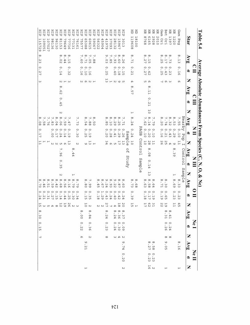
Table 5.4
Average A
bsolute Abundances From
Species (C, N
, O, &
Ne)
C II
C III
N II
N III
O II
Ne I
Ne II
Star
Avg
σ N
A
vg σ
NA
vgσ
NA
vgσ
NA
vgσ
NA
vgσ
NA
vgσ
NNearby
Pop
IControl
Sample
Gam
Peg
8.13
0.16
67.55
0.10
11
8.33
0.23
45
8.16
1HR
1220
8.53
0.29
98.39
18.69
0.23
11
HR
1397
8.73
0.23
38.32
0.43
48.41
0.24
8Bet
Ori
8.17
0.43
67.74
0.21
25
8.30
0.65
19
8.31
0.26
89.05
1Gam
Ori
8.25
0.25
78.20
0.16
26
8.71
0.19
22
HR
2010
HR
2928
7.79
0.10
11
8.64
0.19
31
8.58
0.23
2HR
6165
8.15
0.42
68.11
0.21
10
8.14
0.20
28
8.08
0.14
13
8.58
0.17
62
8.27
0.23
16
HR
8768
8.27
0.27
57.62
0.10
10
8.63
0.18
17
PAGB
Control
Sample
HD
18100
8.68
1HD
119608
8.71
0.21
48.57
18.24
0.24
10
8.73
0.39
15
Sample
of
Study
HIP
3013
8.26
0.15
57.71
0.26
13
8.60
0.24
20
8.37
0.09
29.74
0.20
2HIP
15967
8.60
0.18
98.25
0.29
17
8.87
0.42
18
8.36
0.30
4HIP
28132
7.93
0.40
28.29
0.41
59.22
0.40
48.24
0.24
3HIP
37093
7.85
18.10
0.28
68.93
0.24
7HIP
41979
9.03
0.25
13
8.85
0.20
34
9.24
0.43
27
8.24
0.23
8HIP
45904
8.67
1.29
2HIP
56322
8.45
0.18
2HIP
59067
7.88
18.50
1HIP
60615
7.05
0.16
27.88
0.19
13
7.99
0.35
28.84
0.36
2HIP
65388
8.71
0.10
68.54
0.25
98.80
0.15
10
9.21
1HIP
75577
7.60
0.16
28.00
0.22
6HIP
76161
7.73
0.30
28.79
0.34
3HIP
77131
8.44
18.79
0.30
2HIP
77716
8.15
0.32
37.47
0.19
13
8.16
0.25
26
HIP
79649
8.44
17.59
0.14
68.56
0.44
19
HIP
81153
8.02
0.14
28.62
0.45
28.06
0.24
57.96
0.35
28.68
0.14
12
HIP
96130
8.04
0.17
28.42
0.15
8HIP
98136
7.83
0.00
28.59
0.27
4HIP
107027
7.76
18.51
0.31
5HIP
109051
7.58
18.46
0.21
3HIP
115729
8.23
0.27
38.08
0.17
11
8.70
0.24
15
8.30
0.15
7

Table 5.5
Average A
bsolute Abundances From
Species (Mg, A
l, Si, P, & S)
Mg II
Al II
Al III
Si II Si III
Si IV
P III S II
S III A
r II
Star A
vgσ
N A
vg N A
vg σ
NA
vgσ
NA
vgσ
NA
vgσ
NA
vg NA
vg σ
NA
vgσ
NA
vgσ
NNearby
Pop
IControl
Sample
GamPeg
7.530.07
35.960.02
27.190.22
45.03
17.120.21
96.720.43
56.660.2510
HR1220
6.93
17.570.06
310.08
17.200.16
2HR1397
7.290.09
46.00
16.53
17.400.16
57.220.1915
6.700.01
2BetOri
7.530.16
26.65
16.040.33
48.330.78
47.020.39
67.170.22316.530.84
26.350.34
7GamOri
6.520.33
36.82
17.480.35
87.440.25
66.920.23
26.440.08
4HR2010
7.570.06
36.47
17.590.16
37.970.46
3HR2928
5.890.17
27.320.02
36.990.39
56.820.07
2HR4187
7.540.03
38.29
1HR6165
8.190.46
26.400.14
47.490.32
77.210.06
45.43
19.230.52
26.980.41
68.190.39
3NuCap
7.550.07
36.48
18.110.10
3HR8404
7.490.07
46.38
17.290.00
27.410.32
3HR8768
7.340.01
26.08
16.200.23
37.270.06
35.23
16.990.17
96.790.06
26.530.14
5
BHB
Control
Sample
HD60778
6.66
16.470.13
210.05
1HD74721
6.570.18
2
PAGB
Control
Sample
HD18100
6.830.23
26.740.14
2HD44179
6.35
1HD119608
7.370.42
48.030.12
46.900.25
2
Sample
of
Study
HIP1214
8.51
1HIP1511
8.37
1HIP3013
7.380.01
26.360.21
26.96
17.420.28
47.070.25
77.04
16.460.45
2HIP6727
7.260.07
4HIP123207.79
1HIP159677.870.37
26.661
6.200.33
37.500.18
57.920.30
77.160.38147.74
16.830.39
5HIP161307.38
16.571
7.21
17.05
17.510.89
2HIP28132
6.260.12
26.800.27
37.120.25
46.910.35
48.681.65
2HIP37093
6.560.39
37.680.32
47.58
17.03
1HIP419797.380.07
36.490.53
56.730.30
57.710.13
65.65
17.150.19257.560.33
46.730.20
5HIP45904
6.600.30
38.710.11
26.03
1HIP48394
6.54
16.21
1HIP52906
6.14
17.05
16.970.06
2HIP55461
7.18
1HIP56322
6.97
18.63
17.53
1HIP580467.04
1HIP590677.080.29
27.080.12
3HIP59955
7.490.27
2HIP60615
6.04
17.080.19
36.550.38
27.590.30
5

Table 5.5 (continued)
Mg II
Al II
Al III
Si II
Si III Si IV
P III
S II S III
Ar II
Star
Avg
σ N
Avg N
Avg
σ N
Avg
σN
Avg
σ N
Avg
σN
Avg
N A
vg σ
NA
vgσ
NA
vgσ
NHIP61800
6.05
1HIP65388
7.450.08
36.350.14
27.310.30
37.450.24
77.330.20
36.910.38
3HIP66291
7.800.26
3HIP69247
6.68
17.13
1HIP75577
6.900.2713
8.59
1HIP76161
5.960.37
27.230.05
3HIP77131
8.700.46
2HIP77716
5.410.41
37.070.01
37.52
16.280.12
26.78
1HIP79649
6.040.17
26.930.07
37.070.13
2HIP81153
6.930.38
37.720.06
47.64
16.980.10
4HIP96130
6.30
17.460.12
2HIP98136
7.650.35
37.130.21
2HIP107027
7.510.17
36.78
1HIP109051
7.030.18
36.99
1HIP111396
8.16
1HIP1127907.43
17.67
1HIP114569
7.680.21
37.80
1HIP115729
6.051
6.320.08
36.82
17.390.21
47.000.26
67.180.24
27.00
1

Table 5.6
Average A
bsolute Abundances From
Species (Sc, Ti, C
r, Fe, Y, &
Ba)
Sc II T
i II C
r II Fe I
Fe II Fe III
Y II
Ba II
Star
Avg
σ N
A
vg σ
NA
vg σ
NA
vg σ
N
Avg
σ N
A
vg σ
NA
vg σ
NA
vg N
Nearby
Pop
IControl
Sample
Gam
Peg
7.210.29
4HR
1220
8.02
1HR
1397
5.531.24
25.350.11
27.080.1819
Bet
Ori
8.590.13217.570.57
2Gam
Ori
7.74
1HR
2010
3.360.23
45.070.28225.790.27
97.530.20
97.360.2730
3.65
1HR
2928
7.120.04
2HR4187
2.62
15.160.27276.040.35
67.580.23137.500.3122
3.400.22
23.281
HR
6165
7.220.00
2Nu
Cap
3.170.23
55.010.23315.880.22
97.420.20147.440.2828
2.661
HR
8404
2.780.20
74.860.26395.720.16
97.430.15237.310.1432
2.27
12.761
HR
8768
7.170.37
47.360.08
2BHB
Control
Sample
HD
60778
2.460.15
64.330.26304.600.14
66.590.17146.420.1923
1.271
HD
74721
2.060.05
64.170.24264.470.14
46.190.13166.270.1222
0.911
PAGB
Control
Sample
HD
44179
4.06
1HD
1052621.59
13.790.19204.030.28
35.780.05
66.040.1418
Sample
of
Study
HIP
1214
4.85
16.910.40
3HIP
1511
2.650.25
64.270.26244.450.24
56.920.23126.000.2012
1.561
HIP
3013
8.14
1HIP
6727
2.900.27
54.880.27305.430.26
67.690.20217.050.2126
2.31
12.081
HIP
11844
5.15
15.00
16.900.18
8HIP
15967
8.360.42
2HIP
16130
6.580.67
27.210.29
6HIP
28132
7.72
1HIP
41979
8.030.18
3HIP
58046
7.21
1HIP
59067
7.470.31
3HIP
59955
6.810.57
5

Table 5.6 (continued)
Sc II T
i II C
r II Fe I
Fe II Fe III
Y II
Ba II
Star A
vg σ
N
Avg
σ N
A
vg σ
N
Avg
σ N
A
vg σ
N
Avg
σ N
A
vgσ
NA
vgN
HIP
61800
7.160.20
2HIP
63591
6.44
17.750.13
27.330.34
4HIP
65388
8.020.49
4HIP
69247
4.280.09
24.780.08
26.740.1917
HIP
76161
7.580.34
2HIP
107027
6.75
1HIP
109051
HIP
111396
5.530.32
35.870.48
27.400.3315
HIP
115729
8.30
1HIP
1165601.13
13.350.35173.840.02
25.250.05
55.400.1011

Table 5.7
Average A
bsolute Abundances of the N
earby Pop I Control Sam
ple Versus O
thers
C
N
O
Ne
Mg
Al
Si S
Ar
Fe Sun(1)
8.52
7.92
8.83
8.08
7.58
6.47
7.55
7.33
6.40
7.50
This
Study
8.28
7.98
8.55
8.35
7.56
6.30
7.36
7.25
6.58
7.40
DKBS
BStars(6)
8.18
7.75
8.62
7.65
6.15
7.36
7.27
7.35
BSuper
Giants(2)
7.82
7.38
8.68
7.09
5.86
7.14
DKB
Cep
OB1(5)
8.17
7.62
8.61
7.21
7.24
G&L
BDwarfs(4)
8.20
7.81
8.68
7.97
6.45
7.58
7.21
7.72
Kilian
BDwarfs(3)
8.22
7.78
8.52
7.38
5.81
6.81
1=
Grevesse
&Suaval
(1998)
2=
Vrancken
et
al.
(2000)
3=
Kilian
(1992)
4=
Gies
&Lambert
(1992)
5=
Daflon,
Cunha,
&Becker
(1999)
6=
Daflon
et
al.
(2001)

130
The absolute abundances of the nearby Population I B star control sample
compare favorably with results from a variety of other studies (See Table 5.7). The
relative abundances are calculated from line by line differences with an “average star”
built from the nearby Population I B star abundance control sample.
5.4.1 Building An Average Star
It is easiest to measure the relative abundances between two stars with the same
atmospheric parameters because then the only variable which they do not have in
common is their composition. In a perfect universe there would be one star that we could
observe as a standard which all other stars could be compared to (i.e. the Sun). However
in reality, stars cover such a large range of effective temperatures that the atomic
transitions and processes in a star on the cool end of the scale have almost no application
in a star on the hot end. Unfortunately there is even a large range of physical conditions
in B stars (Teff= 10000 K to 35000 K). The spectrum of an early type B star bears almost
no resemblance to a late type B star, save for the ever present hydrogen and helium lines.
In order to do a good job of measuring the relative compositions of B stars, one must find
a way to tie the abundances of these stars together over the wide range of parameter space
that they occupy. In this study, this is accomplished by building an “average star” from
the control sample.
The control sample of nearby Population I B stars is drawn from a population that
is for the most part chemically homogeneous (Kilian 1992; Gies & Lambert 1992). In
this case one assumes that differences in the equivalent width measured for a given line
in each of these stars are not due to differences in composition of the atmospheres but

131
primarily caused by differences in the structure of the stellar atmosphere as defined by
the photospheric parameters. Therefore, transitions that give abundances which show
trends with respect to temperature or large random spreads are dropped from the analysis
as unreliable indicators of relative abundance.
In the course of generating a list of reliable atomic transitions from the nearby
Population I control sample in this manner, it became apparent that some atomic species
were reliable indicators of abundance over part of the temperature range, but then became
less reliable outside of that range. To compensate for this, rules were adopted which
restricted the use of lines from some species only over a specified range of effective
temperatures (Table 5.8).
Table 5.8 Teff Limits Imposed on Species in the Abundance Analysis
Species Upper
Limit (K) Lower
Limit (K)C III 25000N III 25000Ne II 17000Al II 20000Si III 15000Si II 15000S IV 25000S III 13000Ar II 12000Ti II 15000Cr II 15000Fe I 11000Fe II 18000

132
Some lines were measured in only one star in the nearby Population I control
sample. Those lines in this situation which yield abundances that are consistent with
other reliable lines in that star were given the benefit of the doubt and included in the line
list. In a perfect world there would have been enough lines to choose from that one
would not have to take a chance that some of these lines measured in only one star were
unreliable. However there are not a large number spectral lines in most B stars so it is
pragmatic to keep a line in the list until it has proven itself unreliable. The list of lines
selected in this manner appears in Table 5.1.
In this study, the reference point that abundances are measured against is not a
single star, but an “average star” manufactured using the average abundances for each
line from all the stars in the Pop I control sample (Table 5.9). Relative stellar abundances
are calculated on a line by line basis as the difference with respect the average absolute
abundance measured for that line in the Pop I control sample (Tables 5.10 through 5.12).
Table 5.9 Average Normal Star
Table 5.9 Species λλλλ0000====((((Å) Avg σ NC II 4313.106 8.39 0.02 2C II 4318.606 8.62 0.09 3C II 4374.272 8.19 0.16 3C II 4376.562 8.11 0.30 2C II 4411.200 8.26 0.10 4C II 4411.520 7.99 0.18 2C II 4637.630 8.54 1C II 5133.280 8.30 0.47 2C II 5143.490 8.22 0.00 1C II 5145.160 8.04 0.11 2C II 5151.090 7.98 0.40 2C II 6098.510 8.64 1C II 6578.050 8.21 0.48 4C II 6582.880 8.17 0.35 4C III 4186.900 7.90 1C III 4325.560 8.32 1C III 4515.811 7.94 1C III 4516.788 7.92 1C III 4647.418 8.35 1C III 4650.246 8.36 1
Table 5.9 Species λλλλ0000====((((Å) Avg σ NC III 4659.058 8.34 1C III 4663.642 8.14 1C III 5695.920 7.90 1C III 5826.420 7.92 1N II 4227.750 7.89 0.12 6N II 4241.800 7.88 0.09 7N II 4427.236 8.18 0.11 4N II 4427.964 8.30 1N II 4432.730 7.88 0.23 7N II 4433.480 7.87 0.02 3N II 4441.990 7.96 0.34 4N II 4447.030 7.89 0.16 7N II 4507.560 7.93 0.13 4N II 4530.410 7.67 0.16 6N II 4601.478 7.99 0.08 7N II 4607.153 7.83 0.05 6N II 4613.868 8.05 0.11 5N II 4621.393 7.84 0.13 3N II 4630.539 7.88 0.21 6N II 4643.086 8.06 0.13 5

133
Table 5.9 Species λλλλ0000====((((Å) Avg σ NN II 4654.531 8.45 0.02 2N II 4674.908 8.53 1N II 4678.100 8.18 0.05 2N II 4694.700 8.14 1N II 4779.722 8.07 0.16 2N II 4788.138 7.93 0.04 2N II 4803.287 7.94 0.16 2N II 4810.299 8.04 1N II 4895.117 8.03 0.32 2N II 5002.703 8.39 1N II 5005.150 7.82 0.00 2N II 5007.328 7.96 1N II 5010.621 7.96 0.17 2N II 5045.099 8.06 0.03 2N II 5666.629 7.87 0.07 3N II 5676.017 7.99 0.04 3N II 5679.558 8.08 0.12 3N II 5686.213 7.95 0.12 2N II 5710.766 8.15 0.15 3N II 5747.300 8.54 0.11 2N II 5941.654 8.24 1N II 6167.755 8.35 1N II 6173.312 8.55 1N II 6610.562 7.76 1N III 4195.740 7.93 1N III 4200.070 8.07 1N III 4215.770 8.00 1N III 4379.110 8.15 0.12 2N III 4514.850 8.24 1N III 4518.140 8.15 1N III 4523.560 8.16 1N III 4527.860 8.30 1N III 4530.860 8.24 1N III 4534.580 8.21 1N III 4546.330 8.01 1N III 4634.130 7.93 1N III 4640.640 7.94 1O II 4185.440 8.44 1O II 4189.790 8.37 0.27 2O II 4192.512 8.52 0.00 2O II 4196.697 8.55 0.18 2O II 4274.243 8.42 0.16 2O II 4275.529 8.24 0.13 5O II 4277.427 8.52 0.13 3O II 4277.894 8.73 0.02 3O II 4281.313 8.18 0.08 3O II 4282.961 8.31 0.32 3O II 4283.721 8.70 0.10 3O II 4291.254 8.86 0.12 3O II 4294.782 8.84 0.47 5O II 4295.919 8.12 1O II 4303.832 8.57 0.08 4O II 4307.232 8.71 0.28 4O II 4309.007 8.48 0.12 3
Table 5.9 Species λλλλ0000====((((Å) Avg σ NO II 4312.100 8.58 0.10 3O II 4313.442 8.12 0.11 3O II 4315.826 8.71 0.18 2O II 4317.139 8.57 0.15 5O II 4317.696 8.39 0.09 2O II 4319.630 8.46 0.26 6O II 4325.761 8.73 0.18 4O II 4327.460 8.43 0.05 3O II 4328.591 8.40 0.01 2O II 4331.857 8.32 0.02 2O II 4336.859 8.12 0.14 3O II 4345.560 8.25 0.16 3O II 4347.413 8.43 0.24 3O II 4351.260 8.51 0.19 3O II 4358.442 8.78 0.23 2O II 4366.895 8.55 0.12 6O II 4369.272 8.45 0.14 4O II 4378.428 8.74 0.11 3O II 4395.935 8.80 0.49 3O II 4405.978 8.75 0.00 1O II 4414.899 8.41 0.30 6O II 4416.975 8.69 0.23 6O II 4443.010 8.50 0.04 3O II 4448.191 8.55 0.20 4O II 4452.378 8.67 0.10 5O II 4465.407 8.74 0.03 3O II 4467.465 8.50 1O II 4487.712 8.41 0.17 2O II 4491.222 8.51 0.66 4O II 4590.974 8.46 0.31 7O II 4596.177 8.69 0.11 6O II 4602.129 8.34 0.14 3O II 4609.436 8.39 0.21 4O II 4610.202 8.90 1O II 4638.856 8.53 0.21 4O II 4649.135 8.28 0.39 3O II 4650.838 8.38 0.42 3O II 4661.632 8.53 0.36 5O II 4673.733 8.84 0.04 2O II 4676.235 8.26 0.35 2O II 4677.065 8.92 1O II 4690.888 8.52 1O II 4691.419 8.49 1O II 4698.437 8.45 1O II 4699.218 8.52 1O II 4701.179 8.64 0.49 2O II 4701.712 8.65 1O II 4703.161 8.58 0.36 3O II 4705.346 8.46 0.08 2O II 4710.009 8.68 0.21 2O II 4906.830 8.74 1O II 4941.072 8.61 1O II 4943.005 8.66 1O II 5159.941 9.22 1

134
Table 5.9 Species λλλλ0000====((((Å) Avg σ NO II 5206.651 8.94 1O II 6641.031 8.70 1Ne I 5852.488 8.51 0.08 2Ne I 6143.062 8.37 0.07 2Ne I 6163.594 8.14 0.11 2Ne I 6334.428 8.57 0.22 2Ne I 6382.991 8.26 0.04 2Ne I 6506.528 8.05 0.19 2Ne I 6598.953 8.26 0.03 2Ne I 6717.043 8.73 0.14 2Ne II 4290.602 9.05 1Ne II 4379.552 8.22 1Ne II 4391.991 8.08 1Ne II 4397.990 8.62 1Ne II 4409.299 8.24 0.08 3Ne II 4412.591 8.17 1Ne II 4413.109 8.11 1Ne II 4429.640 8.16 1Ne II 4432.303 7.93 1Ne II 4439.253 8.27 1Ne II 4439.462 8.64 1Ne II 4457.049 8.48 0.16 2Ne II 4457.355 8.36 1Ne II 4498.924 8.61 1Ne II 4499.117 8.55 1Ne II 4522.720 8.00 1Ne II 4569.057 8.17 1Mg II 4384.640 7.44 0.09 5Mg II 4390.560 7.51 0.07 8Mg II 4427.990 7.65 0.14 6Mg II 4433.990 7.52 0.12 7Al II 4663.046 6.34 0.00 6Al III 4512.565 5.99 0.16 6Al III 4528.945 6.47 1Al III 4529.189 6.23 0.11 7Al III 5696.604 6.52 0.10 3Al III 5722.730 6.51 0.07 3Si II 4621.418 7.34 0.01 2Si II 4621.722 7.23 0.16 2Si II 5041.024 7.30 0.38 2Si II 5055.984 8.25 1Si II 5957.560 7.65 0.03 2Si II 5978.930 7.57 0.25 3Si II 6371.355 8.17 0.64 3Si III 4552.622 7.33 0.08 7Si III 4553.997 7.71 0.07 2Si III 4567.840 7.29 0.11 7Si III 4574.757 7.30 0.13 7Si III 4683.020 7.67 1Si III 4716.654 7.18 0.71 3Si III 4813.330 7.18 1Si III 4828.960 6.97 0.07 2Si III 5114.116 8.09 1Si III 5739.730 7.44 0.20 3
Table 5.9 Species λλλλ0000====((((Å) Avg σ NSi IV 4314.102 7.21 1Si IV 4631.240 7.30 1Si IV 4654.320 7.15 1Si IV 6667.570 7.19 1P III 4246.680 5.23 0.00 3S II 4259.146 7.70 1S II 4267.762 7.44 0.15 3S II 4269.760 7.06 0.21 4S II 4278.540 7.00 0.15 4S II 4282.630 7.29 0.33 5S II 4291.450 8.77 0.20 2S II 4294.402 6.94 0.07 5S II 4432.410 7.33 1S II 4456.430 7.92 0.22 3S II 4463.580 7.35 0.16 5S II 4483.420 7.38 0.13 3S II 4486.660 7.30 0.10 2S II 4524.680 7.44 0.01 2S II 4524.950 7.41 0.12 7S II 4552.380 8.05 1S II 4656.740 7.00 0.06 3S II 4716.230 7.30 1S II 4792.020 6.97 1S II 4815.520 7.23 0.27 2S II 4824.070 7.30 1S II 4835.850 7.63 1S II 4885.630 7.45 0.06 2S II 4917.150 7.42 0.01 2S II 4925.320 7.56 1S II 4942.470 7.20 1S II 4991.940 7.32 1S II 5009.540 7.20 1S II 5014.030 7.42 0.12 2S II 5027.190 7.23 1S II 5032.410 7.20 0.30 2S II 5103.300 6.80 1S II 5142.330 7.19 1S II 5606.151 6.94 0.11 2S II 5616.633 7.06 1S II 5647.020 7.52 0.11 3S II 5660.001 7.67 0.17 3S II 5664.773 7.10 1S II 5819.254 7.45 1S III 4253.499 6.66 0.26 6S III 4284.990 6.76 0.22 4S III 4332.653 6.74 0.18 2S III 4361.468 6.88 0.27 6S III 4364.661 6.78 0.04 2S III 4439.870 7.60 0.12 3S III 4467.716 7.16 1Ar II 4228.158 6.67 0.26 3Ar II 4331.199 7.17 0.01 3Ar II 4370.753 7.20 0.18 2Ar II 4371.329 6.86 0.05 2

135
Table 5.9 Species λλλλ0000====((((Å) Avg σ NAr II 4400.986 6.58 0.06 2Ar II 4426.001 6.39 0.12 5Ar II 4430.189 6.41 0.13 2Ar II 4448.879 7.91 0.11 2Ar II 4545.052 6.70 1Ar II 4579.349 6.60 0.20 2Ar II 4589.898 6.59 0.08 2Ar II 4735.905 6.26 1Ar II 4806.020 6.22 0.27 2Ar II 4847.809 6.61 0.37 2Ar II 4879.863 6.31 0.27 2Sc II 4246.822 2.82 0.13 4Sc II 4314.083 3.28 0.17 3Sc II 4320.732 3.14 0.17 3Sc II 4324.996 2.99 0.08 3Sc II 4374.457 2.78 1Sc II 4400.389 2.95 0.06 2Sc II 4670.407 3.21 1Ti II 4171.920 4.94 1Ti II 4174.050 4.66 1Ti II 4184.303 5.04 1Ti II 4287.880 5.20 0.11 4Ti II 4290.220 5.05 0.06 4Ti II 4294.090 5.04 0.04 4Ti II 4300.049 4.69 0.28 5Ti II 4301.920 4.79 0.02 4Ti II 4307.863 5.27 0.09 4Ti II 4312.870 4.96 0.04 4Ti II 4314.970 4.95 0.06 4Ti II 4316.800 4.66 0.04 2Ti II 4320.960 5.13 0.29 3Ti II 4337.880 4.42 0.18 2Ti II 4350.850 4.53 0.20 2Ti II 4367.650 5.37 0.08 3Ti II 4391.040 5.28 1Ti II 4394.051 4.83 0.06 2Ti II 4395.850 4.97 2Ti II 4399.790 4.93 0.01 4Ti II 4407.680 5.23 0.16 4Ti II 4409.220 4.96 0.30 2Ti II 4411.100 5.34 0.07 4Ti II 4417.720 5.03 0.03 4Ti II 4418.330 4.92 0.14 2Ti II 4421.950 5.08 0.10 3Ti II 4441.730 4.99 1Ti II 4443.794 4.65 0.14 4Ti II 4444.558 4.92 0.09 3Ti II 4450.482 4.92 0.08 3Ti II 4464.460 5.52 0.28 5Ti II 4468.507 4.67 0.12 4Ti II 4488.340 5.24 0.08 4Ti II 4501.273 4.76 0.08 4Ti II 4529.480 5.46 0.06 4Ti II 4533.970 5.20 0.09 4
Table 5.9 Species λλλλ0000====((((Å) Avg σ NTi II 4549.610 5.57 1Ti II 4563.770 4.93 0.05 4Ti II 4571.960 4.97 0.13 4Cr II 4539.610 6.22 0.12 4Cr II 4555.010 5.81 0.02 4Cr II 4558.660 5.68 0.16 5Cr II 4565.770 6.18 0.13 4Cr II 4588.220 5.50 0.14 5Cr II 4592.070 5.70 0.02 4Cr II 4616.640 5.61 0.04 3Cr II 4618.820 5.82 0.06 3Cr II 4634.100 5.85 0.02 3Fe I 4175.640 7.38 1Fe I 4181.750 7.29 1Fe I 4184.890 7.50 1Fe I 4187.040 7.46 1Fe I 4187.790 7.95 1Fe I 4202.030 7.58 0.09 3Fe I 4233.600 7.30 1Fe I 4235.940 7.48 0.07 3Fe I 4238.810 7.67 1Fe I 4247.430 7.46 0.10 3Fe I 4250.120 7.54 0.15 3Fe I 4250.790 7.51 0.11 3Fe I 4260.473 7.48 0.04 4Fe I 4271.150 7.42 0.07 3Fe I 4271.760 7.32 0.08 4Fe I 4282.400 7.68 0.09 3Fe I 4325.760 7.13 1Fe I 4369.770 7.34 1Fe I 4383.540 7.15 0.14 4Fe I 4404.750 7.33 0.05 4Fe I 4415.120 7.48 0.05 4Fe I 4466.550 7.50 0.10 2Fe I 4494.560 7.67 0.10 3Fe I 4528.610 7.72 0.15 4Fe II 4173.450 7.05 1Fe II 4178.860 7.25 0.01 2Fe II 4233.170 7.48 0.25 5Fe II 4258.160 7.46 0.13 5Fe II 4273.320 7.76 0.05 5Fe II 4296.570 7.63 0.05 6Fe II 4303.170 7.40 0.12 6Fe II 4351.760 7.20 0.15 6Fe II 4369.400 7.65 0.13 4Fe II 4384.330 7.26 1Fe II 4413.600 7.46 0.18 4Fe II 4416.820 7.26 0.12 5Fe II 4472.920 7.40 0.33 4Fe II 4489.190 7.63 0.13 6Fe II 4491.400 7.50 0.04 6Fe II 4508.280 7.25 0.11 7Fe II 4515.340 7.45 0.05 6Fe II 4520.230 7.48 0.07 6

136
Table 5.9 Species λλλλ0000====((((Å) Avg σ NFe II 4522.630 7.02 0.14 5Fe II 4541.520 7.67 0.03 6Fe II 4549.210 7.65 1Fe II 4549.470 7.78 0.41 7Fe II 4555.890 7.35 0.07 6Fe II 4576.330 7.68 0.08 6Fe II 4582.840 7.43 0.09 4Fe II 4583.830 7.45 0.22 7Fe II 4620.510 7.69 0.01 4Fe II 4629.340 7.36 0.08 5Fe II 4635.330 7.75 0.22 6Fe II 4656.970 7.59 0.13 3Fe II 4666.750 7.77 0.07 4
Table 5.9 Species λλλλ0000====((((Å) Avg σ NFe II 4670.170 7.71 0.23 3Fe II 4731.440 8.28 0.13 2Fe II 5197.560 8.27 1Fe II 5961.710 7.37 1Fe III 4222.271 7.52 0.42 3Fe III 4296.851 7.38 0.19 5Fe III 4310.355 7.16 0.08 4Fe III 4372.536 8.02 1Fe III 4372.823 7.04 1Y II 4177.536 2.96 0.52 2Y II 4309.622 3.24 1Y II 4422.588 3.55 1Ba II 4554.036 2.90 0.00 3
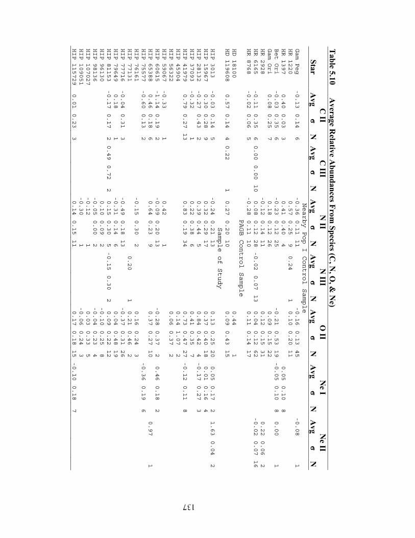
Table 5.10 A
verage Relative A
bundances From Species (C
, N, O
, & N
e)
C II
C III
N II
N III
O II
Ne I
Ne II
Star
Avg
σ N
A
vg σ
NA
vg σ
NA
vg σ
NA
vg σ
NA
vg σ
NA
vg σ
NNearby
Pop
IControl
Sample
Gam
Peg
-0.13
0.14
6-0.36
0.11
11
-0.16
0.13
45
-0.08
1HR
1220
0.57
0.25
90.24
10.10
0.20
11
HR
1397
0.40
0.03
30.41
0.40
40.05
0.10
8Bet
Ori
-0.03
0.35
6-0.23
0.12
25
-0.21
0.53
19
-0.05
0.10
80.00
1Gam
Ori
0.08
0.25
70.18
0.12
26
0.09
0.15
22
HR
2928
-0.12
0.14
11
0.12
0.15
31
0.22
0.06
2HR
6165
-0.11
0.35
60.00
0.00
10
0.08
0.12
28
-0.02
0.07
13
0.04
0.12
62
-0.02
0.07
16
HR
8768
-0.02
0.06
5-0.28
0.11
10
0.11
0.14
17
PAGB
Control
Sample
HD
18100
0.44
1HD
119608
0.57
0.14
40.22
10.27
0.20
10
0.09
0.43
15
Sample
of
Study
HIP
3013
-0.03
0.14
5-0.24
0.21
13
0.13
0.25
20
0.05
0.17
21.63
0.04
2HIP
15967
0.30
0.28
90.32
0.29
17
0.37
0.40
18
0.01
0.16
4HIP
28132
-0.27
0.43
20.39
0.44
50.84
0.42
4-0.17
0.27
3HIP
37093
-0.32
10.22
0.38
60.41
0.35
7HIP
41979
0.79
0.27
13
0.83
0.19
34
0.73
0.47
27
-0.12
0.11
8HIP
45904
0.14
1.07
2HIP
56322
0.06
0.37
2HIP
59067
-0.33
10.42
1HIP
60615
-1.14
0.19
2-0.09
0.20
13
-0.28
0.37
20.46
0.18
2HIP
65388
0.46
0.18
60.64
0.23
90.37
0.27
10
0.97
1HIP
75577
-0.60
0.13
2-0.36
0.19
6HIP
76161
-0.15
0.30
20.16
0.24
3HIP
77131
0.20
10.21
0.46
2HIP
77716
-0.04
0.31
3-0.49
0.18
13
-0.37
0.31
26
HIP
79649
0.18
1-0.31
0.14
60.04
0.48
19
HIP
81153
-0.17
0.17
20.49
0.72
20.15
0.30
5-0.15
0.30
20.09
0.22
12
HIP
96130
0.10
0.09
2-0.10
0.25
8HIP
98136
-0.05
0.00
2-0.04
0.23
4HIP
107027
-0.12
10.03
0.33
5HIP
109051
-0.30
1-0.06
0.24
3HIP
115729
0.01
0.23
30.14
0.15
11
0.17
0.18
15
-0.10
0.18
7
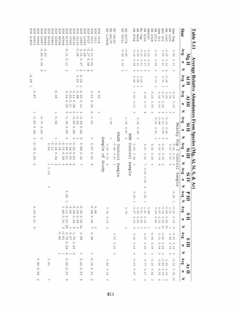
Table 5.11
Average R
elative Abundances From
Species (Mg, A
l, Si, S, & A
r)
Mg II
Al II
Al III
Si II Si III
Si IV
P IIIS II
S III A
r II Star
Avg
σ N
A
vg N
A
vg σ
NA
vg σ
NA
vg σ
NA
vgσ
N
Avg
NA
vg σ
NA
vg σ
NA
vg σ
NNearby
Pop
IControl
Sample
GamPeg
0.04
0.11
3-0.16
0.15
2-0.22
0.03
4-0.20
1-0.12
0.16
9-0.21
0.10
5-0.19
0.32
10
HR1220
0.70
10.27
0.07
31.31
10.48
0.09
2
HR1397
-0.25
0.12
4-0.34
10.30
1-0.19
0.25
5-0.05
0.24
15
0.22
0.12
2
BetOri
0.05
0.21
20.31
1-0.27
0.09
40.51
0.56
4-0.23
0.39
6-0.15
0.30
31
-0.25
0.69
2-0.09
0.19
7
GamOri
0.18
0.03
3-0.48
10.13
0.19
80.07
0.12
60.15
0.38
20.06
0.22
4
HR2010
0.01
0.09
30.13
1-0.20
0.43
30.59
0.54
3
HR2928
-0.22
0.00
20.02
0.04
3-0.04
0.09
5-0.10
0.42
2
HR4187
-0.02
0.10
30.88
1
HR6165
0.60
0.37
20.09
0.17
40.07
0.21
70.00
0.00
40.20
11.43
0.35
20.07
0.09
60.77
0.17
3
NuCap
-0.01
0.11
30.14
10.51
0.45
3
HR8404
-0.04
0.12
40.04
10.00
0.08
20.05
0.06
3
HR8768
-0.14
0.04
2-0.26
1-0.03
0.13
3-0.04
0.04
30.00
1-0.27
0.30
90.02
0.10
2-0.03
0.07
5
BHB
Control
Sample
HD60778
-0.85
1-1.30
0.81
22.75
1
HD74721
-0.94
0.18
2
PAGB
Control
Sample
HD18100
-0.48
0.21
20.03
0.21
2
HD44179
-1.90
1
HD119608
0.02
0.31
40.74
0.19
40.64
0.19
2
Sample
of
Study
HIP1214
2.52
1HIP1511
0.96
1HIP3013
-0.130.02
20.110.16
2-1.21
10.070.21
4-0.280.25
70.38
1-0.160.11
2HIP6727
-0.270.08
4HIP12320
0.28
1HIP15967
0.350.37
20.32
1-0.050.13
3-0.290.42
50.680.34
7-0.050.3614
1.08
10.220.53
5HIP16130-0.06
10.23
10.98
1-0.25
10.380.99
2HIP28132
-0.110.08
2-0.900.55
3-0.220.20
4-0.280.34
41.761.29
2HIP37093
0.220.11
30.340.25
40.06
10.37
1HIP41979-0.110.11
30.140.32
5-1.060.45
50.460.21
60.42
1-0.130.2325
0.790.28
40.220.23
5HIP45904
-0.700.29
31.490.33
2-0.63
1HIP48394
-0.75
1-0.45
1HIP52906
-0.38
1-0.52
1-0.340.04
2HIP55461
-0.11
1HIP56322
0.00
11.33
11.31
1HIP58046-0.47
1HIP59067-0.400.34
2-0.710.43
3HIP59955
0.940.05
2HIP60615
-0.47
1-0.830.34
3-0.760.20
20.190.31
5HIP61800
-0.29
1

Table 5.11 (continued)
Mg II
Al II
Al III
Si II Si III
Si IV
P III S II
S III A
r IIStar
Avg
σ N
A
vg N
A
vg σ
NA
vg σ
NA
vg σ
NA
vgσ
NA
vg N
Avg
σ N
Avg
σ N
Avg
σ N
HIP65388
-0.040.10
30.240.03
20.000.28
30.110.25
70.590.14
30.250.47
3HIP66291
0.490.24
3HIP69247
-0.83
1-1.04
1HIP75577
-0.410.2713
0.68
1HIP76161
-0.150.20
2-0.080.06
3HIP77131
1.380.43
2HIP77716
-1.010.24
3-0.280.07
30.00
1-0.530.22
2-0.39
1HIP79649
-0.070.00
2-0.380.06
30.360.06
2HIP81153
0.590.14
30.380.05
40.34
10.220.18
4HIP96130
0.31
10.150.09
2HIP98136
0.350.33
30.420.14
2HIP107027
0.200.15
30.12
1HIP109051
-0.280.16
30.33
1HIP111396
1.57
1HIP112790-0.08
10.34
1HIP114569
0.370.23
31.14
1HIP115729
-0.29
10.080.20
3-1.35
10.050.14
4-0.200.23
60.410.08
20.14
1

Table 5.12 A
verage Relative A
bundances From Species (Sc, C
r, Ti, Fe, Y, &
Ba)
Sc II C
r II T
i II Fe I
Fe II Fe III
Y II
Ba II
Star
Avg
σ N
A
vg σ
NA
vgσ
NA
vgσ
NA
vg σ
NA
vgσ
NA
vgσ
NA
vgN
Nearby
Pop
IControl
Sample
Gam
Peg
-0.07
0.16
4
HR
1220
0.00
1
HR
1397
0.42
0.65
2-0.24
0.01
2-0.38
0.14
19
Bet
Ori
0.98
0.31
21
0.12
0.66
2
Gam
Ori
0.22
1
HR
2010
0.31
0.05
40.03
0.10
22
-0.03
0.04
90.06
0.05
9-0.14
0.17
30
0.69
1
HR
2928
-0.15
0.12
2
HR
4187
-0.20
10.14
0.10
27
0.19
0.08
60.10
0.09
13
0.03
0.21
22
0.00
0.00
20.38
1
HR
6165
-0.05
0.16
2
Nu
Cap
0.13
0.08
50.01
0.09
31
0.06
0.04
9-0.04
0.07
14
-0.10
0.18
28
-0.24
1
HR
8404
-0.24
0.22
7-0.14
0.13
39
-0.10
0.16
9-0.06
0.09
23
-0.17
0.15
32
-0.69
1-0.14
1
HR
8768
-0.39
0.29
40.08
0.08
2
PAGB
Control
Sample
HD
44179
-1.76
1
HD
105262
-1.23
1-1.24
0.14
20
-1.60
0.33
3-1.54
0.13
6-1.42
0.17
18
BHB
Control
Sample
HD
60778
-0.53
0.26
6-0.68
0.11
30
-1.13
0.11
6-0.87
0.10
14
-1.15
0.25
23
-1.63
1
HD
74721
-0.93
0.21
6-0.87
0.17
26
-1.20
0.11
4-1.26
0.10
16
-1.19
0.15
22
-1.99
1
Sample
of
Study
HIP
1214
0.20
1-0.70
0.36
3
HIP
1511
-0.34
0.38
6-0.73
0.24
24
-1.25
0.19
5-0.50
0.34
12
-1.39
0.18
12
-1.34
1
HIP
3013
0.12
1
HIP
6727
-0.10
0.35
5-0.13
0.17
30
-0.41
0.14
60.21
0.19
21
-0.39
0.26
26
-0.65
1-0.82
1
hip
11844
-0.12
1-0.50
1-0.54
0.20
8
HIP
15967
1.09
0.27
2
HIP
16130
1.04
0.71
2-0.13
0.33
6
HIP
28132
0.35
1
HIP
41979
0.67
0.06
3
HIP
58046
-0.15
1
HIP
59067
0.12
0.37
3
HIP
59955
-0.56
0.48
5
HIP
61800
-0.41
0.09
2
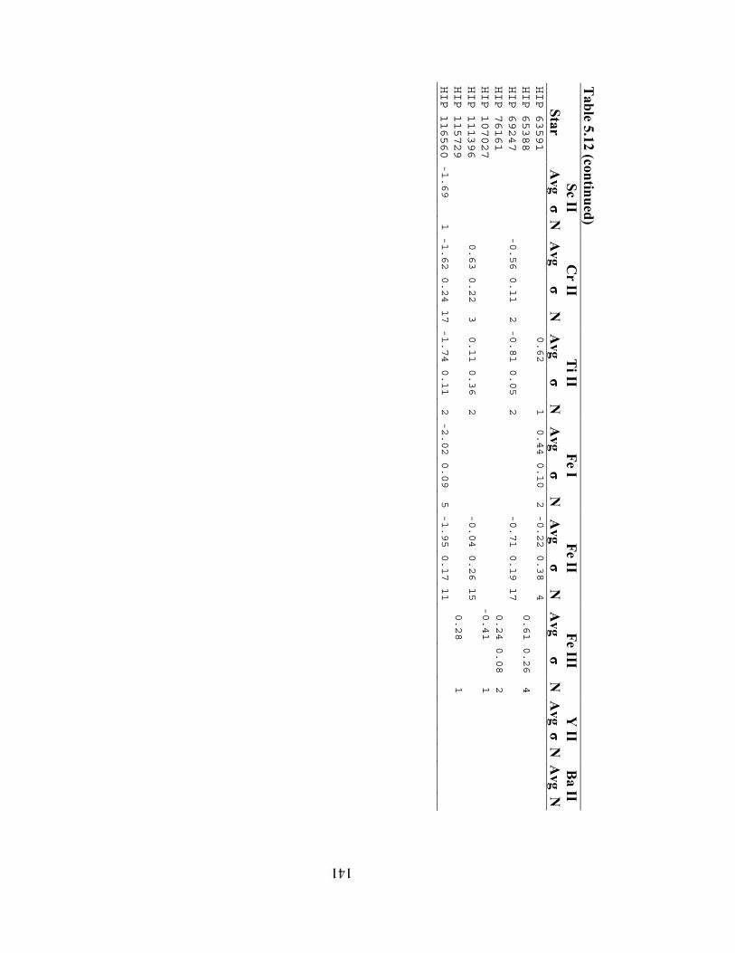
Table 5.12 (continued)
Sc II C
r II T
i II Fe I
Fe II Fe III
Y II
Ba II
Star A
vg σ N
A
vg σ
NA
vg σ
NA
vg σ
NA
vg σ
NA
vg σ
NA
vgσ
NA
vgN
HIP
63591
0.62
10.44
0.10
2-0.22
0.38
4
HIP
65388
0.61
0.26
4
HIP
69247
-0.56
0.11
2-0.81
0.05
2-0.71
0.19
17
HIP
76161
0.24
0.08
2
HIP
107027
-0.41
1
HIP
111396
0.63
0.22
30.11
0.36
2-0.04
0.26
15
HIP
115729
0.28
1
HIP
116560
-1.69
1-1.62
0.24
17
-1.74
0.11
2-2.02
0.09
5-1.95
0.17
11

142
Ideally this method should reduce the standard deviation about the mean
abundance measured from several individual lines in the same star. In an absolute
abundance analysis a line that consistently yields an abundance a few tenths of a dex
above or below the actual composition of the star would enlarge the standard deviation
of measured values. However, this method of measuring relative abundances on a line
by line basis compensates for the offset in the absolute abundance which has the net
effect of reducing the standard deviation of the abundance measured from several lines
in the same star.
In practice the ideal conditions are not always met. The difference between the
standard deviations from the absolute analysis subtracted from the relative analysis are
in Table 5.13. There is a significant improvement in average standard deviations of ten
species (N III, Ne I, Ne II, Al III, Si III, Ti II, Cr II, Fe I, Fe III, Y II). Those species
most improved either are measured from a small list of very well behaved transitions or
are only used over a narrow temperature range. In either of those cases the conditions
are most ideal for relative abundance analysis to remove effects from the atomic data
and atmospheric parameters to first order. All but one of the other species showed no
significant change in precision as a result of relative abundance analysis. The average
standard deviation of Si II in the relative abundance analysis was larger than computed
in the absolute abundance analysis because Si II is very sensitive to changes in
atmospheric parameters (section 5.6.2). Therefore Si II is not well suited for relative
analysis.

143
Table 5.13 Improvement of Abundance Errors by Relative Analysis Avg(1)
Species ∆σ σabs C II -0.02 0.29C III 0.03 0.33N II -0.01 0.22N III -0.07 0.14O II 0.01 0.31Ne I -0.06 0.24Ne II -0.16 0.22Mg II 0.02 0.13Al III -0.13 0.26Si II 0.15 0.27Si III -0.03 0.23S II 0.02 0.30S III -0.10 0.37Ar II -0.01 0.24Sc II -0.02 0.23Ti II -0.14 0.38Cr II -0.10 0.23Fe I -0.05 0.15Fe II -0.01 0.27Fe III -0.07 0.30Y II -0.38 0.62(1) Avg ∆σ is the averagevalue of (σabs – σrel) for agiven species. A negativenumber means that therelative abundance analysisyieled a smaller standarddeviation than the absoluteabundance analysis.
In some stars, abundances were determined from more than one species of
certain elements. In these cases, the elemental ratios and discussion of elemental
abundances will be based on the major ionization species, which is often the one with
the most lines measured. Figure 5.1 shows the distribution of elemental abundances in
the sample of study measured relative to the control sample.

144
Figure 5.1 Relative Abundance Distributions
These are histograms of the relative abundances of carbon, nitrogen, oxygen, silicon, sulfur, and iron for the sample of high latitude B stars. The nearby Pop I control sample is plotted at the top of each histogram for comparison. The dotted vertical lines are the minimum and maximum value in the nearby Pop I control sample.

145
5.4.2 Abundance Ratios
Abundance ratios are helpful for determining the pattern of enhancements and
depletions in a stellar atmosphere. Of primary interest to this study are enhancements
of carbon, nitrogen, oxygen, s-process, α-process, and refractory elements which are
used to distinguish between BHB, PAGB, PPN, and main sequence stars. In order for a
ratio to effectively detect an enhancement, depletion, or lowered measured abundance
of an element it must be compared to another element that is unaffected by the process
that one wishes to test for.
An element which is unaffected by all of these processes would be the ideal
universal referent. Pragmatism dictates that the referent selected must be measurable
over the same range of atmospheric parameters as the element that is being tested for
variation. However, it has proven difficult to identify one element with all these
qualities so instead several different elements are used as referents, each with its own
strengths and weaknesses.
Iron is often used as a referent. However, it can be affected by dust grain
formation. Also iron has few prominent lines in hotter stars making it difficult to
measure its abundance, especially in stars with significant vsin(i). Section 5.6
discusses how species like iron are more affected by minor modeling problems.
Aluminum is a good referent because it remains untouched by most of the
nuclear processes that affect the photospheric composition of stars through the PAGB
and PPN phase. Also, Al III lines are prominent and easy to measure in hot B stars.
However, aluminum is affected by the initial composition of the star (Edvardsson et al.
1993; Tomkin, Lambert, & Balachandran ,1985) and its measured abundance can be

146
lowered by dust formation. The effect of initial composition is slight and will not
hinder the ability to measure significant enhancements due to most nuclear processes.
The influence of dust formation on the aluminum abundance can be more significant.
However aluminum is still a good referent as long as one keeps in mind that its
abundance may be lowered in some stars which can be identified by other means.
Oxygen is a good referent to use with carbon and nitrogen to test for the
presence of CNO processed material. It is affected less by that process than carbon or
nitrogen and oxygen abundance may be measured from many prominent O II lines over
the entire range of stellar atmospheric parameters in B stars. One should be aware
though that there are processes in later stages of stellar evolution that might enhance
oxygen abundances.
Sulfur is the best element in this study to measure the lowering of abundances
due to grain formation. However, it is an α-process element which is also affected by
initial composition. This effect may cancel out to first order if sulfur is used as a
referent to measure the lowering of the abundance of another α-process element, like
silicon.
Three ratios, Si/Al, Mg/Fe, and Si/S, are used in this study to detect the
influence of initial composition and dust formation on the measured abundances
(Figures 5.2 - 5.4, Table 5.14). These ratios must be interpreted keeping in mind that
they involve species which are affected by the temperature and pressure structure of the
atmosphere (see section 5.6). Therefore in some cases these ratios can be more
sensitive to the assumptions made about the atmosphere than the composition.
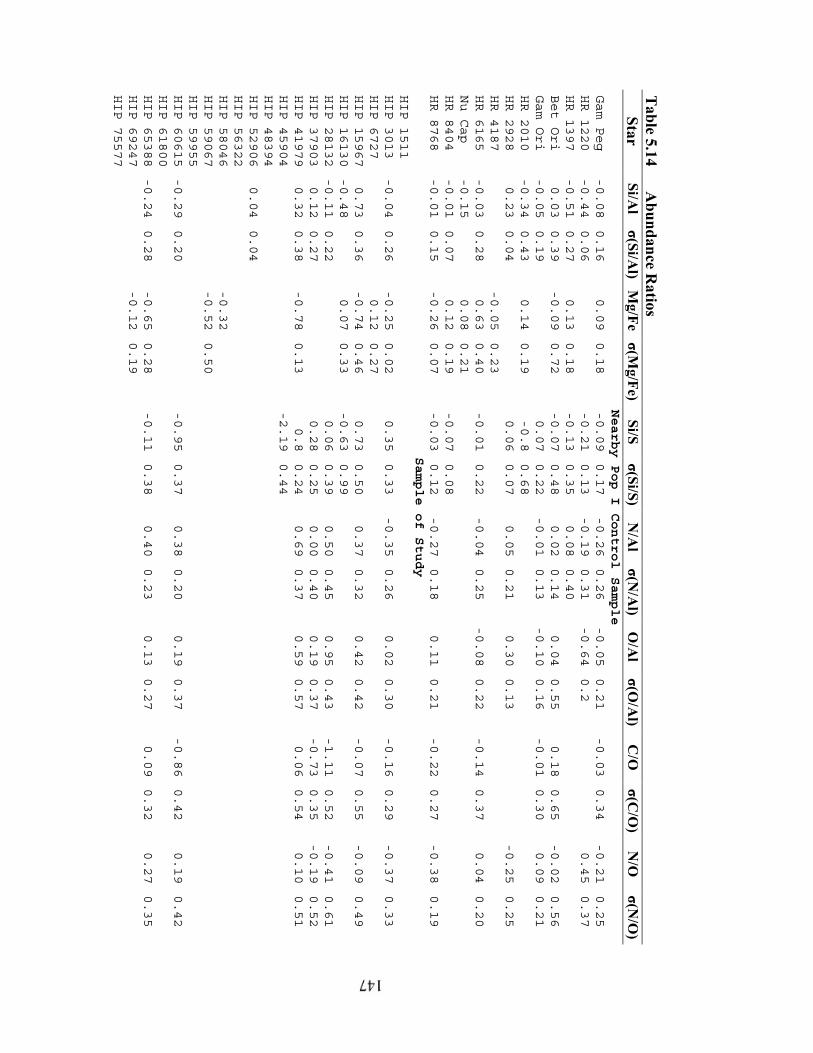
Table 5.14
Abundance R
atios Star
Si/Al
σ(Si/Al)
Mg/Fe
σ(Mg/Fe)
Si/S σ(Si/S)
N/A
l σ(N
/Al)
O/A
l σ(O
/Al)
C/O
σ(C
/O)
N/O
σ(N
/O)
Nearby
Pop
IControl
Sample
Gam
Peg
-0.08
0.16
0.09
0.18
-0.09
0.17
-0.26
0.26
-0.05
0.21
-0.03
0.34
-0.21
0.25
HR
1220
-0.44
0.06
-0.21
0.13
-0.19
0.31
-0.64
0.2
0.45
0.37
HR
1397
-0.51
0.27
0.13
0.18
-0.13
0.35
0.08
0.40
Bet
Ori
0.03
0.39
-0.09
0.72
-0.07
0.48
0.02
0.14
0.04
0.55
0.18
0.65
-0.02
0.56
Gam
Ori
-0.05
0.19
0.07
0.22
-0.01
0.13
-0.10
0.16
-0.01
0.30
0.09
0.21
HR
2010
-0.34
0.43
0.14
0.19
-0.8
0.68
HR
2928
0.23
0.04
0.06
0.07
0.05
0.21
0.30
0.13
-0.25
0.25
HR
4187
-0.05
0.23
HR
6165
-0.03
0.28
0.63
0.40
-0.01
0.22
-0.04
0.25
-0.08
0.22
-0.14
0.37
0.04
0.20
Nu
Cap
-0.15
0.08
0.21
HR
8404
-0.01
0.07
0.12
0.19
-0.07
0.08
HR
8768
-0.01
0.15
-0.26
0.07
-0.03
0.12
-0.27
0.18
0.11
0.21
-0.22
0.27
-0.38
0.19
Sample
of
Study
HIP
1511
HIP
3013
-0.04
0.26
-0.25
0.02
0.35
0.33
-0.35
0.26
0.02
0.30
-0.16
0.29
-0.37
0.33
HIP
6727
0.12
0.27
HIP
15967
0.73
0.36
-0.74
0.46
0.73
0.50
0.37
0.32
0.42
0.42
-0.07
0.55
-0.09
0.49
HIP
16130
-0.48
0.07
0.33
-0.63
0.99
HIP
28132
-0.11
0.22
0.06
0.39
0.50
0.45
0.95
0.43
-1.11
0.52
-0.41
0.61
HIP
37903
0.12
0.27
0.28
0.25
0.00
0.40
0.19
0.37
-0.73
0.35
-0.19
0.52
HIP
41979
0.32
0.38
-0.78
0.13
0.8
0.24
0.69
0.37
0.59
0.57
0.06
0.54
0.10
0.51
HIP
45904
-2.19
0.44
HIP
48394
HIP
52906
0.04
0.04
HIP
56322
HIP
58046
-0.32
HIP
59067
-0.52
0.50
HIP
59955
HIP
60615
-0.29
0.20
-0.95
0.37
0.38
0.20
0.19
0.37
-0.86
0.42
0.19
0.42
HIP
61800
HIP
65388
-0.24
0.28
-0.65
0.28
-0.11
0.38
0.40
0.23
0.13
0.27
0.09
0.32
0.27
0.35
HIP
69247
-0.12
0.19
HIP
75577

Table 5.14 (continued)
Star Si/A
l σ(Si/A
l) M
g/Feσ(M
g/Fe)Si/S
σ(Si/S)N
/Al
σ(N/A
l) O
/Alσ(O
/Al)
C/O
σ(C
/O)
N/O
σ(N
/O)
HIP
76161
0.07
0.21
0.00
0.36
0.31
0.31
-0.31
0.38
HIP
77131
-0.01
0.46
HIP
77716
0.73
0.25
0.25
0.23
0.52
0.30
0.64
0.39
0.33
0.44
-0.12
0.36
HIP
79649
-0.31
0.06
-0.74
0.08
-0.24
0.14
0.11
0.48
0.14
0.48
-0.35
0.50
HIP
81153
-0.21
0.15
0.16
0.19
-0.44
0.33
-0.5
0.26
-0.26
0.28
0.06
0.37
HIP
96130
-0.16
0.09
-0.21
0.09
HIP
98136
-0.07
0.36
-0.01
HIP
107027
0.08
0.15
-0.15
HIP
109051
-0.61
0.16
-0.24
HIP
112790
HIP
114569
-0.77
0.23
HIP
115729
-0.03
0.24
0.06
0.25
0.09
0.27
-0.27
0.34
-0.03
0.23
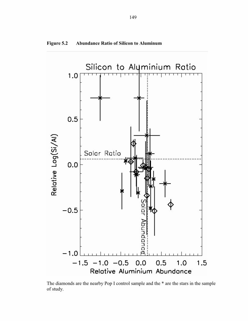
149
Figure 5.2 Abundance Ratio of Silicon to Aluminum
The diamonds are the nearby Pop I control sample and the * are the stars in the sample of study.

150
Figure 5.3 Abundance Ratio of Magnesium to Iron
The diamonds are the nearby Pop I control sample and the * are the stars in the sample of study.

151
Figure 5.4 Abundance Ratio of Silicon to Sulfur
The diamonds are the nearby Pop I control sample and the * are the stars in the sample of study.

152
The Si/Al, Mg/Fe, and Si/S ratios for the stars HIP 15967, HIP 41979, HIP
60615, and HIP 77716 consistently fall outside the range of values defined by the
nearby Pop I B star control sample. HIP 77716 has been classified as a PPN and
previous studies have found that it has a pattern of atmospheric abundances which is
indicative of an initial composition consistent with a metal poor halo star and
abundances lowered by dust formation (Napiwotzki, Heber, & Köpen 1994;
Napiwotzki, Herrmann, & Herber 2001)(See Section 7.3.1).
The N/O, C/O, N/Al, and O/Al ratios are used to identify enhancements that
could be due to mixing of processed material into a star’s atmosphere (Figures 5.5 - 5.8,
Table 5.14). The N/O values for the sample of study are not significantly different from
the distribution of values in the nearby Pop I control sample. The low C/O ratios of HIP
28132, HIP 37903, and HIP 60615 might be indicative of carbon depletion which is
common in hot PAGB stars (Parthasarathy et al. 2001). Six stars (HIP 15967, HIP
28132, HIP 41979, HIP 60615, HIP 65388, and HIP 77716) have elevated N/Al ratios
compared to the control sample and three of those (HIP 77716, HIP 28132, and HIP
41979) also have elevated O/Al ratios compared to the control sample.
HIP 15967, HIP 41979, HIP 60615, and HIP 77716 stand out with ratios which
could have been affected by dust grain formation or initial composition and also show
evidence of enhancement by nuclear processing. These stars, which have abundance
ratios that are persistently different from the stars in the nearby Pop I control sample,
are the best candidates to be old low mass evolved stars.

153
Figure 5.5 Abundance Ratio of Nitrogen to Oxygen
The diamonds are the nearby Pop I control sample and the * are the stars in the sample of study.
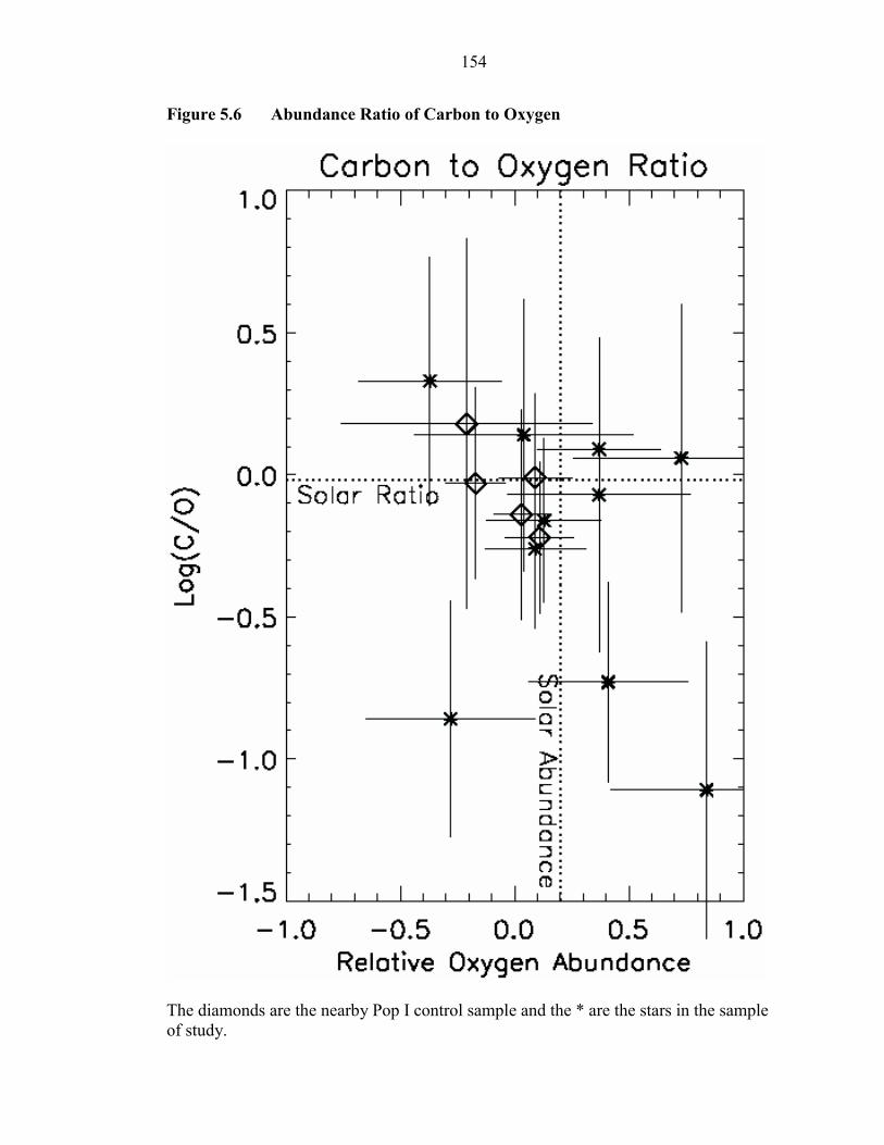
154
Figure 5.6 Abundance Ratio of Carbon to Oxygen
The diamonds are the nearby Pop I control sample and the * are the stars in the sample of study.

155
Figure 5.7 Abundance Ratio of Nitrogen to Aluminum
The diamonds are the nearby Pop I control sample and the * are the stars in the sample of study.

156
Figure 5.8 Abundance Ratio of Oxygen to Aluminum
The diamonds are the nearby Pop I control sample and the * are the stars in the sample of study.

157
5.5 Line Profile Fitting with MOOG
MOOG was used to interactively determine the rotational broadening (vsin (i))
and the abundances of the Mg II 4481 Å and C II 4267 Å features from synthesized
profiles. Vsin(i) was determined for each star by synthesizing a piece of spectrum using
several different broadening parameters and visually picking the one that fit best. The
piece of spectrum used to determine vsin(i) was either the Si III 4550 Å triplet or
another piece of spectrum containing at least one prominent unblended absorption line
(see Figure 5.9). The rotationally broadened profiles were calculated by the method of
Gray (1976). The best fit vsin(i) values are in Table 5.15. Figure 5.10 shows good
agreement between the vsin(i)’s measured and those published in the Yale Bright Star
Catalog (Hoffleit 1982) for the stars in the nearby Pop I control sample.
Figure 5.9 Example of Vsin(i) Fitting
This is a plot of the Si III 4567 line in the spectrum of Gam Ori with three synthetic fluxes plotted for comparison. From narrowest to widest, the profiles were generated using vsin(i) values of: 35 km/s, 50 km/s, and 65 km/s. The 50 km/s profile is the best fit.

158
Table 5.15 Vsin(i) Values and LTE Abundances from CII 4267 & Mg II 4481
Star
Teff (K)
vsin(i)(km/s)
C II 4267log ε(C)
Other log ε(C)
4267 EW((((maaaa)
Mg II 4481 log ε(Mg)
Other log ε(Mg)
Nearby Pop I Control SampleGamPeg 21750 4.0 7.53 8.13 220.0 7.31 7.53HR1220 28750 130.0 7.75 136.7 7.49HR1397 14250 20.0 8.32 8.72 112.3 7.56 7.29BetOri 18000 36.0 7.25 8.09 159.3 8.71 7.53GamOri 21750 50.0 7.72 8.25 254.5 7.20HR2010 10750 30.0 8.73 22.6 8.25 7.57HR2928 23750 20.0 7.25 167.7 7.13HR4187 10250 20.0 8.21 10.6 7.52 7.54HR6165 30000 8.0 7.65 8.11 96.0 7.64 8.19NuCap 10250 25.0 8.74 23.9 7.58 7.55HR8404 10250 2.0 7.81 14.5 7.85 7.49HR8768 17750 6.0 7.94 8.27 216.0 7.31 7.34
BHB Control SampleHD60778 8750 10.0 6.35 6.66HD74721 8750 3.0 6.63 6.57
PAGB Control SampleHD18100 27000 220.0 6.60 51.0 6.68HD44179 8250 20.0HD105262 9000 6.0 6.05HD119608 26500 50.0
Sample of StudyHIP 1214 11500 130.0 7.09HIP 1511 9000 20.0 7.53 2.0 5.69HIP 3013 19750 10.0 7.67 8.26 239.1 6.88 7.38HIP 6727 10000 6.00 8.10 7.26HIP 11809 13250 240.0 6.27HIP 11844 11250 130.0 7.46HIP 12320 13500 225.0 6.94 7.79HIP 15967 18500 15.0 7.83 8.50 260.4 7.47 7.87HIP 16130 13500 60.0 8.83 109.9 7.43 7.38HIP 28132 17000 100.0 7.36 7.87 141.8 6.34HIP 37903 18000 150.0 7.19 7.85 253.7 6.45HIP 41979 18000 8.0 9.73 8.95 391.3 8.24 7.38HIP 45904 21250 225.0 6.74 114.8HIP 48394 20250 225.0 6.59 93.1HIP 52906 18500 160.0 7.02 151.7 6.44HIP 55461 15500 140.0 7.14 137.9 7.04HIP 56322 26000 160.0HIP 58046 13250 230.0 7.48 35.3 7.30 7.04HIP 59067 15000 70.0 7.88 7.88 156.1 6.77 7.08HIP 59955 13500 225.0 6.92HIP 60615 22000 60.0 7.05HIP 61800 12500 150.0HIP 63591 10000 200.0 8.13 17.6 7.59HIP 65388 20000 5.0 8.26 8.71 366.5 7.62 7.45HIP 66291 17500 120.0 8.03 157.6 7.10HIP 69247 11250 20.0 6.28 10.0 7.26 6.68HIP 75577 12250 20.0 7.83 4.47

159
Table 5.15 Vsin(i) Values and LTE Abundances from CII 4267 & Mg II 4481
Star
Teff (K)
vsin(i)(km/s)
C II 4267log ε(C)
Other log ε(C)
4267 EW((((maaaa)
Mg II 4481 log ε(Mg)
Other log ε(Mg)
HIP 77131 32000 250.0 8.51 169.6 7.36HIP 77716 21500 5.0 8.15 6.59HIP 79649 21000 90.0 7.50 8.44 209.8 6.92HIP 81153 30000 80.0 7.77 8.02 160.9 7.33HIP 96130 23000 60.0 7.53HIP 98136 23250 140.0 7.61 250.2 7.34HIP 107027 22000 150.0 7.66 245.0 7.41HIP 109051 21000 105.0 7.32 229.8 6.85HIP 111396 13750 35.0 6.45HIP 112790 15250 70.0 8.26 156.1 6.94 7.43HIP 114569 17750 70.0 7.90 246.0 6.92HIP 115729 17750 25.0 7.78 8.10 190.3 6.89HIP 116560 8250 6.0 5.89
Figure 5.10 Vsin(i) Comparison With Bright Star Catalog
Vsin(i) as determined in this study for stars in the nearby Pop I B star control sample versus the values published for those stars in the Yale Bright Star Catalog

160
5.5.1 C II 4267 Å
The C II 4267 Å feature was modeled using the atomic data in Table 5.16. This
feature is known to be an unreliable measure of absolute C II abundance (Kane,
McKeith, & Dufton 1980). However it is the only carbon feature that can be measured
with any reliability in many B stars with large rotational broadening. C II 4267 Å was
modeled with the hope that it could be calibrated as a measure of relative composition.
Table 5.16 LTE Atomic Data for C II 4267 Feature Species λλλλ0000====((((Å) Ei (eV) Log(gf) C II 4267.001 18.0458 +0.5630C II 4267.183 18.0460 +0.7160C II 4267.261 18.0460 +0.4160
Source: Wiese et al. (1966)
Unfortunately it does not appear possible to use the LTE abundance derived
from the C II 4267 Å feature as a relative measure of carbon abundance. In some
cases MOOG was unable to reproduce the observed profile. Table 5.15 lists the LTE
carbon abundance measured from the C II 4267 Å feature relative to the average
abundance measured from other carbon lines. It is strongly suspected that NLTE effects
(Sigut 1996) significantly influence the formation of this line.
Figure 5.11 illustrates that there is no trend in the relative abundance derived
from the C II 4267 Å feature with respect to Teff. HIP 41979 is the point that stands out
from the others. If that point is ignored then C II 4267 Å may be useable as a gross
measure of carbon abundance with an accuracy of about ±0.5 dex.

161
Figure 5.11 LTE CII Abundance from the 4267 Feature Versus Teff
The difference in LTE Carbon Abundance From the C II 4267 feature relative to the abundance from other C II Lines versus effective temperature.

162
Figure 5.12 Equivalent Width of the C II 4267 Feature Versus Effective Temperature
The diamonds are the stars in the nearby Pop I control sample and the crosses are the stars in the sample of study.
A plot of the equivalent width of the C II 4267 Å feature versus the effective
temperature of the star (Figure 5.12) shows that most of the stars in the sample of study
follow the trend set by the nearby Pop I control sample. HIP 41979 and HIP 65388
have equivalent widths that are much larger than expected for their temperature while
HIP 45904 and HIP 48394 have significantly smaller equivalent widths than expected
for their temperature. All of these stars have peculiar abundance ratios (section 5.4.2)
and/or infrared excesses (section 7.4) which indicate they may not be normal Population
I B stars. HD 18100 from the PAGB control sample also has a small equivalent width
for its effective temperature. It may be related to the hot PAGB stars with low carbon

163
abundances (Parthasarathy et al. 2001). This relationship between equivalent width and
effective temperature requires further study in order to determine if the C II 4267 Å
feature could be used as an indicator of gross carbon abundance or other peculiarities in
hot B stars even though it is difficult if not impossible to translate the equivalent width
into an abundance. The feature may prove to be especially useful since it is strong and
easily measurable in even those stars that have very large rotational broadening.
5.5.2 Mg II 4481 Å
The Mg II 4481 Å feature was modeled with the atomic data in Table 5.17. This is a
very prominent feature in late type B stars and it was hoped that it could be used to
measure magnesium abundance in stars with large rotational broadening. Unfortunately,
this feature also proved to be an unreliable indicator of abundance. The abundances
derived from Mg II 4481 Å measured relative to other Mg II lines are give in Table
5.15. Figure 5.13 shows a large spread in relative abundances and a trend with respect
to effective temperature which is stronger when the two low points around 18000 K are
ignored.
Table 5.17 LTE Atomic Data for Mg II 4481 Feature Species λλλλ0000====((((Å) Ei (eV) Log(gf) Mg II 4481.126 8.8637 +0.7300Mg II 4481.150 8.8637 -0.5700Mg II 4481.325 8.8638 +0.5750
Source: Biermann & Lubeck (1948)

164
Figure 5.13 LTE Magnesium Abundance from the Mg II 4481 Feature Versus Effective Temperature
The difference in LTE abundance of magnesium calculated from the Mg II 4481 feature relative to the abundance from other Mg II Lines as a plotted as a function of effective temperature
The Mg II 4481 Å feature is not a reliable measure of abundance because Mg II
is a minor species in even the coolest B stars, composing less than 2% of the population
at the level of maximum contribution. The population of a minor species is so sensitive
to temperature and pressure that those parameters drive the calculation more than the
chemical composition (see section 5.6). In addition to being a minor species, the core
of this feature easily saturates making it sensitive to thermal velocity and
microturbulence. Mihalas (1972) demonstrated that there are also significant NLTE

165
effects at work in the transitions. As a result the feature is too sensitive to the
atmospheric model to measure abundance reliability.
The trend with respect to temperature is the result of the level of maximum
contribution being pushed higher in the model atmosphere with hotter effective
temperature (i.e. the temperature of the level of maximum contribution remains roughly
constant). Mg II 4481 Å may work well in B stars to detect a metallicity difference of
1.0 dex. However, it is not well suited for more sensitive measurements.
5.6 Contribution of Other Factors
5.6.1 NLTE Effects
NLTE effects, which are normally characterized as atomic level population
perturbations relative to LTE, influence both individual line formation and the overall
structure of a stellar atmosphere. These effects are more significant for some lines than
others. Kilian (1994) found that at the ±(0.1 to 0.2) dex level there is no difference in
abundances calculated using LTE assumptions versus NLTE calculations. The largest
departures from LTE values occur in stars with the highest effective temperatures.
Kilian (1994) speculated that NLTE effects may be partially or wholly “absorbed” by
the increased microturbulence values in LTE analyses.
NLTE effects may also impact the photometric effective temperature and
surface gravity relations since most of them rely on theoretical colors calculated from
stellar atmospheres that assume LTE. The role of NLTE effects with respect to these
calibrations is more significant in hotter (>20000 K) and lower gravity stars. Kilian et
al. (1991a) demonstrated that temperature estimates for B-stars made from the

166
Strömgren [c1] index are systematically 2000 K cooler than temperature estimates made
from H I and Si III lines after accounting for NLTE effects. Vrancken, Butler, & Becker
(1996) found that Kilian et al. (1991a) had overestimated this difference by at least 300
K to 500 K. Sigut (1996) found no similar offset between NLTE temperature estimates
and the Napiwotzki et al. (1993) [u-b] temperature relation. The exact effect of NLTE
on derived stellar parameters is an unresolved subject of ongoing study. The best
course of action is to be conscious of the fact that, particularly in hot supergiants, there
may be a tendency to overestimate the stellar effective temperature.
5.6.2 Temperature and Gravity Effects
Uncertainty in the parameters that define the models translates directly into
uncertainty in the abundances. Each atomic species is affected differently by these
uncertainties. Minor species, being very sensitive to temperature and pressure, are most
affected by perturbations in the structure of the models. These effects can be quantified
by comparing the relative abundances calculated from the same equivalent widths using
different models.
The effect of model choice on the derived abundances was quantified using
three stars selected from the nearby Pop I control sample in the hot (HR 6165, Teff=
30000, log(g) = 3.75, ξt= 7 km/s), middle ( HR 8768, Teff= 17750, log(g) = 3.75, ξt= 8
km/s), and cool (Nu Cap, Teff= 10000 K, log(g) = 4.25, ξt= 2.5 km/s) temperature
ranges. LINES synthesized equivalent widths at solar abundances for absorption
features identified in these stars. The synthesized equivalent widths were used to
calculate the relative abundances in models within ±0.25 dex in log(g) and ±5% in

167
effective temperature. These surface gravity and effective temperate ranges roughly
correspond to the level of confidence placed in the determination of these parameters
for stars in the sample. The resulting differences in abundance with respect to
atmospheric model are given in Table 5.18.
In all cases the minor species (representing less than 5% of the population at the
level of maximum contribution) show the largest variation with respect to the
temperature and gravity of the selected model. On a fairly consistent basis, the
calculated offsets are well within the typical standard deviation of the abundances
calculated from the measured equivalent widths. This analysis also identifies some
species that are very stable with respect to temperature and gravity. In the hottest stars,
Ne II appears to be very reliable. In the stars in the mid-temperature range S II is very
consistent. And in the coolest stars, Mg II (excluding Mg II 4481 Å) and Fe II produce
dependable results that are only marginally affected by the model parameters.
Iron, aluminum, oxygen, and sulfur are of special interest since they are used as
referents to measure abundance ratios (Section 5.4.2). In the cool B stars, Fe II is very
stable with respect to changes in temperature and pressure but becomes less stable in the
mid-range of temperatures. In hot B stars, the Fe III abundance is almost as stable as Fe
II is in the mid-range but not as stable as Fe II in the cool range. Al III appears to be as
stable as the iron species used in the mid and high temperature ranges. Oxygen,
measured from O II, is most reliable in the high temperature range but more susceptible
to perturbations in the mid-range. S II is the most reliable element in the mid-range but
is more unstable in the low range. S III only accounts for 5% to 10% of the population

168
Table 5.18 Abundance Changes as an Effect of Model Choice
HR 6165
Log(g) 3.50 3.75 4.00
31500 0.25 0.35 -0.03 0.20 0.07 0.100.43 0.70 0.19 0.35 0.05 0.140.33 0.58 0.14 0.31 0.03 0.150.20 0.48 0.07 0.24 0.01 0.10
30000 0.20 0.13 C II Al III -0.11 -0.09
Teff 0.16 0.23 N II Si III -0.10 -0.13
0.14 0.19 O II S III -0.08 -0.100.07 0.17 Ne II Fe III -0.01 -0.10
28500 -0.07 -0.09 -0.19 -0.20 -0.26 -0.26-0.08 -0.12 -0.19 -0.26 -0.26 -0.33-0.06 -0.13 -0.15 -0.23 -0.18 -0.260.01 -0.09 0.01 -0.21 0.06 -0.27
HR 8768 Log(g)
3.50 3.75 4.0018750 -0.17 -0.30 -0.12 -0.19 -0.06 -0.07
-0.35 -0.40 -0.22 -0.26 -0.08 -0.11-0.47 0.05 -0.30 0.04 -0.13 0.05
0.29 0.24 0.2117750 -0.06 -0.13 C II Al III 0.08 0.13
Teff -0.14 -0.15 N II Si III 0.14 0.14
-0.17 -0.02 O II SII 0.16 0.030.04 Fe II -0.03
16750 0.08 0.09 0.16 0.22 0.25 0.360.11 0.13 0.26 0.28 0.40 0.420.16 -0.04 0.33 0.01 0.49 0.06
-0.22 -0.25 -0.27
Nu Cap Log(g)
4.00 4.25 4.5010750 -0.04 0.14 -0.02 0.19 0.01 0.25
-0.50 0.66 -0.38 0.59 -0.25 0.520.42 0.09 0.43 0.16 0.43 0.23
Teff 10250 -0.03 -0.05 Mg II Cr II 0.03 0.05
-0.13 0.08 S II Fe I 0.14 -0.08-0.02 -0.06 Ti II Fe II 0.02 0.06
9750 -0.01 -0.17 0.02 -0.13 0.05 -0.080.11 -0.28 0.26 -0.35 0.39 -0.43
-0.25 -0.17 -0.22 -0.12 -0.19 -0.08
* The center box in each chart lists the elements tested. The other boxes list the differential abundance with respect to the center grid point for each element in the same order they are listed in the center box.

169
in the high range making it more sensitive to changes in temperature than pressure
structure in the hottest B stars.
5.6.3 Microturbulence: Effect on Equivalent Widths
Microturbulence affects the abundances in two ways:
1. It affects abundances calculated from equivalent widths through line broadening
and
2. It influences the pressure structure of the model atmosphere directly.
In this subsection the former will be discussed. The latter will be explored in the next
subsection.
The effects of microturbulent broadening on abundances calculated from
equivalent widths was explored using synthesized equivalent widths from the same
three stars used in the previous subsection (HR 6165, HR 8768, and Nu Cap). Figures
5.14 to 5.16 illustrate how the relative abundance calculated from the synthetic
equivalent widths change as the model is held constant and ξt is varied. The species
which show the largest variation are often the heavier nuclei because they have lower
thermal velocities which can be dominated by microturbulence. Normally the
microturbulent velocity can be set with an accuracy of at least ±2 km/s but this
uncertainty may be higher for stars using a “borrowed” ξt (see section 5.3).

Figure 5.14 E
ffect of Microturbulence on A
bundances in Nu C
ap
The curves show
the relative change in abundance measured in a star w
ith the parameters (T
eff = 10000 K, log(g) = 4.25 dex, ξ
t = 2.5 km
/s) for an element from
a given species as the microturbulence is changed in the dam
ping parameter. In the left panel the dotted
line is Mg II, the dashed line is S II, and the dash-dot line is Ti II. In the right panel the dotted line is C
r II, the dashed line is Fe I, and the dash-dot line is Fe II.

Figure 5.15 E
ffect of Microturbulence on A
bundances in HR
8768
The curves show
the relative change in abundance measured in a star w
ith the parameters (Teff= 17750 K
, log(g)= 3.75 dex, ξt = 8.0
km/s) for an elem
ent from a given species as the m
icroturbulence is changed in the damping param
eter. In the left panel the dotted line is N
II, the dashed line is O II, and the dash-dot line is A
l III. In the right panel the dotted line is Si III, the dashed line is S II, and the dash-dot line is Fe II.

Figure 5.16 E
ffect of Microturbulence on A
bundances in HR
6165
The curves show
the relative change in abundance measured in a star w
ith the parameters (Teff= 30000 K
, log(g)= 3.75 dex, ξt = 7.0
km/s) for an elem
ent from a given species as the m
icroturbulence is changed in the damping param
eter. In the left panel the dotted line is C
II, the dashed line is O II, and the dash-dot line is A
l III. In the right panel the dotted line is Si III, the dashed line is S III, and the dash-dot line is Fe III.
173
5.6.4 Microturbulence: Effect on Structure of the Models
A change in microturbulence has no significant effect on the temperature
structure of the model atmosphere but it can perturb the pressure structure by as much
as 20% at an optical depth of one. In order to quantify the effect such a change in
pressure structure could have on the derived abundances, the results from the models in
the atmosphere grid were compared to results from a series of model atmospheres
which were calculated using the parameters of HR 6165, HR 8768, and Nu Cap with
different microturbulent velocities. Models were produced in each temperature range
with ξt= 0 km/s. Similar models were calculated for HR 6151 and HR 8678 using ξt= 8
km/s. A model with higher ξt for Nu Cap was not produced because a microturbulent
velocity that is much higher than the thermal velocity causes models on the cool end of
the temperature range to become unstable and not converge. The model atmospheres
with different microturbulent velocities were used to convert the synthetic equivalent
widths (described in the previous two subsections) to abundances and measure the
abundance difference caused by a significant change in ξt as an input to ATLAS9. The
results in Table 5.19 show that the changes in the pressure structure caused by variation
in microturbulence have no significant effect on the abundances.

174
Table 5.19 Effect of ξt in Models on Abundances HR 6165
ξt (km/s) C II N II O II Ne II Al III Si III S III Fe III 0 -0.02 -0.01 -0.03 -0.01 -0.02 -0.05 -0.04 -0.018 0.03 0.04 0.01 0.00 0.02 0.02 0.02 0.04
HR 8768 ξt (km/s) C II N II O II Al III Si III S II Fe II
0 0.01 0.01 0.01 0.01 0.01 0.00 0.008 -0.05 -0.09 -0.12 -0.08 -0.10 0.00 0.06
Nu Capξt (km/s) Mg II S II Ti II Cr II Fe I Fe II
0 0.01 0.02 0.00 0.01 -0.02 0.01
5.6.5 Stellar Rotation: Effects on Structure of the Models
Rotational broadening does not enter into the damping parameter so it has no
significant effect on the equivalent widths of individual lines. However, rapid rotation
distorts a star and causes variation of the effective temperature and gravity over the
surface. If the photospheric parameters vary over the stellar surface then changes in the
temperature and pressure structure of the atmosphere will have an impact the equivalent
widths. Eight (8) of the stars in the sample of study have measured vsin(i) in excess of
200 km/s, with the fastest being 260 km/s. It is important to note that a low vsin(i) does
not necessarily mean that the star is not a rapid rotator since any star viewed from a
high inclination angle or pole-on will have small vsin(i).
Collins, Truax, & Cranmer (1991) produced theoretical models and profiles of
hydrogen lines, helium lines, and the Mg II 4481 Å feature in rotating B stars. All the
spectral features simulated in the Collins et al. (1991) study are more sensitive to
changes in temperature and pressure structure of the atmosphere than most metallic
175
lines. As a result, the differences that they calculated are interpreted as an upper limit
on the effect rotation may have on the equivalent widths of weaker metal lines.
Collins et al. (1991) showed a less than 5% difference between equivalent
widths of the lines they simulated in stars with no rotation and stars rotating at critical
velocity viewed pole on. This means that there is little concern about potential errors
in the abundances calculated from equivalent widths in a narrow lined star regardless of
its true rotational speed. The predicted equivalent widths increased by less than 10% in
stars rotating at 80% of the critical velocity viewed from a lower inclination. An
increased equivalent width would lead to an overestimated abundance. For the Si III
4552 Å line, which is strong and typical of measurable lines in hot stars with large
rotational broadening, a ten percent change in equivalent width corresponds to a
difference in abundance of 0.11 dex at Teff= 20000 K and 0.09 dex at Teff = 30000 K
under the assumptions and models used in this analysis. In the most extreme case, the
over estimation of the abundance is of about the same size as other effects on
temperature and pressure structure of the atmosphere. Since the critical rotation
velocity for most B stars is on the order of 300 km/s to 400 km/s or more, rotation
should have little effect on the abundances derived from the equivalent widths of the
stars in this study.