chapter 5 measuring carbon in shrubs - nitc - north · pdf file ·...

Chapter 5 Measuring Carbon in Shrubs

David C. Chojnacky and Mikaila Milton

Abstract Although shrubs are a small component of the overall carbon budget, shrub lands and shrub cover within forested lands warrant monitoring with consistent procedures to account for carbon in shrubs and to track carbon accumulation as communities change from shrubs to trees and vice versa. Many different procedures have been used to sample and measure shrubs (Bonham 1989) but only three types are selected here, to represent a range from simple and subjective to more time-con- surning but objective measurements. Although the goal is to measure shrub carbon, the methods outlined here estimate biomass-which is about 50% carbon. For sample design, we advocate compatibility with the USDA, Forest Service, Forest Inventory and Analysis (FIA) program by using transects, microplots, or quadrats arranged w i t h or near FIA subplots. Three basic methods are suggested for measuring shrub biomass: (1) cover estimations along transects, including point-intercept and line- intercept; (2) visual cover estimates in fixed area units; and (3) diameter measurement within fixed-area sampling frames. The 3rd method for measurement of individual shrub stem-diameters provides the most robust data for estimating biomass (and by extension, carbon) but requires the most field time. The other two methods allow more rapid measurements of shrub cover along transects or within plots. Our summary provides a framework for collecting shrub measurements three different ways; however, more work will likely be needed to develop appropriate equations that equate cover or stem measurements with biomass for various species.

Keywords Cover measurement, diameter measurement, microplot, shrub, transect sampling

D.C. Chojnacky US Forest Service Washington, DC, Current address: Virginia Tech Department of Forestry, 144 Rees Place, Falls Church, VA 22046 E-mail: [email protected]

M. Milton National Science Foundation, Arlington, VA, Current address: National Park Service, 1900 Anacostia Drive SE, Washington, DC 20020 E-mail: mikaila-milton @ nps.gov

C.M. Hoover (ed.) Field Measurements for Forest Carbon Monitoring, O Springer Science+Business Media B.V. 2008

D.C. Chojnacky, M. Milton

5.1 Introduction

The movement of carbon in its many forms - between the living and nonliving forms of the biosphere, atmosphere, oceans, and geosphere - is widely recogniz- able as the carbon cycle. With the amount of carbon in the atmosphere escalating at a rapid rate today, management focus is increasingly turning to the sequestration of more carbon where possible. In forests, shrubs are a small component of the overall carbon budget, estimated as 2% of total forest carbon (Kimble et al. 2002). However, shrubs often dominate early successional stages of many forest types, particularly following fires, and in some cases vigorous shrub communities constitute a primary land management objective for wildlife cover and for- age. Furthermore, shrub and other understory growth (net primary production) can be comparable to that of trees (Nilsson and Wardle 2005) and constitutes a major source of carbon for the forest floor and soil. Therefore, shrubs may not sequester much carbon on land but they may be very important for adding to the soil carbon pool.

Consequently, from a carbon stock perspective, shrub lands and shrub cover within forested lands warrant monitoring with consistent procedures to account for carbon in shrubs and to track carbon accumulation as communities change from shrubs to trees and vice versa.

Procedures to measure forest vegetation differ depending on the life forms of live and dead vegetation. Typically, either fixed-area plots or transects are used to sample vegetation material; estimates generally are expressed in tons or Mg per unit area. Shrubs have been successfully sampled with both plots and transects (Peet et al. 1998, Korb et al. 2003, McMillin and Allen 2003).

SmpW me*& ifcm.Eium - lke a d to smey &e &s~b&oa of @@dsmns %mss a &VCR

m&, rzsiag m p l e p&& &oag &e Zim tct CO!I& && &%t em be 8sed ta d e e b e &e whoEe ppa1agaa area,

#tt% - plot (e%ak, warn, or ) of a Exed size ased to swey a wfiaa of a f~~hest 01: other s e a tca wllm $a& &at em k u d to d e s & k &e wkoIe ppulagoa area.

Elsewhere in this book, procedures developed by the USDA, Forest Service, Forest Inventory and Analysis (FIA) program (FIA 2005) are recommended for measuring carbon in forest trees. However, the FIA shrub measurements were not designed for measuring carbon. Therefore, in this chapter we recommend shrub measurement procedures that are compatible as an add-on to the FIA protocol and are more suited to the measurement of shrub carbon.

Many different procedures have been used to sample and measure shrubs (Bonham 1989) but only three types are selected here, to represent a range from simple and subjective to more time-consuming but objective measurements. These methods incorporate two different sample-design philosophies: transects and fixed-area

5 Measuring Carbon in Shrubs 47

%B&g shrubs A s b b is a woody plane that generally has mdufeipfe s&ms @owing from rfie w e root system, The w d y g ~ w t h f o m distkg~plishes a shrub from n o n - w d y herbxmclrus plmts. Wowever, it is sometimes &fic.uXt to distinguish shrubs fm @ms based on grow& fom, so it is rnsuzilly necessafy to consult f o m d s p i e s lists, such as the comprehensive Xist of U.S. trees compiled by the R A (FIA ZWa). The F U list is a g a d stming point for deciding whether a woody p h t is a &m caf $bmb far eilch projwt, Meverphebss, a few w d y species that R A eaDs ;a 'kee" mi&t be: btte:r m e ~ u r d as a "'skW' sereh a some s p i e s of Amkmhiar, Prt(p9.%rs, anand Sala'x. merefare, shrub degnidons far indivi&tnal projects should be: es&b Iished at the outset of any monitoring progmm. ln aaition to chossing which species are deflrrmd as s h b s , it will be practical to set a lower basd &meter limit below which individrnds me conside~d go be "he&amous'* fix meas- wement prnpses. These smdl-diameter plants ase: often more eEciently measwed with the he&ac:eo?~~s layer (wgch iz; not cover& in this chapter).

plots. Generalized equipment lists, procedures, calculations, and discussion are provided for comparison purposes. References are provided for details on imple- mentation of various methods.

Although the objective is to measure shrub carbon, none of the methods outlined here estimates carbon directly. Instead, either shrub cover or basal area is measured in the field, and biomass-which is about 50% carbon (Kort and Turnock 2003)-is estimated from regression subsampling (Lohr 1999) or from auxiliary models. We provide an overview of some existing auxiliary models for estimating shrub biomass and show how the model equations were applied during a 2004 test within piedmont hardwood forests in the eastern United States.

48 D.C. Chojnacky, M. Milton

5.2 Incorporating Shrub Measurements into the FIA Design

FIA procedures have become the standard for strategic-scale sampling of forests in the United States. FIA has more than 70 years of experience monitoring wildland and managed forests and more than 10 years of experience monitoring forest health indicators, which include shrub cover measurements. The FIA program already covers all forest lands in the US with a grid of 120,000 plots and is currently adapt- ing its forestland procedures for use in urban forest health monitoring efforts.

The FIA design includes fixed-plot procedures for measurement of understory vegetation diversity and structure, including shrub species (FIA 2002). Shrubs are measured as cover in a nested design as part of the phase 3 (P3) or Forest Health Monitoring (FHM) protocol. In FHM plots, cover is visually estimated over each subplot as well as in three 1 m' quadrats within each subplot. In the subplots, cover is recorded in classes (1-5%, 6-lo%, 11-20%, 2140%, 41-60%, 61-80%, and 81-100%) for all species including shrubs. In the quadrats, cover is estimated to the nearest 1% for each species.

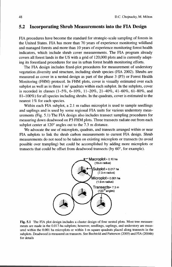
Within each FIA subplot, a 2.1 m radius microplot is used to sample seedlings and saplings and is used by some regional FIA units for various understory measurements (Fig. 5.1) The FIA design also includes transect sampling procedures for measuring down deadwood on P3 FHM plots. Three transects radiate out from each subplot center at 120' angles out to the 7.3 m distance.

We advocate the use of microplots, quadrats, and transects arranged within or near FIA subplots to link the shrub carbon measurements to current FIA design. Shrub measurements do not need to be taken on existing microplots or transects (to avoid possible over trampling) but could be accomplished by adding more rnicroplots or transects that could be offset from deadwood transects (by 60°, for example).

t...' Macroplot= 0.10 ha (18-rn radius)

Fig. 5.1 The FIA plot design includes a cluster design of four nested plots. Most tree measurements are made in the 0.017-ha subplots; however, seedlings, saplings, and understory are measured within the 0.001 ha microplots or within 1-m square quadrats placed along transects in the subplots. Deadwood is measured on transects. See Bechtold and Patterson (2005) and FIA (2004b) for details


Although it is common to sample vegetation composition and structure at different scales (Peet et al. 1998), such methods were designed to capture community structure and to track rare and alien species rather than to provide an objective measure for shrub carbon. Furthermore, methods using variable-size sampling frames for different vegetation structures have not been widely adapted for biomass or carbon estimation.

Therefore, each shrub measurement method described in this chapter uses a single-size sample frame for each plot. However, the various methods presented still offer flexibility for measuring different plant communities. Our assumption is that the primary objective is to achieve an unbiased estimate of total shrub carbon, rather than to monitor community composition over time or to sample all plant species for the purpose of detecting rare plants or invasive species.

5.3 Shrub Sampling Methods

We focus on field estimation of shrub cover (or a cover surrogate) and on measurement of basal diameters (basal area) to provide the data for estimating biomass through the use of regression subsampling (Lohr 1999, p. 74) or auxiliary models. Carbon in shrubs is assumed to constitute about 50% of biomass (Kort and Turnock 2003). Cover is defined as the vertical projection of vegetation from the ground as viewed from above (Elzinga et al. 1998). Shrub measurements are presented in the context of sampling points along a transect or fixed-area sampling units, as part of a larger survey where plots constitute sample units that are aggregated in classical sample designs for estimating population attributes (Cochran 1977). The objective of these shrub sampling techniques is to adequately sample a plot for shrub cover or basal area. In terms of overall sample design, these plots can be viewed as measuring cover or basal area in a "support region" around a point, which is designed to be large enough to capture the variation at that point and represent a true estimate of the parameters measured (Chojnacky 1998, p. 3). The shrub data collected as part of the plot measurement protocol can then be combined with other carbon components sampled around the same point without necessarily using exactly the same area dimensions for each element of the vegetation.

Plot dimensions in typical vegetation studies (such as those conducted by FIA) have several sample size features that are critical to the performance of each of sample method; those features include transect length, plot or quadrat size, and number of sample measurements. However, no attempt is made in this chapter to establish optimum dimensions for each feature; rather, initial recommendations are given based on a field test conducted in eastern deciduous forests in 2004 (described later in this chapter). To fully optimize application of the procedures presented here, additional field testing is suggested for each major ecosystem or area of the US.

Three basic methods are suggested for measuring shrub biomass: (1) cover estimations along transects, including point-intercept and line-intercept; (2) visual cover estimates in fixed area units; and (3) diameter measurement within fixed-area sampling frames. Choice of method to use depends on a project's objectives, available


staff time, funds available, level of precision and degree of confidence desired, type of vegetation being sampled, season, and other site-specific factors. Regardless of method, it is best to sample during the period of peak foliage development to ensure consistency among samples and to avoid complicated adjustments that otherwise would be needed to account for seasonal leaf conditions.

5.3.1 Transect Intercept Cover Sampling

Transect sampling - collecting data at defined points along a line -provides a relatively simple way to measure cover objectively. We present two different ways to measure shrub cover along a transect: point-intercept and line-intercept.

5.3.1.1 Point-Intercept Cover

The point-intercept method records shrub vegetation that intercepts or "hits" a pole perpendicular to a transect at specified sampling intervals (for example, hits along a 2 m pole placed at 1 m intervals) (Fig. 5.2). The optimal point-sampling interval and numbers of transects needed would depend upon vegetation density, and would be best determined by pilot testing. Hits at a given point can include only the uppermost layer or those in some specific layering scheme. To obtain the most flexible data for calculating cover layers or density measures, every vegetation hit can be recorded at each point.

Equipment

30 m tapes Pole (generally 2 m) marked in centimeter intervals Compass Chaining pins

hit miss hit hit

transect line

Fig. 5.2 The point-intercept method tallies vegetation hits touching a pole perpendicular to a transect at predetermined intervals


Procedure

Using 30 m tapes, establish transects that radiate from each FIA subplot center. Offset shrub-measurement transects from deadwood transects, to minimize site disturbance and trampling that would affect other protocol measurements. Use pins to secure tapes at each end of the transect to keep spacing between sample points accurate. There is probably no need to slope-correct transects (because cover is not related to a strict map-area-based sampling frame); however, if slope correction is desired, then the total length of the slope-corrected transect would be divided by the number of sample points to obtain a new distance between points.

At each sample point along the transect, record either the highest intersection of vegetation hitting the pole or the heights of the highest intersections within height classes, if cover at different heights or layers of vegetation is desired. To obtain the most flexible data for calculating cover layers or density measures, one could also record multiple vegetation hits at a given point. Vegetation hits can be recorded by species or species group, depending on the desired detail.

The vertical pole should be perpendicular to the transect tape; a plumb-line might be useful to ensure field crew consistency. A vegetation hit needs to be carefully defined to account for irregular leaf and branching shapes and leaf movement on windy or rainy days.

Calculations

Percent shrub cover for a plot is calculated from point-intercept sampling by sum- ming the number of sample points where vegetation intersects or hits the pole and dividing by the total number of points sampled. Cover can be calculated for each height layer if more than one layer is sampled.

N P,jk cover,, = 100 -

,=I N

where cover,, = percent shrub cover for height layer j of species or species group k

1 if foliage intercepts sample pole at point i for height layer j of species k 0 otherwise

N = total number of points sampled in layer j for all transects on plot

Note that one hit is generally used at each point (i) for any given cover or cover layer calculation. However, if more hits are recorded there is an opportunity to study the frequency of hits within height layers, which may be useful for constructing biomass equations from these data.

Biomass is calculated from equations using the calculated cover but these equations most likely will need to be developed. Measuring biomass for construc- tion of these equations (as described later) will be somewhat complicated because


two different sample frames will be needed since biomass cannot be estimated directly from transects. However, the point-intercept method has the flexibility of describing cover density in two dimensions (by using layers), which may prove quite useful in constructing generalized biomass equations for species groups.

Summary

This quantification of foliar frequency along transects provides an objective estimate of shrub cover at various layers for each species or species group. It is possible to use point-intercept sampling even in dense mixed-species communities where the foliage of many species overlaps. The point-intercept method is easy to imple- ment without intensive training of field personnel. Its limitations for use in biomass estimation include: the possibility of bias in pole-intercept measurement for recording "hits" and the lack of appropriate species-level equations for converting cover to biomass. But the method offers much potential for constructing new biomass equations because of its flexibility to objectively measure shrub cover hits by species at multiple layer heights (which would provide additional variables related to density of shrub branching patterns, which in turn may help with biomass prediction).

5.3.1.2 Line-Intercept Cover

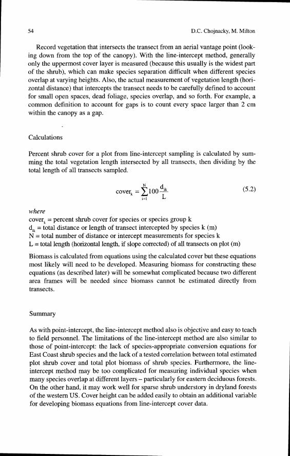
The line-intercept method records vegetation cover by measuring the length (horizontal distance) of shrub cover that intersects the transect (Fig. 5.3). Generally only the uppermost layer of cover is measured. The idea is to measure the extent of canopy that shades the ground when the sun is directly overhead.

Equipment

30 m tapes Pole (generally 2 m) marked in centimeter intervals Compass Chaining pins

Procedure

Using 30 m tapes, establish transects that radiate from each FIA subplot center. Offset shrub-measurement transects from deadwood transects, to minimize site disturbance and trampling that would affect other protocol measurements. Use pins to secure tapes at each end of the transect to keep spacing between sample points accurate. There is probably no need to slope-correct transects (because cover is not

5 Measuring Carbon in Shrubs

transect line

measure

measure

measure

measure

measure

measure this distance I

transect line

Fig. 5.3 Line-intercept methods measure the length of vegetation intersecting the transect on a horizontal plane

related to a strict map-area-based sampling frame); if slope correction is desired, then cover would be measured along the total length of the slope-corrected transect. However, calculations of slope-corrected transects would use horizontal transect length in the formula (which could result in more than 100% cover because a slope- corrected transect is longer than a horizontal transect).


Record vegetation that intersects the transect from an aerial vantage point (look- ing down from the top of the canopy). With the line-intercept method, generally only the uppermost cover layer is measured (because this usually is the widest part of the shrub), which can make species separation difficult when different species overlap at varying heights. Also, the actual measurement of vegetation length (horizontal distance) that intercepts the transect needs to be carefully defined to account for small open spaces, dead foliage, species overlap, and so forth. For example, a common definition to account for gaps is to count every space larger than 2 cm within the canopy as a gap.

Calculations

Percent shrub cover for a plot from line-intercept sampling is calculated by sum- ming the total vegetation length intersected by all transects, then dividing by the total length of all transects sampled.

dik cover, = 100 - ,=I L

where cover, = percent shrub cover for species or species group k d , = total distance or length of transect intercepted by species k (m) N = total number of distance or intercept measurements for species k L = total length (horizontal length, if slope corrected) of all transects on plot (m)

Biomass is calculated from equations using the calculated cover but these equations most likely will need to be developed. Measuring biomass for constructing these equations (as described later) will be somewhat complicated because two different area frames will be needed since biomass cannot be estimated directly from transects.

Summary

As with point-intercept, the line-intercept method also is objective and easy to teach to field personnel. The limitations of the line-intercept method are also similar to those of point-intercept: the lack of species-appropriate conversion equations for East Coast shrub species and the lack of a tested correlation between total estimated plot shrub cover and total plot biomass of shrub species. Furthermore, the line- intercept method may be too complicated for measuring individual species when many species overlap at different layers - particularly for eastern deciduous forests. On the other hand, it may work well for sparse shrub understory in dryland forests of the western US. Cover height can be added easily to obtain an additional variable for developing biomass equations from line-intercept cover data.


5.3.2 Visual Cover Sampling

Visual (or ocular) cover estimation within fixed-area plots is a relatively quick and popular way to estimate cover (Fig. 5.4). Cover can be visually estimated in units either to the nearest percent or within some predetermined cover classes (such as FIA's classes described earlier in this chapter). Although it is not possible to actually estimate cover to the nearest percent, recording the best estimate possible (to the nearest percent) is sometimes preferred over the use of cover classes when averaging many estimates. For one reason, large class boundaries may accentuate errors when dealing with border-line calls; furthermore, data collected in classes is problematic for averaging because the usual assumption of "class midpoint equal to class mean" can lead to bias when actual cover is not normally distributed within classes.

Two variations of this method are suggested that will fit within the FIA design: (a) cover estimates for microplots arranged within an FIA subplot or (b) cover for

Fig. 5.4 Visually estimating shrub cover is a simple and popular technique but requires careful attention for consistent application


small quadrats placed along transects within a subplot. By choosing either method, the FIA nested design is reduced to a single sampling frame, which is more consistent with our biomass objective.

5.3.2.1 Visual Cover for Microplots

The FIA design includes one 2.1 m radius microplot within each subplot, which is logical for sampling visual cover. However, the use of more microplots and different size radii might improve the estimate or sampling efficiency. We recommend that some pre-testing be conducted before deciding on the size and number of microplots needed.

Equipment

30 m tapes Compass Stakes or chaining pins Flagging Percentage-area guides for aiding visual estimation Pole (generally 2 m) marked in centimeter intervals

Procedure

Within each FIA subplot, locate and identify the microplot boundary with stakes or flagging. Estimate vegetation cover (of species or species group) from an aerial vantage point; if done by more than one person, average the estimates. For more repeatable and consistent estimation, it might be useful to divide the microplot into four quadrants; estimate the quadrants separately and then average the results. Estimation guides, such as pieces of cloth representing known quadrant areas, also are useful, at least for initial training. For example, each quadrant of a 2.1 m microplot would have square cloth guides with 59, 42, or 19 cm side dimensions to estimate lo%, 5%, or 1% of the quadrant area, respectively. Other estimation guides include pictures of microplots in shaded dot patterns representing percentages of cover for random and clumped arrangements for each quadrant. Cover height can also be measured with a pole, which provides an additional variable for cover-to- biomass modeling.

Calculations

No cover calculations (other than averages of all estimates within a plot) are needed because percent cover is estimated directly on the microplot or quadrant by species


or species group. Two or more crew members also could make independent estimates of the same spots for additional averaging. Biomass is calculated from equations using the estimated cover. Some cover-based equations exist but more likely will need to be developed. Measuring biomass for constructing these equations (as described later) will be straightforward because shrubs on the microplots or quadrants simply can be cut and weighed.

Summary

Visual estimation is a popular, quick, and easy way to estimate cover but it requires careful training and quality control to maintain consistency. Forestry has a rich history of many such ocular measurements that can be quite effective under the right circumstances. The primary limitation is the subjectivity of visual estimates (there is often a credibilitylobjectivity worry about "visual estimates" depending on the conscientiousness of field crews), as well as a lack of accurate cover-to-biomass equations. Therefore, careful comparison testing against a more objective method is suggested before selecting visual cover estimation on microplots. Also, some type of estimation aid as described above is highly recommended.

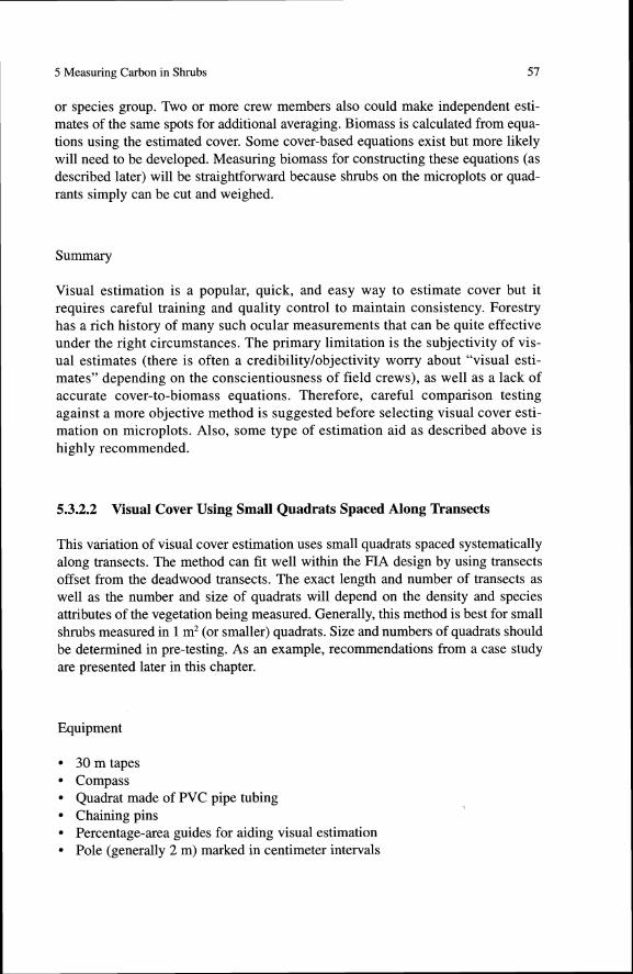
5.3.2.2 Visual Cover Using Small Quadrats Spaced Along Transects

This variation of visual cover estimation uses small quadrats spaced systematically along transects. The method can fit well within the FIA design by using transects offset from the deadwood transects. The exact length and number of transects as well as the number and size of quadrats will depend on the density and species attributes of the vegetation being measured. Generally, this method is best for small shrubs measured in 1 m2 (or smaller) quadrats. Size and numbers of quadrats should be determined in pre-testing. As an example, recommendations from a case study are presented later in this chapter.

Equipment

30 m tapes Compass Quadrat made of PVC pipe tubing Chaining pins Percentage-area guides for aiding visual estimation Pole (generally 2 m) marked in centimeter intervals

D.C. Chojnacky, M. Milton

Procedure

Using 30 m tapes, establish several transects that radiate from each FIA subplot center, offset from deadwood transects (to avoid over trampling). Place one edge of the quadrat over the tape at fixed intervals to visually estimate cover. There is probably no need to slope-correct transects (because cover is not related to a strict map- area-based sampling frame); however, if slope correction is desired, then the total length of the slope-corrected transect would be divided by the number of sample quadrats to obtain a new distance between quadrats.

Estimate vegetation cover to the nearest 1 % (for each species or species group) from an aerial vantage point; if done by more than one person, average the results. For more repeatable and consistent visual estimation, it rnight'be useful to divide the quadrat into four sections; estimate the sections separately and then average the results. Cloth estimation guides representing known quadrat areas, or a mylar sheet on which quadrats with known percentages are drawn, also are useful, at least for initial training. For example, square cloth guides or darkened quadrats on a mylar sheet for a 1 m2 quadrat would have 32, 22, or 10 cm side dimensions to estimate 10%,5%, or 1% quadrat area, respectively. Even simpler, a person's fist is about 10 cm2, or 1% of a 1 m2 quadrat (Fig. 5.5). Cover height can also be estimated for an additional variable that might be useful for cover-to-biomass modeling.

Calculations

No formal cover calculations are needed because percent cover is estimated directly on quadrats by species or species group. However, two or more crew members could make independent estimates that are averaged. Like the microplot variant,

Fig. 5.5 An average person's fist is about 10 cm', or 1% of a 1 mZ quadrat


biomass is calculated from equations using the estimated cover. Some cover-based equations exist but more likely will need to be developed. It will be a little more complicated to measure biomass for many small quadrats than for fewer and larger microplots because edge effects will be more pronounced for quadrat estimates. Since the quadrat cover-to-biomass relationship is defined by only that cover within a quadrat, careful discarding of all branches outside the quadrat will need to be done before quadrat cover is cut for weighing.

Summary

This quadrat method offers more opportunity to spread out small samples for visual cover than does the microplot variant. Using a smaller sampling area allows for greater accuracy and consistency, especially with training and estimation aids. However, it will take some preliminary work to establish appropriate quadrat size, which should probably be larger than crown spread of largest shrub size. Also, choice of appropriate quadrat size can be further complicated when large and small shrubs are present on the same plot. Like the microplot variant, the primary limitation of the quadrat approach is the subjectivity of the cover estimation; however, sampling and averaging many small quadrats provides greater opportunity to minimize potential bias, if the results both overestimate and underestimate true cover. Also, like the other cover estimation methods, there is a lack of accurate cover-to-biomass equations; these should be developed before using any method of cover estimation to represent forest shrub biomass. Nevertheless, the use of small quadrats is among the easiest ways to estimate percent cover.

5.3.3 Diameter Measurement (BA)

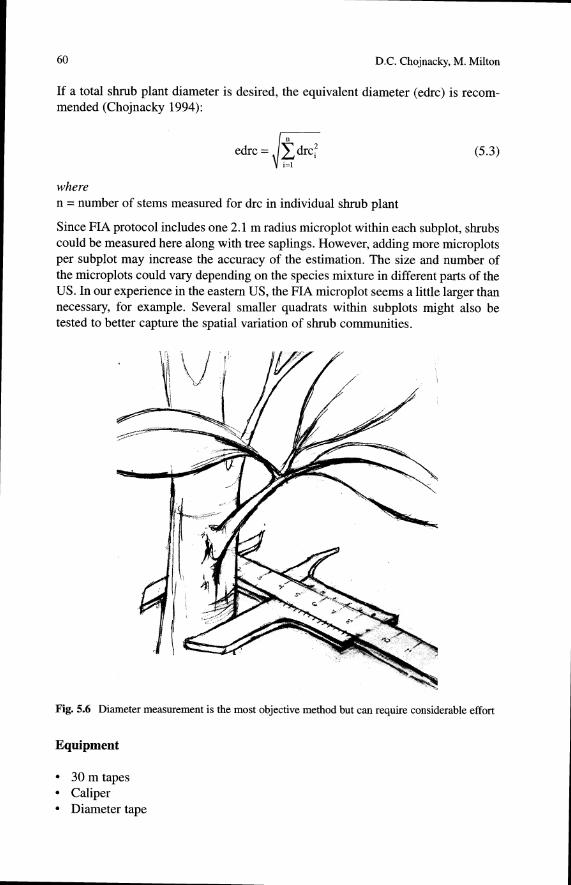
The final method also uses a fixed-area microplot but, in this case, the basal diameter of each shrub stem is measured. This is the most objective method, offering much flexibility for long-term monitoring of shrub growth and mortality. Because shrub growth is part of net primary production for understory - which can be comparable to that of trees (Nilsson and Wardle 2005) - it might be worth the extra effort to measure growth of shrub stems. However, dense mats of small-stemmed shrubs such as Vaccinium species can be particularly time-consuming to measure. Nevertheless, the shrub species definition can be modified to add a minimum diameter (5 or 10 mm, for example) below which the species would be treated as an herb and measured with a more appropriate cover-based procedure. Although there is some disagreement in the literature on where to measure shrub diameter (Ohmann et al. 1976), we advocate measuring each stem near the root collar (drc) but just above any abnormal swell (Fig. 5.6).


If a total shrub plant diameter is desired, the equivalent diameter (edrc) is recorn- mended (Chojnacky 1994):

edrc = z d r c f d ,:, where n = number of stems measured for drc in individual shrub plant

Since FIA protocol includes one 2.1 m radius microplot within each subplot, shrubs could be measured here along with tree saplings. However, adding more microplots per subplot may increase the accuracy of the estimation. The size and number of the microplots could vary depending on the species mixture in different parts of the US. In our experience in the eastern US, the FIA rnicroplot seems a little larger than necessary, for example. Several smaller quadrats within subplots might also be tested to better capture the spatial variation of shrub communities.

Fig. 5.6 Diameter measurement is the most objective method but can require considerable effort

Equipment

30 m tapes Caliper Diameter tape


Pole (generally 2 m) marked in centimeter intervals Compass Stakes or chaining pins Flagging

Procedure

On microplots, measure the drc of each shrub stem larger than some minimum diameter (probably 5 or 10 mm). For permanent plot installations, the center point of the microplot can be marked and the distance and azimuth to some or all shrub stems can be recorded for future relocation and remeasurement. In addition to species, stem status (live or dead) can be recorded to assess mortality and dead material. Height of some or all stems can also be recorded for potential regression variables for biomass estimation.

M i a m mattes 4Pte reason far choosing a m i n i m u diameter is that some skrubs---such 8s Vscci~a'%lm+an grow in low dense clumps with mmy stems smaller thm 10 mm in diameter. It is probably more reasonable ea incXude shrub stems less than 5, 8, or 30 mm in diamekr with herbaceous cover measurements rather than with ~hntbs. FurtPlermore, the compaatively little cabon accounted far by smafl shrubs does not wcAiEan-ine the exponentia1 increase in field work r e q u i ~ d to measure a11 small shmbs.

Calculations

For these data, shrub frequency, basal area, and biomass per hectare can be calculated for live and dead material in size classes. Biomass, of course, requires an appropriate drc-based equation, or one needs to constructed as described below. For illustration, we show calculation of total basal area:

where Y, = total basal area for species k (m2/ha) drc, = diameter near root collar for stem i of species k (cm) Amp = area of microplot (ha) S, = total number of stems for species k measured on microplot


Similarly, biomass could be computed with an appropriate diameter-based regression equation. Ideally, regression equations are desired for each species or for a group of similar species for different sections or areas of the U.S. However, recent theoretical work on allometric scaling (as will be discussed later) may simplify numbers of equations needed.

Summary

Diameter measurements are the most time-intensive methods presented, yet they are also the most objective, accurate, and flexible measurements that can be made for calculating shrub biomass. Such measurements can easily be combined with the FIA measurement of seedlings and saplings. The limitation of the diameter measurement method is the cost of these time-consuming measurements, particularly for dense shrub cover. However, this drawback might be balanced with carefully crafted plot sizes to minimize unnecessary measurement effort.

5.4 Summary of Recommended Methods

Table 5.1 provides a summary of the methods presented in this chapter, including strengths and limitations. For details on recommended sample sizes and dimensions for each method, consult the appropriate references.

5.5 Regression Subsampling for Carbon Estimation

The three methods described above will not estimate carbon directly without an appropriate regression equation. The best way to develop a suitable regression equation is to subsample some of the plots (or nearby plots if they are permanent) to measure actual shrub weights and then use the subsamples to develop regression equations from actual cover or diameter measurements.

Developing appropriate biomass equations is particularly important for the cover measurements (both transect and visual cover methods), because cover-to- biomass relationships can vary widely depending on the height and branching pattern of the shrub species. Therefore, considerable original research likely will be needed to develop widely applicable equations. For example, the point-intercept method might be scaled to a broad range of species by using cover (or point- intercept) measurements at various heights as variables in the equations. Likewise, visual cover estimation methods might benefit from collecting cover height variables to develop more general multiple species equations. Because only a few cover-to-weight equations exist (Olson and Martin 1981, Humphrey 1985,

Table 5.1 Comoarison of shrub biomass measurement and estimation methods

Method la-Point-intercept I b-Line-intercept 2a-Microplot variant

Method

Sample frame

Variable measured

Description

Sample size variables

Vertical vegetation canopy points (hits) intercepting perpendicular pole are tallied along transect

1-Transect intercept cover sampling

Horizontal vegetation canopy length intercepting transect is measured

Transect

Cover

3- Diameter measurement sampling Fixed-area microplot

Diameter

Transect

Cover

2-Visual cover sampling

Overhead vegetation cover is visually estimated on microplot

Fixed-area microplot

Cover

Transect length and numbers; sample points per transect

Overhead vegetation cover is visually estimated on small quadrats systematically spaced along one or more transects

Fixed-area quadrat

Cover

Transect length and numbers

Shrub stem diameters larger than some threshold are measured at drc on microplot

Microplot area and number per subplot

Microplot area and number per subplot

Quadrat area and number per transect; transects per sub~lot

Biomass calculations

Strengths

needed transects; then biomass-to- cover equation needed

Objective; rapid; easy to Objective; rapid; easy to teach;

new biomass equations

Most rapid; easy; widely used

Cover estimated directly but biomass-to-cover equation needed.

Rapid; opportunity to statistically assess many small samples

Cover estimated directly but biomass-to-cover equation needed

Biomass-to-diameter equation needed

Objective; most accurate and suitable for use in biomass equations; flexible for other long- term monitoring needs

(continued)


Mitchell et al. 1987, Gilliam and Turrill 1993, Means et al. 1994), considerable effort on subsampling should be planned until a pool of equations becomes available.

Developing these relationships for the transect methods will take extra thought, because transect point- and line-intercept methods cannot estimate biomass directly. Instead, two sampling frames likely are needed where biomass is estimated from fixed-areas, which will need to be related to cover measured on transects for the same areas. For example, cover that is measured on parallel transects or other patterns of transects can be matched to biomass that is estimated for the same area. Measurement of shrub biomass for large areas will likely be too costly; hence, microplots or quadrats would be needed to subsample biomass for the entire area sampled by transects. Rectangular belts around each transect could also be considered for estimating biomass. For certain conditions, there is a transect method pioneered by Meeuwig and Budy (1981) for estimating biomass of shrubby pinyon-juniper trees; this method might be useful for developing shrub biomass equations. We did not present Meeuwig and Budy's method here for shrub carbon estimation because their method requires simple plant communities where individual crown diameters can be easily identified; however, it might be useful for verifying cover-to-biomass regressions for transect methods.

Basal (diameter) area (BA) measurement is probably the most robust method for grouping many species into a few biomass equations, because diameter-to- weight is a strong empirical relationship (Yandle and Wiant 1981). Also, diameter-to-weight relationships have a theoretical basis in allometric scaling theory (Enquist and Niklas 2001,2002) (see sidebar). However, shrub biomass equations do not exist for all species; some are scattered throughout the forestry, range, and ecology literature (Tefler 1969, Brown 1976, Brown and Marsden 1976, Ohmann et al. 1976, Alaback 1986, Elliott and Clinton 1993). A comprehensive summary is included in BIOPAK software (Means et al. 1994) for Pacific Northwest species. As recommended for cover measurement, considerable effort on subsampling should be planned until more diameter-to-biomass equations become available.

ABemeMc &wry suppsw me %cientists who &eveXo@d Xrses &om n861Prdly KCUS- riag seworb. For exmple, &e Iu~g c h u l a t o ~ syskm md me or s h b braneEng f;oll~w simik &wv shows g m ~ s e far tree biomss es;tim&oa even ferr mu& m s (Chr%jnw@ 2002), wgch hpEes it m y &so be wo&wEle for sbmbs fA&pM from N m Fork E m s Q1IT2%%9).

(continued)


5.6 Biomass Measurements

Biomass measurement for constructing equations can be done by destructively cut- ting and weighing entire shrub plants or by using various subsampling techniques to cut and weigh plant portions (Bonham 1989, p. 228; Gregoire et al. 1995). If a subsampling technique is used, we recommend that the subsampling scheme be tested against entire plant harvesting to document the method's effectiveness. If a subsample of plots is routinely harvested as part of the sample design (by using classical regression sampling), we still recommend that auxiliary regression equations for the weight data be published. This will speed the daunting task of developing good weight relationships for all shrub species. As more shared data become available, perhaps allometric scaling or other theories can be applied to speed the process of studying one species at time at a few specific sites. Also, if biomass data


are collected, it would be useful to check the commonly held assumption that carbon is indeed 50% of dry biomass for all species.

5.7 Applying the Equations: An Example

An exhaustive meta-analysis of shrub biomass equations is beyond the scope of this chapter but examples are given to illustrate how our methods might be applied to estimate carbon in shrubs from cover or diameter measurements. Each particular application will require careful consideration of equations selected; however, examples from two existing studies are provided as a conceptual stepping stone for developing specific methodology that is appropriate to varying situations in different places.

Ideally, both the equations and the data developed would come from the same section or region of the US, unlike our situation in which the equations were developed for West Coast species and the data were collected on East Coast shrub species. Therefore, our specific results are less the focus for this chapter than the demonstration of the methods.

For our example, the equations in BIOPAK (Means et al. 1994) were summarized in a meta-analysis (as done for trees in Jenkins et al. 2003) into two equations for either cover or basal diameter measurement:

biomass, = Exp [-3.96457 + 1.08631 In (cover)] biomass, = Exp [-3.42620 + 2.5031 In (drc)]

where biomass, = total shrub dry weight (Mgha) biomass, = individual shrub stem or plant dry weight (kglplant) cover = percent shrub cover In = natural logarithm drc = basal diameter of each shrub stem near root collar (cm)

These equations were then applied to nine vegetation plots measured for both cover and drc in eastern hardwood forests in national parks near Washington, DC. Primary species included Kalmia latifolia, Lindera benzoin, Vaccinium species, and Viburnum species. The point-intercept method was used to measure cover up to 2 m in height on three 18 m transects sampled at 1 m intervals. Basal stem diameters (drc) were measured on three 4 m radius microplots within the same area for all shrub stems 5 mm and larger. The sample area for both methods was an 18 m cir- cular plot where the transects radiated out from the center at 120" angles. Individual biomass measurements were summed and appropriately expressed (using sample weights) to arrive at biomass per hectare.

Results of the test are informative and illustrate some of what to bear in mind when estimating shrub carbon (Table 5.2). First, the large differences in biomass between the coverftransect and diameterlplot sampling methods are likely due to the inaccu- racy of West Coast auxiliary equations for East Coast shrub species. The cover


Table 5.2 Comparison of two methods for estimating shrub biomass from auxiliary equations applied to diameter and cover measurements made on plots in national parks near Washrrton. DC

Drc plot Point-intercept measurement- measurement Converted

Plot information summary summary biomass*

Point- Diameter intercept- measurement

Stems Qmd Cover Height cover (drc)

No. Shrub T y ~ e Park No./ha cm % m - - - - ~ n / h ~ - - - -

Kallat Prince 1,658 William, VA

Kallat Rock Creek, 6,565 DC

Linbed Rock Creek, 20,961 VacNib DC

Linbed Catoctin, 39,689 VacNib MD

Kallat Catoctin, 53 1 MD

LinbenNacl Rock Creek, 3,7 14 Vib DC

LinbenNacl Rock Creek, 1,857 Vib DC

LinbenNacl Catoctin, 3,7 14 Vib MD

Linbenl Rock Creek, 66 VacNib DC

Species codes: Kallat-(Kalmia latifolia), Linben-(Lindera benzoin), Vac-(Vaccinium species), V i b (Wbumum species); Abbreviations: qmd=quadratic mean stem diameter, drc=diameter at root collar, cover=upper layer cover, height=height of highest layer; * Individual measurements were summed and converted to total forest dry weight using equation 5.5 and appropriate area expansion.

equation is from a conservative meta-analysis that combines low ground shrubs with some taller shrubs; it limits predictions to less than 3 Mglha no matter how much cover is actually present. Had height of cover layer or additional cover layers been included, the equation would have been more flexible. On the other hand, the diameter-based (drc) equation is probably more robust (and realistic), producing a larger and wider range of results. Therefore, these results illustrate that appropriate and realistic biomass equations are key to good carbon estimates, regardless of which method is used. Although developing good cover-to-biomass regressions will be quite difficult, costly, and time-consuming, the positive trade-off is that good equations will enable the use of rapid cover measurements from that point on.

Although not discernible in Table 5.2, the test also revealed that the largest shrub, mountain laurel (Kallat), accounted for considerable difference between the two methods. For the sake of illustration, if mountain laurel is left out of the


Table 5.3 Comparison of two methods for estimating shrub biomass from auxiliary equations, with mountain laurel (Kalmia latifolia) dropped from the analysis

Plot information Converted biomass*

Point-intercept cover Diameter measurement (drc)

Number Park ------. Mg/ha ------

PO 1 Prince William, VA 0.1 0.5 SO1 Rock Creek, DC 0.5 0.6 NO4 Rock Creek, DC 2.0 10.7 TO2 Catoctin, MD 1.6 0.9 TO 1 Catoctin, MD 0.0 0.0 CO1 Rock Creek, DC 0.5 0.6 C06 Rock Creek, DC 0.1 0.5 TO3 Catoctin, MD 0.0 0.3 C03 Rock Creek. DC 0.0 0.0

* Individual measurements were summed and converted to total forest dry weight using equation 5.5 and appropriate area expansion.

previous analysis, the diameter measurement and cover methods are more comparable (Table 5.3) because there is less mixing of high and low s h b s . However, even here the largest difference in estimated biomass (plot N04) can again be attrib- uted to many small stems of spice bush (Lindera) that add up to more biomass than would be obtained from transect cover conversion.

While there is no way of stating here for certain which method will be best for a particular project, the diameter measurement method generally will be the most sensitive because actual diameters tend to be directly proportional to biomass; thus our preference for diameter measurement (drc) as the most robust method. However, the cover methods also can be used to provide reasonable estimates if some work is done to develop separate equations for individual species groups; inclusion of height and/or more cover layers also might make the equations more robust.

5.8 Summary

A reasonable estimate of carbon in shrubs can be achieved by combining general cover or diameter measurements (using transects or microplots arranged within FIA subplots) with regression subsampling. Stem diameter measurements using microplots seem to provide the most robust data for estimating biomass (and by extension, carbon). However, these measurements require the most field time; diameter-to-biomass equations are lacking for many species, which will require considerable research work for wide application of this method; and more pilot study should be done to determine optimum size and number of rnicroplots.

More rapid measurements of cover also can be used when appropriate, realistic cover-to-biomass equations are developed. The point-intercept method - which


inherently gives cover layer and height data - might be most advantageous for developing robust cover-to-biomass relationships. This method offers a rapid but objective procedure for estimating shrub cover for individual species by layers. Although corresponding biomass equations must be developed, there seems to be considerable opportunity to develop such equations from a range of variables including cover by species at a variety of layer heights.

The need to accurately estimate carbon in shrubs will become even more vital in the future as land use and global climate changes increasingly alter both forested and non-forested ecosystems. Such changes will have implications for wildlife, biodiversity, nutrient cycling, fire, and other management issues where carbon sequestration, especially in soils, may become key objectives. We have summarized three methods that might be used to estimate carbon in shrubs. The job now is to develop appropriate equations and workable field measurement techniques that together will enable researchers and managers to measure carbon in shrubs quickly, consistently, and rigorously in the future.

Acknowledgements We gratefully acknowledge the assistance of the National Capital Region of the U. S. Department of the Interior, National Park Service, for sharing data used in example calculations; the Northern Global Change Program of the U.S. Department of Agriculture, Forest Service, for financial support; Mary Carr of the Forest Service, CAT Publishing Arts, for editing the manuscript; Michal J. Chojnacky of George Washington University for the illustrations; and Kristen Thrall of the Forest Service, Recreation Solutions, for graphics assistance.

Literature Cited

Alaback PB (1986) Biomass regression equations for understory plants in coastal Alaska: effects of species and sampling design on estimates. Northwest Science 60(2): 90-102

Bonham CD (1989) Measurements for terrestrial vegetation. New York: Wiley, 354 p Bechtold WA, Patterson PA (Eds.) (2005) The enhanced Forest Inventory and Analysis p r o g r a m

national sampling design and estimation procedures. Gen. Tech. Rep. SRS-80. Asheville, NC: U.S. Department of Agriculture, Forest Service, Southern Research Station, 85 p

Brown JK (1976) Estimating shrub biomass from basal stem diameters. Canadian Journal of Forest Research 6: 153-158

Brown JK, Marsden MA (1976) Estimating fuel weights of grasses, forbs, and small woody plants. Res. Note. INT-210. Ogden, UT: U.S. Department of Agriculture, Forest Service, Intermountain Forest and Range Experiment Station, 11 p. www.fs.fed.usldmain~pubs/invent~ries/inrlint~m~pdf

Canfield R (1941) Application of the line-interception method in sampling range vegetation. Journal of Forestry 39: 388-394

Chojnacky DC (1994) Volume equations for New Mexico's pinyon-juniper dryland forests. Research Paper INT-471. Ogden, UT: U.S. Department of Agriculture, Forest Service, Intermountain Research Experiment Station, 10 p

Chojnacky DC (1998) Double sampling for stratification: a forest inventory application in the Interior West. Res. Pap. RMRS-RP-7. Ogden, UT: U.S. Department of Agriculture, Forest Service, Rocky Mountain Research Station, 15 p

Chojnacky DC (2002) Allometric scaling theory applied to FIA biomass estimation. In: McRoberts RE, Reams GA, Van Deusen PC, Moser JW (Eds.) Proceedings of third annual forest inventory and analysis symposium, 17-19 October 2001, Traverse City, MI. Gen. Tech. Rep. NC-230. St. Paul, MN: U.S. Department of Agriculture, Forest Service, North Central Research Station, pp. 96102


Cochran WG (1977) Sampling Techniques. Third edn. New York: Wiley, 428 p Daubenmire RF (1959) Canopy coverage method of vegetation analysis. Northwest Science 33: 4 3 4 4 Diersing VE, Shaw RB, Tazik DJ (1992) U.S. A m y land condition-trend analysis (LCTA) pro-

gram. Environmental Management 16: 405414 Elliott KJ, Clinton BD (1993) Equations for estimating biomass of herbaceous and woody vegeta-

tion in early-successional southern Appalachian pine-hardwood forests. Res. Note SE-365. Asheville, NC: U.S. Department of Agriculture, Forest Service, Southeastern Forest Experiment Station, 7 p

Elzinga, CL, Salzer DW, Willoughby JW (1998) Measuring and monitoring plant populations. BLM Technical Reference 1730-1. Denver, CO: Bureau of Land Management, 477 p

Enquist BJ, Niklas KJ (2001) Invariant scaling relations across tree-dominated communities. Nature 410: 655-660

Enquist BJ, Niklas KJ (2002) Global allocation rules for biomass partitioning in seed plants. Science 295: 1517-1520

Forest Inventory and Analysis m] (2002) Phase 3 field manual-vegetation diversity and structure, March 2002. U.S. Department of Agriculture, Forest Service, Forest Inventory and Analysis program, 20 p. http://fia.fs.fed.us/Itbrary/field-guides-methods-proc/docs/p3sec13~02-03~pub.pdf

Forest Inventory and Analysis (FIA) (2004a) FIA tree species codes. In: National core field guide, volume 1: field data collection procedures for phase 2 plots, appendix 3, January 2004. U.S. Department of Agriculture, Forest Service, Forest Inventory and Analysis Program, pp. 151-163 http://fia.fs.fed.us/library/field-guides-methods-proc/docs/core~ver~2-0~0l~04.pdf [accessed June 21, 20051

Forest Inventory and Analysis (FIA) (2004b) Phase 3 field manual--down woody materials, March 2004. U.S. Department of Agriculture, Forest Service, Forest Inventory and Analysis program, 38 p. http://www.fia.fs.fed.us/library/field-guides-methods-proc/docs/p3~2-0~secl4~ 3-04.pdf [accessed December 1, 20051

Forest Inventory and Analysis (FIA) (2005) Homepage of U.S. Department of Agriculture, Forest Service, Forest Inventory and Analysis Program. [accessed June 14,20051

Gilliam FS, Tumll NL (1993) Herbaceous layer cover and biomass in a young versus a mature stand of a central Appalachian hardwood forest. Bulletin Torrey Botanical Club 120: 445450

Gregoire TG, Valentine HT, Furnival GM (1995) Sampling methods to estimate foliage and other characteristics of individual trees. Ecology 76(4): 118 1-1 194

Hanley TA (1978) A comparison of the line-interception and quadrat estimation methods for determining shrub canopy coverage. Journal of Range Management 31(1): 60-62

Heady HF, Gibbens RP, Powell RW (1959) A comparison of the charting, line intercept, and line point methods of sampling shrub types of vegetation. Journal of Range Management 12(4): 180-188

Humphrey DL (1985) Use of biomass predicted by regression from cover estimates to compare vegetational similarity of sagebrush-grass sites. Great Basin Naturalist 45(1): 94-98

Jenkins JC, Chojnacky DC, Heath LS, Birdsey RA (2003) National-scale biomass estimation for United States tree species. Forest Science 49(1): 12-35

Kimble JM, Heath LS, Birdsey RA (2002) The potential of U.S. forest soils to sequester carbon and mitigate the greenhouse effect. Washington, DC: CRC Press, 429 p

Korb, JE, Covington WW, Fule PZ (2003) Sampling techniques influence understory plant trajec- tories after restoration: an example from ponderosa pine restoration. Restoration Ecology 1 l(4): 504-515

Kort J, Turnock B (2003) Biomass production and carbon fixation by prairie shelterbelts: a green plan project. Agriculture and Agri-Food Canada, Supplementary Report 96-5 http://www.agr. gc.ca/pfra/shelterbelt/shbpub63.htm [accessed June 21, 20051

Lohr SL (1999) Sampling: design and analysis. Pacific Grove, CA: Duxbury Press, 494 p McMillin JD, Allen KK (2003) Effects of Douglas-fir beetle (Coleoptera: Scolytidae) infestations

on forest overstory and understory conditions in western Wyoming. Western North American Naturalist 63(4): 498-506


Means J, Hansen H, Koerper G, Alaback P, Klopsch M (1994) Software for computing plant biomass- BIOPAK users guide. Gen. Tech. Rep. PNW-GTR-340. Portland, OR: U.S. Department of Agriculture, Forest Service, Pacific Northwest Research Station

Meeuwig RO, Budy JD (1981) Point- and line-intersect sampling in pinyon and Utah juniper. Paper INT-104. Ogden, UT: U.S. Department of Agriculture, Forest Service, Intermountain Forest and Range Experiment Station, 38 p

Mitchell, JE, Bartling PNS, O'Brien RO (1987) Understory cover-biomass relationships in the Front Range ponderosa pine zone. Research Note RM-471. Fort Collins, CO: U.S. Department of Agriculture, Forest Service, Rocky Mountain Forest and Range Experiment Station. 5 p www.fs.fed.us/dmain/pubs/inventories/rm-m.pdf.

Nilsson MC, Wardle DA (2005) Understory vegetation as a forest ecosystem driver: evidence from the northern Swedish boreal forest. Frontiers in Ecology and the Environment. 8(30): 421428-

Ohmann LF, Grigal DF, Brander RB (1976) Biomass estimation for five shrubs from northeastern Minnesota. Journal Series 9468. St. Paul, MN: University of Minnesota. Minnesota Agriculture Experimentation Station, 11 p

Olson CM, Martin RE (1981) Estimating biomass of shrubs and forbs in central Washington Douglas-fir stands. Res. Note PNW-380. Portland, OR: U.S. Department of Agriculture, Forest Service, Pacific Northwest Research Station, 6 p

Peet RK, Wentworth TR, White PS (1998) A flexible multipurpose method for recording vegetation composition and structure. Castanea 63: 262-274

Sweeney BA, Cook JE (2001) A landscape-level assessment of understory diversity in upland forest of the North-Central Wisconsin, USA. Landscape Ecology 16: 55-69

Small CJ, McCarthy BC (2002) Spatial and temporal variability of herbaceous vegetation in an eastern deciduous forest. Plant Ecology 164: 37-48

Tefler ES (1969) Weight-diameter relationships for 22 woody plant species. Canadian Journal of Botany 47: 1851-1855

Yandle DO, Wiant HV (1981) Estimation of plant biomass based on the allometric equation. Canadian Journal Forestry Research 11: 833-834

chapter 5 measuring carbon in shrubs - nitc - north · pdf file ·...

Documents