chapter 5 failures resulting from static loading lecture slides the mcgraw-hill companies © 2012
TRANSCRIPT

Chapter 5
Failures Resulting from Static Loading
Lecture Slides
The McGraw-Hill Companies © 2012
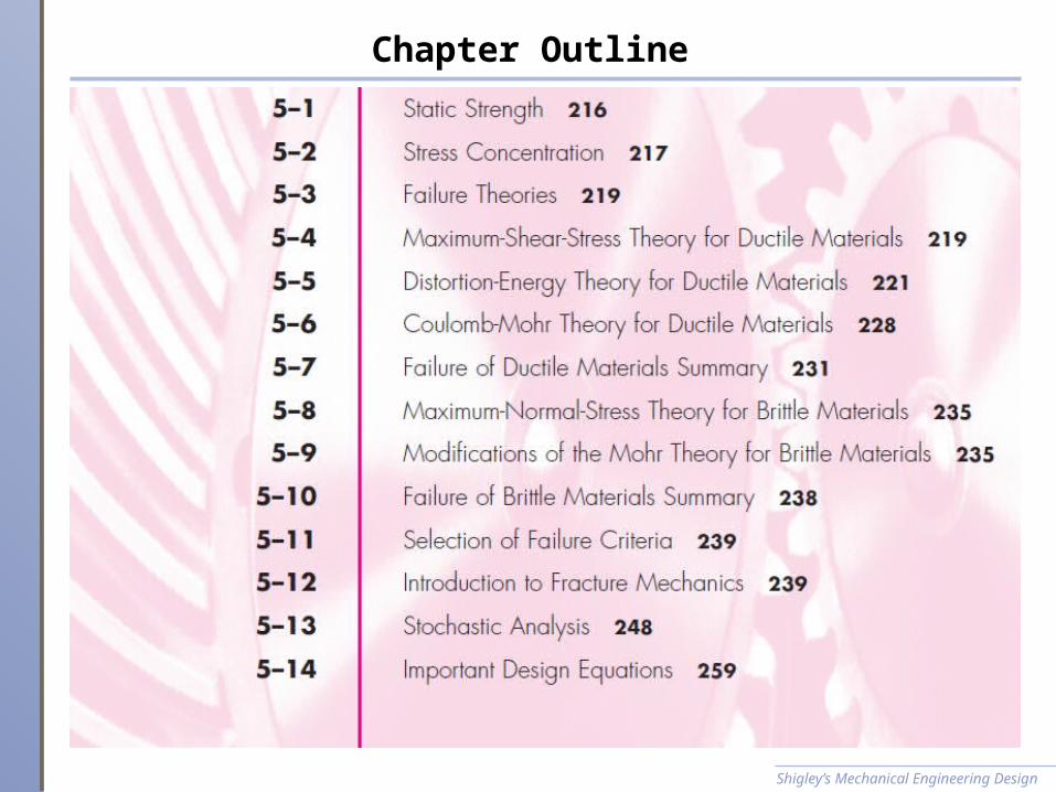
Chapter Outline
Shigley’s Mechanical Engineering Design

Failure Examples
Failure of truck driveshaft spline due to corrosion fatigue
Shigley’s Mechanical Engineering Design
Fig. 5–1

Failure Examples
Impact failure of a lawn-mower blade driver hub.The blade impacted a surveying pipe marker.
Shigley’s Mechanical Engineering Design
Fig. 5–2

Failure Examples
Failure of an overhead-pulley retaining bolt on a weightlifting machine.
A manufacturing error caused a gap that forced the bolt to take the entire moment load.
Shigley’s Mechanical Engineering Design
Fig. 5–3

Failure Examples
Chain test fixture that failed in one cycle. To alleviate complaints of excessive wear, the manufacturer decided to
case-harden the material (a) Two halves showing brittle fracture initiated by stress concentration (b) Enlarged view showing cracks induced by stress concentration at
the support-pin holesShigley’s Mechanical Engineering Design
Fig. 5–4

Failure Examples
Valve-spring failure caused by spring surge in an oversped engine.
The fractures exhibit the classic 45 degree shear failure
Shigley’s Mechanical Engineering Design
Fig. 5–5
Static Strength
Usually necessary to design using published strength valuesExperimental test data is better, but generally only warranted
for large quantities or when failure is very costly (in time, expense, or life)
Methods are needed to safely and efficiently use published strength values for a variety of situations
Shigley’s Mechanical Engineering Design

Stress Concentration
Localized increase of stress near discontinuitiesKt is Theoretical (Geometric) Stress Concentration Factor
Shigley’s Mechanical Engineering Design

Theoretical Stress Concentration Factor
Graphs available for standard configurations
See Appendix A–15 and A–16 for common examples
Many more in Peterson’s Stress-Concentration Factors
Note the trend for higher Kt at sharper discontinuity radius, and at greater disruption
Shigley’s Mechanical Engineering Design

Stress Concentration for Static and Ductile Conditions
With static loads and ductile materials◦Highest stressed fibers yield (cold work)◦ Load is shared with next fibers◦Cold working is localized◦Overall part does not see damage unless ultimate strength is
exceeded◦ Stress concentration effect is commonly ignored for static
loads on ductile materialsStress concentration must be included for dynamic loading (See
Ch. 6)Stress concentration must be included for brittle materials,
since localized yielding may reach brittle failure rather than cold-working and sharing the load.
Shigley’s Mechanical Engineering Design

Need for Static Failure Theories
Uniaxial stress element (e.g. tension test)
Multi-axial stress element ◦One strength, multiple stresses◦How to compare stress state to single strength?
Shigley’s Mechanical Engineering Design
Strength Sn
Stress

Need for Static Failure Theories
Failure theories propose appropriate means of comparing multi-axial stress states to single strength
Usually based on some hypothesis of what aspect of the stress state is critical
Some failure theories have gained recognition of usefulness for various situations
Shigley’s Mechanical Engineering Design

Maximum Normal (Principal) Stress Theory
Theory: Yielding begins when the maximum principal stress in a stress element exceeds the yield strength.
For any stress element, use Mohr’s circle to find the principal stresses.
Compare the largest principal stress to the yield strength.Often the first theory to be proposed by engineering students. Is it a good theory?
Shigley’s Mechanical Engineering Design

Maximum Normal (Principal) Stress Theory
Experimental data shows the theory is unsafe in the 4th quadrant.
This theory is not safe to use for ductile materials.
Shigley’s Mechanical Engineering Design

Maximum Shear Stress Theory (MSS)
Theory: Yielding begins when the maximum shear stress in a stress element exceeds the maximum shear stress in a tension test specimen of the same material when that specimen begins to yield.
For a tension test specimen, the maximum shear stress is 1 /2.
At yielding, when 1 = Sy, the maximum shear stress is Sy /2 .
Could restate the theory as follows:◦ Theory: Yielding begins when the maximum shear stress in a
stress element exceeds Sy/2.
Shigley’s Mechanical Engineering Design

Maximum Shear Stress Theory (MSS)
For any stress element, use Mohr’s circle to find the maximum shear stress. Compare the maximum shear stress to Sy/2.
Ordering the principal stresses such that 1 ≥2 ≥3,
Incorporating a design factor n
Or solving for factor of safety
Shigley’s Mechanical Engineering Design
max
/ 2ySn

Maximum Shear Stress Theory (MSS)
To compare to experimental data, express max in terms of principal stresses and plot.
To simplify, consider a plane stress stateLet A and B represent the two non-zero principal stresses, then
order them with the zero principal stress such that 1 ≥2 ≥3
Assuming A ≥B there are three cases to consider
◦Case 1: A ≥B ≥
◦Case 2: A ≥ ≥B
◦Case 3: 0 ≥A ≥ B
Shigley’s Mechanical Engineering Design

Maximum Shear Stress Theory (MSS)
Case 1: A ≥B ≥
◦ For this case, 1 = A and 3 = 0
◦ Eq. (5–1) reduces to A ≥ Sy
Case 2: A ≥ ≥B
◦ For this case, 1 = A and 3 = B
◦ Eq. (5–1) reduces to A − B ≥ Sy
Case 3: 0 ≥A ≥ B
◦ For this case, 1 = and 3 = B
◦ Eq. (5–1) reduces to B ≤ −Sy
Shigley’s Mechanical Engineering Design

Maximum Shear Stress Theory (MSS)
Plot three cases on principal stress axes
Case 1: A ≥B ≥
◦ A ≥ Sy
Case 2: A ≥ ≥B
◦ A − B ≥ Sy
Case 3: 0 ≥A ≥ B
◦ B ≤ −Sy
Other lines are symmetric cases
Inside envelope is predicted safe zone
Shigley’s Mechanical Engineering Design
Fig. 5–7

Maximum Shear Stress Theory (MSS)
Comparison to experimental data
Conservative in all quadrants
Commonly used for design situations
Shigley’s Mechanical Engineering Design

Distortion Energy (DE) Failure Theory
Also known as:◦Octahedral Shear Stress◦ Shear Energy◦Von Mises◦Von Mises – Hencky
Shigley’s Mechanical Engineering Design

Distortion Energy (DE) Failure Theory
Originated from observation that ductile materials stressed hydrostatically (equal principal stresses) exhibited yield strengths greatly in excess of expected values.
Theorizes that if strain energy is divided into hydrostatic volume changing energy and angular distortion energy, the yielding is primarily affected by the distortion energy.
Shigley’s Mechanical Engineering Design
Fig. 5–8

Distortion Energy (DE) Failure Theory
Theory: Yielding occurs when the distortion strain energy per unit volume reaches the distortion strain energy per unit volume for yield in simple tension or compression of the same material.
Shigley’s Mechanical Engineering Design
Fig. 5–8

Deriving the Distortion Energy
Hydrostatic stress is average of principal stresses
Strain energy per unit volume,Substituting Eq. (3–19) for principal strains into strain energy
equation,
Shigley’s Mechanical Engineering Design

Deriving the Distortion Energy
Strain energy for producing only volume change is obtained by substituting av for 1, 2, and 3
Substituting av from Eq. (a),
Obtain distortion energy by subtracting volume changing energy, Eq. (5–7), from total strain energy, Eq. (b)
Shigley’s Mechanical Engineering Design
Deriving the Distortion Energy
Tension test specimen at yield has 1 = Sy and 2 = 3 =0
Applying to Eq. (5–8), distortion energy for tension test specimen is
DE theory predicts failure when distortion energy, Eq. (5–8), exceeds distortion energy of tension test specimen, Eq. (5–9)
Shigley’s Mechanical Engineering Design

Von Mises Stress
Left hand side is defined as von Mises stress
For plane stress, simplifies to
In terms of xyz components, in three dimensions
In terms of xyz components, for plane stress
Shigley’s Mechanical Engineering Design

Distortion Energy Theory With Von Mises Stress
Von Mises Stress can be thought of as a single, equivalent, or effective stress for the entire general state of stress in a stress element.
Distortion Energy failure theory simply compares von Mises stress to yield strength.
Introducing a design factor,
Expressing as factor of safety,
Shigley’s Mechanical Engineering Design
ySn

Octahedral Stresses
Same results obtained by evaluating octahedral stresses.Octahedral stresses are identical on 8 surfaces symmetric to the
principal stress directions.Octahedral stresses allow representation of any stress situation
with a set of normal and shear stresses.
Shigley’s Mechanical Engineering Design
Principal stress element with single octahedral plane showing
All 8 octahedral planes showing

Octahedral Shear Stress
Octahedral normal stresses are normal to the octahedral surfaces, and are equal to the average of the principal stresses.
Octahedral shear stresses lie on the octahedral surfaces.
Shigley’s Mechanical Engineering Design
Fig. 5–10

Octahedral Shear Stress Failure Theory
Theory: Yielding begins when the octahedral shear stress in a stress element exceeds the octahedral shear stress in a tension test specimen at yielding.
The octahedral shear stress is
For a tension test specimen at yielding, 1 = Sy , 2 = 3 = 0. Substituting into Eq. (5–16),
The theory predicts failure when Eq. (5–16) exceeds Eq. (5–17). This condition reduces to
Shigley’s Mechanical Engineering Design

Failure Theory in Terms of von Mises Stress
Equation is identical to Eq. (5–10) from Distortion Energy approach
Identical conclusion for:◦Distortion Energy ◦Octahedral Shear Stress◦ Shear Energy◦Von Mises◦Von Mises – Hencky
Shigley’s Mechanical Engineering Design
ySn

DE Theory Compared to Experimental Data
Plot von Mises stress on principal stress axes to compare to experimental data (and to other failure theories)
DE curve is typical of dataNote that typical equates
to a 50% reliability from a design perspective
Commonly used for analysis situations
MSS theory useful for design situations where higher reliability is desired
Shigley’s Mechanical Engineering Design
Fig. 5–15

Shear Strength Predictions
Shigley’s Mechanical Engineering Design
For pure shear loading, Mohr’s circle shows that A = −B = Plotting this equation on principal stress axes gives load line for
pure shear case Intersection of pure shear load line with failure curve indicates
shear strength has been reachedEach failure theory predicts shear strength to be some fraction of
normal strength
Fig. 5–9

Shear Strength Predictions
Shigley’s Mechanical Engineering Design
For MSS theory, intersecting pure shear load line with failure line [Eq. (5–5)] results in
Fig. 5–9

Shear Strength Predictions
Shigley’s Mechanical Engineering Design
For DE theory, intersection pure shear load line with failure curve [Eq. (5–11)] gives
Therefore, DE theory predicts shear strength as
Fig. 5–9

Example 5-1
Shigley’s Mechanical Engineering Design

Example 5-1
Shigley’s Mechanical Engineering Design

Example 5-1
Shigley’s Mechanical Engineering Design

Example 5-1
Shigley’s Mechanical Engineering Design

Example 5-1
Shigley’s Mechanical Engineering Design

Example 5-1
Shigley’s Mechanical Engineering Design

Example 5-1
Shigley’s Mechanical Engineering DesignFig. 5−11

Example 5-1
Shigley’s Mechanical Engineering DesignFig. 5−11

Mohr Theory
Some materials have compressive strengths different from tensile strengths
Mohr theory is based on three simple tests: tension, compression, and shear
Plotting Mohr’s circle for each, bounding curve defines failure envelope
Shigley’s Mechanical Engineering Design
Fig. 5−12

Coulomb-Mohr Theory
Curved failure curve is difficult to determine analyticallyCoulomb-Mohr theory simplifies to linear failure envelope
using only tension and compression tests (dashed circles)
Shigley’s Mechanical Engineering Design
Fig. 5−13

Coulomb-Mohr Theory
From the geometry, derive the failure criteria
Shigley’s Mechanical Engineering Design
Fig. 5−13
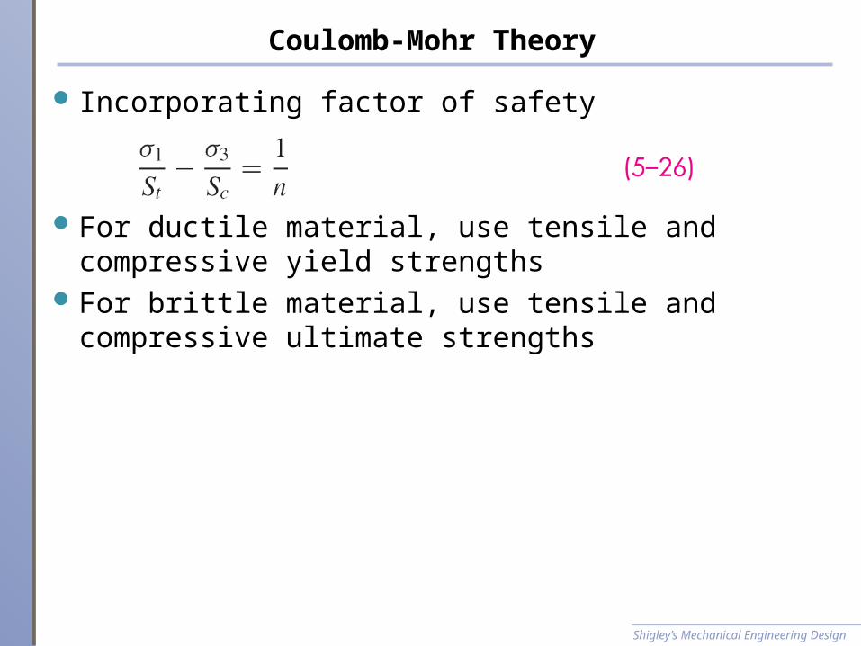
Coulomb-Mohr Theory
Incorporating factor of safety
For ductile material, use tensile and compressive yield strengthsFor brittle material, use tensile and compressive ultimate
strengths
Shigley’s Mechanical Engineering Design

Coulomb-Mohr Theory
To plot on principal stress axes, consider three casesCase 1: A ≥B ≥ For this case, 1 = A and 3 = 0
◦ Eq. (5−22) reduces to
Case 2: A ≥ ≥B For this case, 1 = A and 3 = B
◦ Eq. (5-22) reduces to
Case 3: 0 ≥A ≥ B For this case, 1 = and 3 = B
◦ Eq. (5−22) reduces to
Shigley’s Mechanical Engineering Design
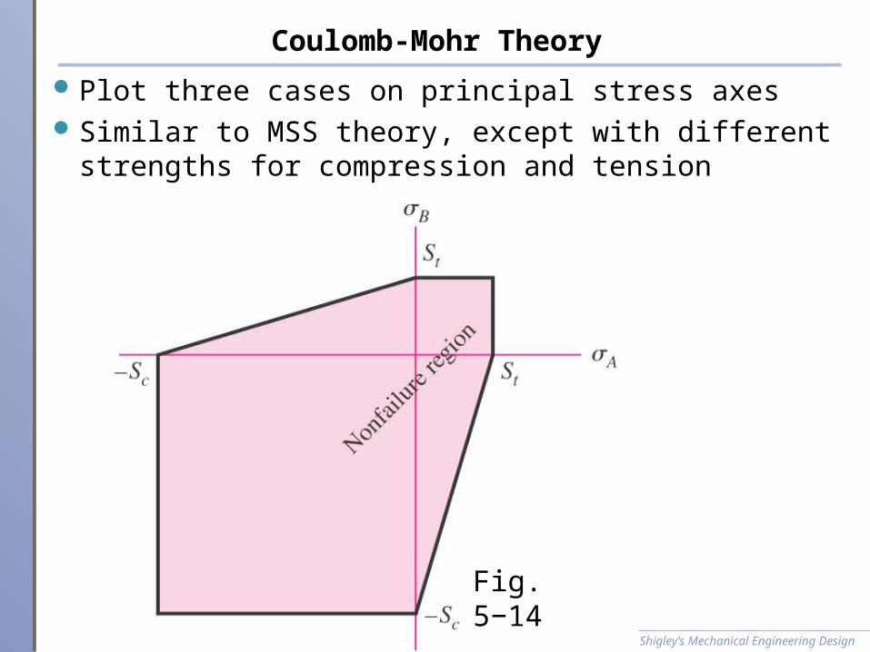
Coulomb-Mohr Theory
Plot three cases on principal stress axesSimilar to MSS theory, except with different strengths for
compression and tension
Shigley’s Mechanical Engineering Design
Fig. 5−14

Coulomb-Mohr Theory
Intersect the pure shear load line with the failure line to determine the shear strength
Since failure line is a function of tensile and compressive strengths, shear strength is also a function of these terms.
Shigley’s Mechanical Engineering Design

Example 5-2
Shigley’s Mechanical Engineering Design

Example 5-2
Shigley’s Mechanical Engineering Design

Example 5-3
Shigley’s Mechanical Engineering DesignFig. 5−16
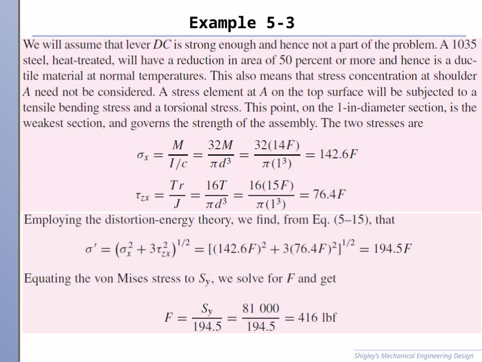
Example 5-3
Shigley’s Mechanical Engineering Design

Example 5-3
Shigley’s Mechanical Engineering Design

Example 5-4
Shigley’s Mechanical Engineering Design
Fig. 5−17

Example 5-4
Shigley’s Mechanical Engineering DesignFig. 5−17

Example 5-4
Shigley’s Mechanical Engineering Design
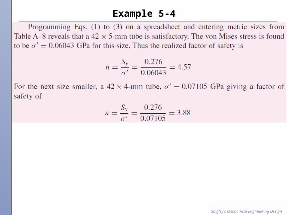
Example 5-4
Shigley’s Mechanical Engineering Design

Failure Theories for Brittle Materials
Experimental data indicates some differences in failure for brittle materials.
Failure criteria is generally ultimate fracture rather than yieldingCompressive strengths are usually larger than tensile strengths
Shigley’s Mechanical Engineering DesignFig. 5−19

Maximum Normal Stress Theory
Theory: Failure occurs when the maximum principal stress in a stress element exceeds the strength.
Predicts failure when
For plane stress,
Incorporating design factor,
Shigley’s Mechanical Engineering Design

Maximum Normal Stress Theory
Plot on principal stress axesUnsafe in part of fourth quadrantNot recommended for use Included for historical comparison
Shigley’s Mechanical Engineering DesignFig. 5−18

Brittle Coulomb-Mohr
Same as previously derived, using ultimate strengths for failureFailure equations dependent on quadrant
Shigley’s Mechanical Engineering Design
Quadrant condition Failure criteria
Fig. 5−14

Brittle Failure Experimental Data
Coulomb-Mohr is conservative in 4th quadrant
Modified Mohr criteria adjusts to better fit the data in the 4th quadrant
Shigley’s Mechanical Engineering Design
Fig. 5−19

Modified-Mohr
Shigley’s Mechanical Engineering Design
Quadrant condition Failure criteria

Example 5-5
Shigley’s Mechanical Engineering Design
Fig. 5−16

Example 5-5
Shigley’s Mechanical Engineering Design
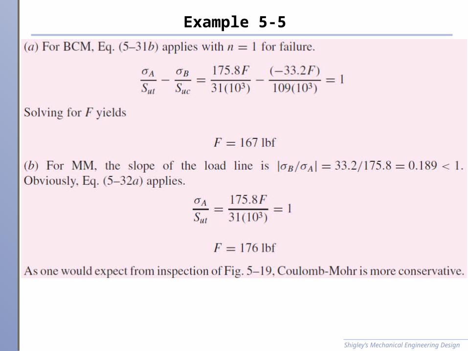
Example 5-5
Shigley’s Mechanical Engineering Design
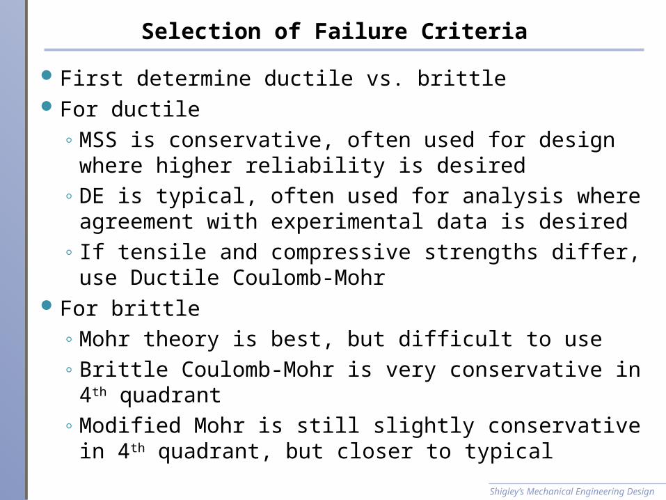
Selection of Failure Criteria
First determine ductile vs. brittleFor ductile◦MSS is conservative, often used for design where higher
reliability is desired◦DE is typical, often used for analysis where agreement with
experimental data is desired◦ If tensile and compressive strengths differ, use Ductile
Coulomb-MohrFor brittle◦Mohr theory is best, but difficult to use◦Brittle Coulomb-Mohr is very conservative in 4th quadrant◦Modified Mohr is still slightly conservative in 4th quadrant, but
closer to typical
Shigley’s Mechanical Engineering Design

Selection of Failure Criteria in Flowchart Form
Shigley’s Mechanical Engineering Design
Fig. 5−21
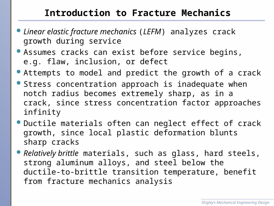
Introduction to Fracture Mechanics
Linear elastic fracture mechanics (LEFM) analyzes crack growth during service
Assumes cracks can exist before service begins, e.g. flaw, inclusion, or defect
Attempts to model and predict the growth of a crackStress concentration approach is inadequate when notch radius
becomes extremely sharp, as in a crack, since stress concentration factor approaches infinity
Ductile materials often can neglect effect of crack growth, since local plastic deformation blunts sharp cracks
Relatively brittle materials, such as glass, hard steels, strong aluminum alloys, and steel below the ductile-to-brittle transition temperature, benefit from fracture mechanics analysis
Shigley’s Mechanical Engineering Design

Quasi-Static Fracture
Though brittle fracture seems instantaneous, it actually takes time to feed the crack energy from the stress field to the crack for propagation.
A static crack may be stable and not propagate.Some level of loading can render a crack unstable, causing it to
propagate to fracture.
Shigley’s Mechanical Engineering Design

Quasi-Static Fracture
Foundation work for fracture mechanics established by Griffith in 1921
Considered infinite plate with an elliptical flawMaximum stress occurs at (±a, 0)
Shigley’s Mechanical Engineering Design
Fig. 5−22

Quasi-Static Fracture
Crack growth occurs when energy release rate from applied loading is greater than rate of energy for crack growth
Unstable crack growth occurs when rate of change of energy release rate relative to crack length exceeds rate of change of crack growth rate of energy
Shigley’s Mechanical Engineering Design

Crack Modes and the Stress Intensity Factor
Three distinct modes of crack propagation◦Mode I: Opening crack mode, due to tensile stress field◦Mode II: Sliding mode, due to in-plane shear◦Mode III: Tearing mode, due to out-of-plane shear
Combination of modes possibleOpening crack mode is most common, and is focus of this text
Shigley’s Mechanical Engineering Design
Fig. 5−23
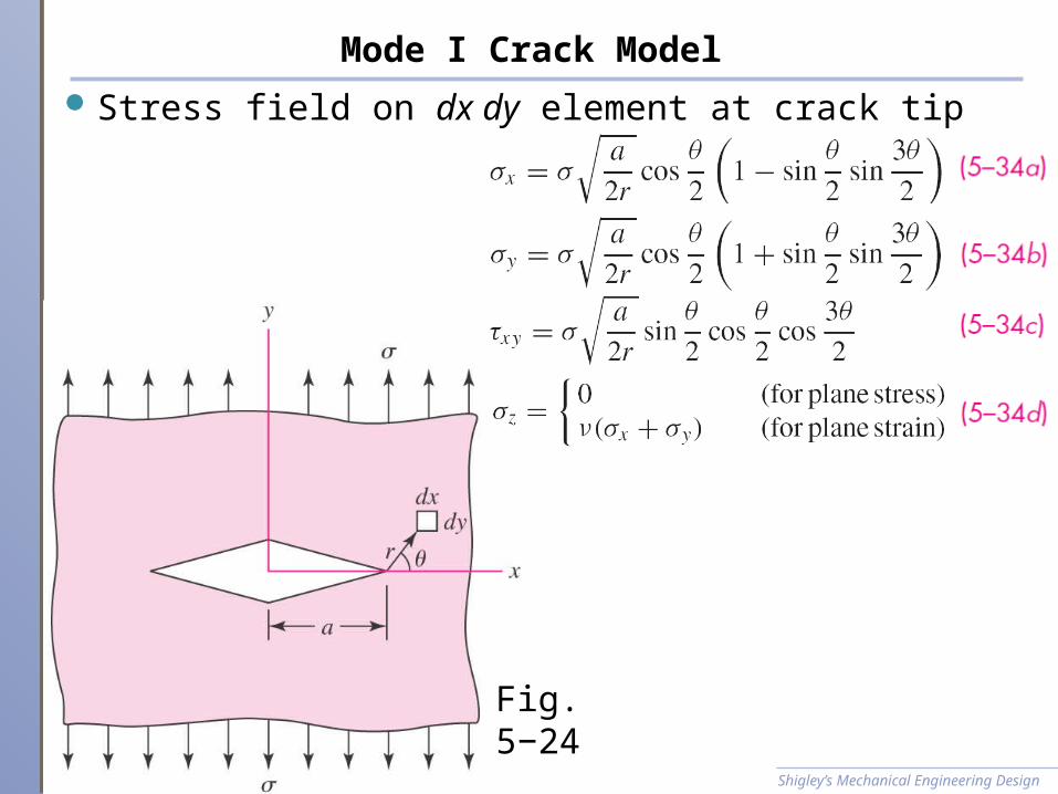
Mode I Crack Model
Stress field on dx dy element at crack tip
Shigley’s Mechanical Engineering Design
Fig. 5−24

Stress Intensity Factor
Common practice to define stress intensity factor
Incorporating KI, stress field equations are
Shigley’s Mechanical Engineering Design

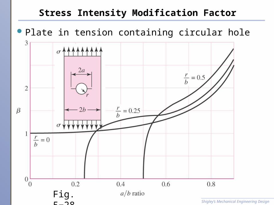
Stress Intensity Modification Factor
Stress intensity factor KI is a function of geometry, size, and shape of the crack, and type of loading
For various load and geometric configurations, a stress intensity modification factor can be incorporated
Tables for are available in the literatureFigures 5−25 to 5−30 present some common configurations
Shigley’s Mechanical Engineering Design

Stress Intensity Modification Factor
Off-center crack in plate in longitudinal tension
Solid curves are for crack tip at A
Dashed curves are for tip at B
Shigley’s Mechanical Engineering Design
Fig. 5−25

Stress Intensity Modification Factor
Plate loaded in longitudinal tension with crack at edge
For solid curve there are no constraints to bending
Dashed curve obtained with bending constraints added
Shigley’s Mechanical Engineering Design
Fig. 5−26

Stress Intensity Modification Factor
Beams of rectangular cross section having an edge crack
Shigley’s Mechanical Engineering Design
Fig. 5−27
Stress Intensity Modification Factor
Plate in tension containing circular hole with two cracks
Shigley’s Mechanical Engineering Design
Fig. 5−28

Stress Intensity Modification Factor
Cylinder loaded in axial tension having a radial crack of depth a extending completely around the circumference
Shigley’s Mechanical Engineering Design
Fig. 5−29

Stress Intensity Modification Factor
Cylinder subjected to internal pressure p, having a radial crack in the longitudinal direction of depth a
Shigley’s Mechanical Engineering Design
Fig. 5−30

Fracture Toughness
Crack propagation initiates when the stress intensity factor reaches a critical value, the critical stress intensity factor KIc
KIc is a material property dependent on material, crack mode, processing of material, temperature, loading rate, and state of stress at crack site
Also know as fracture toughness of materialFracture toughness for plane strain is normally lower than for
plain stressKIc is typically defined as mode I, plane strain fracture toughness
Shigley’s Mechanical Engineering Design

Typical Values for KIc
Shigley’s Mechanical Engineering Design

Brittle Fracture Factor of Safety
Brittle fracture should be considered as a failure mode for◦ Low-temperature operation, where ductile-to-brittle transition
temperature may be reached
◦Materials with high ratio of Sy/Su, indicating little ability to absorb energy in plastic region
A factor of safety for brittle fracture
Shigley’s Mechanical Engineering Design

Example 5-6
Shigley’s Mechanical Engineering Design

Example 5-6
Shigley’s Mechanical Engineering Design
Fig. 5−25

Example 5-6
Shigley’s Mechanical Engineering Design

Example 5-7
Shigley’s Mechanical Engineering Design

Example 5-7
Shigley’s Mechanical Engineering Design

Example 5-7
Shigley’s Mechanical Engineering DesignFig. 5−26
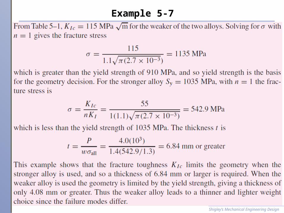
Example 5-7
Shigley’s Mechanical Engineering Design

Stochastic Analysis
Reliability is the probability that machine systems and components will perform their intended function without failure.
Deterministic relations between stress, strength, and design factor are often used due to simplicity and difficulty in acquiring statistical data.
Stress and strength are actually statistical in nature.
Shigley’s Mechanical Engineering Design

Probability Density Functions
Stress and strength are statistical in naturePlots of probability density functions shows distributionsOverlap is called interference of and S, and indicates parts
expected to fail
Shigley’s Mechanical Engineering Design
Fig. 5−31 (a)

Probability Density Functions
Mean values of stress and strength are and S
Average factor of safety is
Margin of safety for any value of stress and strength S is
The overlap area has negative margin of safety
Shigley’s Mechanical Engineering Design
Fig. 5−31 (a)

Margin of Safety
Distribution of margin of safety is dependent on distributions of stress and strength
Reliability R is area under the margin of safety curve for m > 0 Interference is the area 1−R where parts are expected to fail
Shigley’s Mechanical Engineering Design
Fig. 5−31 (b)

Normal-Normal Case
Common for stress and strength to have normal distributions
Margin of safety is m = S – , and will be normally distributedReliability is probability p that m > 0
To find chance that m > 0, form the transformation variable of m and substitute m=0 [See Eq. (20−16)]
Eq. (5−40) is known as the normal coupling equation
Shigley’s Mechanical Engineering Design

Normal-Normal Case
Reliability is given by
Get R from Table A−10The design factor is given by
where
Shigley’s Mechanical Engineering Design

Lognormal-Lognormal Case
For case where stress and strength have lognormal distributions, from Eqs. (20−18) and (20−19),
Applying Eq. (5−40),
Shigley’s Mechanical Engineering Design

Lognormal-Lognormal Case
The design factor n is the random variable that is the quotient of S/
The quotient of lognormals is lognormal. Note that
The companion normal to n, from Eqs. (20−18) and (20−19), has mean and standard deviation of
Shigley’s Mechanical Engineering Design

Lognormal-Lognormal Case
The transformation variable for the companion normal y distribution is
Failure will occur when the stress is greater than the strength, when , or when y < 0. So,
Solving for n,
Shigley’s Mechanical Engineering Design
1n

Example 5-8
Shigley’s Mechanical Engineering Design

Example 5-8
Shigley’s Mechanical Engineering Design

Example 5-8
Shigley’s Mechanical Engineering Design

Example 5-9
Shigley’s Mechanical Engineering Design

Example 5-9
Shigley’s Mechanical Engineering Design

Interference - General
A general approach to interference is needed to handle cases where the two variables do not have the same type of distribution.
Define variable x to identify points on both distributions
Shigley’s Mechanical Engineering Design
Fig. 5−32

Interference - General
Substituting 1– R2 for F2 and –dR1 for dF1,
The reliability is obtained by integrating x from – ∞ to ∞ which corresponds to integration from 1 to 0 on reliability R1.
Shigley’s Mechanical Engineering Design

Interference - General
Shigley’s Mechanical Engineering Design
where

Interference - General
Shigley’s Mechanical Engineering Design
Plots of R1 vs R2
Shaded area is equal to 1– R, and is obtained by numerical integration
Plot (a) for asymptotic distributionsPlot (b) for lower truncated distributions such as Weibull
Fig. 5−33