Chapter 5

Discrete Probability Distributions

5-2 Random Variables 1. As defined in the text, a random variable is a variable that takes on a single numerical value, determined by chance, for each outcome of a procedure. In this exercise, the random variable is the number of winning lottery tickets obtained over a 52 week period. The possible values for this random variable are 0,1,2,…,52.

2. No; the expected value does not have to be one of the values that the random variable can actually take on. The expected value is not the value most likely to occur on any given trial, but rather it is mean of the values obtained from an infinite number of trials (i.e., the weighted mean of the all the values in the population).

3. The probability distribution gives each possible non-overlapping outcome Oi of a procedure and the probability P(Oi ) associated with each of those outcomes. Since it is a certainty that one of the outcomes will occur, P(O1 or O2 or O3 or…) = 1. Since the outcomes are mutually exclusive, P(O1 or O2 or O3 or…) = P(O1) +P(O2) +P(O3) +…. Therefore, P(O1) +P(O2) +P(O3) +… = ΣP(Oi) = 1.

4. No; such a loading of a die is not possible because it would lead to probabilities larger than 1 – e.g., P(x=5 or x=6) = P(x=5) + P(x=6) = 0.5 + 0.6 = 1.1. No; the listing of these outcomes and their supposed probabilities does not constitute a probability distribution because the sum of the probabilities is 0.1 + 0.2 + 0.3 + 0.4 + 0.5 + 0.6 = 2.1, which is greater than 1.

5. a. Discrete, since such a number is limited to certain values – viz., the non-negative integers. b. Continuous, since weight can be any value on a specified continuum. c. Continuous, since height can be any value on a specified continuum. d. Discrete, since such a number is limited to certain values – viz., the non-negative integers. e. Continuous, since time can be any value on a specified continuum.

6. a. Continuous, since volume can be any value on a specified continuum. b. Discrete, since such a number is limited to certain values – viz., the non-negative integers. NOTE: One could make a case that a person could consume 1/2 of a can, or 3/4 of a can, or any portion of a can [even 1/ 2 = 0.7071… of a can] – so that the number of cans consumed is a continuous random variable. c. Discrete, since such a number is limited to certain values – viz., the non-negative integers. d. Continuous, since time can be any value on a specified continuum. e. Discrete, since such costs are limited to certain values – viz., whole numbers of cents. NOTE: If one of the conditions for a probability distribution does not hold, the formulas do not apply – and they produce numbers that have no meaning. When working with probability distributions and formulas in the exercises that follow, always keep the following important facts in mind.

108 CHAPTER 5 Discrete Probability Distributions • ΣP(x) must always equal 1.000 • Σ[x·P(x)] gives the mean of the x values and must be a number between the highest and lowest x values. • Σ[x2·P(x)] gives the mean of the x2 values and must be a number between the highest and lowest x2 values. • Σx and Σx2 have no meaning and should not be calculated • The quantity “Σ[x2·P(x)] – μ2” cannot possibly be negative – if it is, there is a mistake. • Always be careful to use the unrounded mean in the calculation of the variance, and to take the

square root of the unrounded variance to find the standard deviation.

7. The given table is a probability distribution since 0 ≤ P(x) ≤ 1 for each x and ΣP(x)=1. x P(x) x·P(x) x2 x2·P(x) μ = Σ[x·P(x)] 0 0.125 0 0 0 = 1.500, rounded to 1.5 children 1 0.375 0.375 1 0.375 σ2 = Σ[x2·P(x)] – μ2 2 0.375 0.750 4 1.500 = 3.000 – (1.500)2 3 0.125 0.375 9 1.125 = 0.750 1.000 1.500 3.000 σ = 0.866, rounded to 0.9 children

8. The given table is not a probability distribution since ΣP(x) = 0.75 ≠ 1.

9. The given table is not a probability distribution since ΣP(x) = 0.984 ≠ 1.

10. The given table is a probability distribution since 0 ≤ P(x) ≤ 1 for each x and ΣP(x)=1. x P(x) x·P(x) x2 x2·P(x) μ = Σ[x·P(x)] 0 0.528 0 0 0 = 0.599, rounded to 0.6 babies 1 0.360 0.360 1 0.360 σ2 = Σ[x2·P(x)] – μ2 2 0.098 0.196 4 0.392 = 0.885 – (0.599)2 3 0.013 0.039 9 0.117 = 0.526 4 0.001 0.004 16 0.016 σ = 0.725, rounded to 0.7 babies 5 0+ 0 25 0 1.000 0.599 0.885

11. The given table is a probability distribution since 0 ≤ P(x) ≤ 1 for each x and ΣP(x)=1. x P(x) x·P(x) x2 x2·P(x) μ = Σ[x·P(x)] 0 0.02 0 0 0 = 2.75, rounded to 2.8 TV sets 1 0.15 0.15 1 0.15 σ2 = Σ[x2·P(x)] – μ2 2 0.29 0.58 4 1.16 = 9.21 – (2.75)2 3 0.26 0.78 9 2.34 = 1.6475 4 0.16 0.64 16 2.56 σ = 1.284, rounded to 1.3 TV sets 5 0.12 0.60 25 3.00 1.00 2.75 9.21

12. The given table is a probability distribution since 0 ≤ P(x) ≤ 1 for each x and ΣP(x)=1. x P(x) x·P(x) x2 x2·P(x) μ = Σ[x·P(x)] 0 0.539 0 0 0 = 0.587, rounded to 0.6 households 1 0.351 0.351 1 0.351 σ2 = Σ[x2·P(x)] – μ2 2 0.095 0.190 4 0.380 = 0.873 – (0.587)2 3 0.014 0.042 9 0.126 = 0.528 4 0.001 0.004 16 0.016 σ = 0.727, rounded to 0.7 households 5 0+ 0 25 0 6 0+ 0 36 0 1.000 0.587 0.873

Random Variables SECTION 5-2 109 13. The given table is a probability distribution since 0 ≤ P(x) ≤ 1 for each x and ΣP(x)=1. x P(x) x·P(x) x2 x2·P(x) μ = Σ[x·P(x)] 0 0+ 0 0 0 = 6.000, rounded to 6.0 peas 1 0+ 0 1 0 σ2 = Σ[x2·P(x)] – μ2 2 0.004 0.008 4 0.016 = 37.484 – (6.000)2 3 0.023 0.069 9 0.207 = 1.484 4 0.087 0.348 16 1.382 σ = 1.218, rounded to 1.2 peas 5 0.208 1.040 25 5.200 6 0.311 1.866 36 11.196 7 0.267 1.869 49 13.083 8 0.100 0.800 64 6.400 1.000 6.000 37.484

14. The range rule of thumb suggests that “usual” values are those within two standard deviations of the mean. minimum usual value = μ – 2σ = 6.0 – 2(1.2) = 3.6 maximum usual value = μ + 2σ = 6.0+ 2(1.2) = 8.4 Yes; since 1 < 3.6, getting only one offspring pea with a green pod would be considered unusual.

15. a. P(x=7) = 0.267 b. P(x ≥ 7) = P(x=7 or x=8) = P(x=7) + P(x=8) = 0.267 + 0.100 = 0.367 c. The answer in part (b) is the one which determines whether 7 is an unusually high result. When there are several different possible outcomes, the probability of getting any one of them exactly (even the more likely ones near the middle of the distribution) may be small. An outcome is unusually high if it is in the upper tail of the distribution – i.e., if the probability of getting it or a higher value is small. d. No; since P(x ≥ 7) = 0.367 > 0.05, 7 is not an unusually high number of peas with green pods.

16. a. P(x=3) = 0.023. b. P(x ≤ 3) = P(x=3 or X=2 or x=1 or x=0) = P(x=3) = P)x=2) + P(x=1) + P(x=0) = 0.023 + 0.004 + 0+ + 0+ = 0.027 c. The answer in part (b) is the one which determines whether 3 is an unusually low result. When there are several different possible outcomes, the probability of getting any one of them exactly (even the more likely ones near the middle of the distribution) may be small. An outcome is unusually low if it is in the lower tail of the distribution – i.e., if the probability of getting it or a lower value is small. d. Yes; since P(x ≤ 3) = 0.027 ≤ 0.05, 3 is an unusually low number of peas with green pods.

17. a. The given table is a probability distribution since 0≤ P(x) ≤ 1 for each x and ΣP(x)=1. x P(x) x·P(x) x2 x2·P(x) μ = Σ[x·P(x)] 4 0.1919 0.7676 16 3.0704 = 5.7772, rounded to 5.8 5 0.2121 1.0605 25 5.3025 σ2 = Σ[x2·P(x)] – μ2 6 0.2222 1.3332 36 7.9992 = 34.6834 – (5.7772)2 7 0.3737 2.6159 49 18.3113 = 1.3074 0.9999 5.7772 34.6834 σ = 1.1434, rounded to 1.1 b. μ = 5.8 games and σ = 1.1 games c. No; since P(x=4) = 0.1919 > 0.05, winning in 4 games is not an unusual event.

110 CHAPTER 5 Discrete Probability Distributions 18. a. The given table is a probability distribution since 0 ≤ P(x) ≤ 1 for each x and ΣP(x)=1. x P(x) x·P(x) x2 x2·P(x) μ = Σ[x·P(x)] 1 0.09 0.09 1 0.09 = 2.85, rounded to 2.9 2 0.31 0.62 4 1.24 σ2 = Σ[x2·P(x)] – μ2 3 0.37 1.11 9 3.33 = 9.63 – (2.85)2 4 0.12 0.48 16 1.92 = 1.5075 5 0.05 0.25 25 1.25 σ = 1.228, rounded to 1.2 6 0.05 0.30 36 1.80 0.99 2.85 9.63 b. μ = 2.9 interviews and σ = 1.2 interviews c. The range rule of thumb suggests that “usual” values are those within two standard deviations of the mean. minimum usual value = μ – 2σ = 2.9 – 2(1.2) = 0.5 maximum usual value = μ + 2σ = 2.9 + 2(1.2) = 5.3 The range of values for usual numbers of interviews is from 0.5 to 5.3. d. No; since 0.5 < 1 < 5.3, it is not unusual to have a decision after just one interview.

19. a. The given table is a probability distribution since 0 ≤ P(x) ≤ 1 for each x and ΣP(x)=1. x P(x) x·P(x) x2 x2·P(x) μ = Σ[x·P(x)] 0 0.824 0 0 0 = 0.435, rounded to 0.4 1 0.083 0.083 1 0.083 σ2 = Σ[x2·P(x)] – μ2 2 0.039 0.078 4 0.156 = 1.821 – (0.435)2 3 0.014 0.042 9 0.126 = 1.635 4 0.012 0.048 16 0.192 σ = 1.279, rounded to 1.3 5 0.008 0.040 25 0.200 6 0.008 0.048 36 0.288 7 0.004 0.028 49 0.196 8 0.004 0.032 64 0.256 9 0.004 0.036 81 0.324 1.000 0.435 1.821 b. μ = 0.4 bumper stickers and σ = 1.3 bumper stickers c. The range rule of thumb suggests that “usual” values are those within two standard deviations of the mean. minimum usual value = μ – 2σ = 0.4 – 2(1.3) = -2.2, truncated to 0 maximum usual value = μ + 2σ = 0.4 + 2(1.3) = 3.0 The range of values for usual numbers of bumper stickers is from 0 to 3.0. d. No; since 0 < 1 < 3.0, it is not unusual to have more than one bumper sticker.

20. a. The given table is a probability distribution since 0 ≤ P(x) ≤ 1 for each x and ΣP(x)=1. x P(x) x·P(x) x2 x2·P(x) μ = Σ[x·P(x)] 0 0.004 0 0 0 = 3.996, rounded to 4.0 1 0.031 0.031 1 0.031 σ2 = Σ[x2·P(x)] – μ2 2 0.109 0.218 4 0.436 = 17.980 – (3.996)2 3 0.219 0.657 9 1.971 = 2.012 4 0.273 1.092 16 4.368 σ = 1.418, rounded to 1.4 5 0.219 1.095 25 5.475 6 0.109 0.654 36 3.924 7 0.031 0.217 49 1.519 8 0.004 0.032 64 0.256 0.999 3.996 17.980 b. μ = 4.0 females and σ = 1.4 females

Random Variables SECTION 5-2 111 c. The range rule of thumb suggests that “usual” values are those within two standard deviations of the mean. minimum usual value = μ – 2σ = 4.0 – 2(1.4) = 1.2 maximum usual value = μ + 2σ = 4.0 + 2(1.4) = 6.8 The range of values for usual numbers of females is from 1.2 to 6.8. d. Yes; since 0 < 1.2, it would be unusual to hire no females if only chance factors were in operation.

21. There are eight equally likely possible outcomes: GGG GGB GBG BGG GBB BGB BBG BBB. The following table describes the situation, where x is the number of girls per family of 3. x P(x) x·P(x) x2 x2·P(x) μ = Σ[x·P(x)] 0 0.125 0 0 0 = 1.500, rounded to 1.5 girls 1 0.375 0.375 1 0.375 σ2 = Σ[x2·P(x)] – μ2 2 0.375 0.750 4 1.500 = 3.000 – (1.500)2 3 0.125 0.375 9 1.125 = 0.75 1.000 1.500 3.000 σ = 0.8660, rounded to 0.9 girls No. Since P(x=3) = 0.125 > 0.05, it is not unusual for a family of 3 children to have all girls.

22. There are sixteen equally likely possible outcomes: GGGG GGGB GGBG GBGG GGBB GBGB GBBG GBBB BGGG BGGB BGBG BBGG BGBB BBGB BBBG BBBB The following table describes the situation, where x is the number of girls per family of 4. x P(x) x·P(x) x2 x2·P(x) μ = Σ[x·P(x)] 0 0.0625 0 0 0 = 2.0000, rounded to 2.0 girls 1 0.2500 0.2500 1 0.2500 σ2 = Σ[x2·P(x)] – μ2 2 0.3750 0.7500 4 1.5000 = 5.0000 – (2.0000)2 3 0.2500 0.7500 9 2.2500 = 1.0000 4 0.0625 0.2500 16 1.0000 σ = 1.0000, rounded to 1.0 girls 1.0000 2.0000 5.0000 No. Since P(x=4) = 0.0625 > 0.05, it is not unusual for a family of 4 children to have all girls. NOTE: One easy way to identify the 16 possible outcomes is to repeat the 8 outcomes from exercise #21 – first with a leading G, and then with a leading B.

23. The following table describes the situation. x P(x) x·P(x) x2 x2·P(x) μ = Σ[x·P(x)]

0 0.1 0 0 0 = 4.5 1 0.1 0.1 1 0.1 σ2 = Σ[x2·P(x)] – μ2 2 0.1 0.2 4 0.4 = 28.5 – (4.5)2 3 0.1 0.3 9 0.9 = 8.25 4 0.1 0.4 16 1.6 σ = 2.8723, rounded to 2.9 5 0.1 0.5 25 2.5 6 0.1 0.6 36 3.6 7 0.1 0.7 49 4.9 8 0.1 0.8 64 6.4 9 0.1 0.9 81 8.1 1.0 4.5 28.5 The probability histogram for this distribution would be flat, with each bar having the same height.

112 CHAPTER 5 Discrete Probability Distributions 24. a. As indicated in the given table, the possible leading digits are 1,2,3,4,5,6,7,8,9. x P(x) x·P(x) x2 x2·P(x) μ = Σ[x·P(x)] 1 1/9 1/9 1 1/9 = 45/9 = 5.0 2 1/9 2/9 4 4/9 σ2 = Σ[x2·P(x)] – μ2 3 1/9 3/9 9 9/9 = 285/9 – (5.0)2 4 1/9 4/9 16 16/9 = 6.667 5 1/9 5/9 25 25/9 σ = 2.582, rounded to 2.6 6 1/9 6/9 36 36/9 7 1/9 7/9 49 49/9 8 1/9 8/9 64 64/9 9 1/9 9/9 81 81/9 9/9 45/9 285/9 b. μ = 5.0 and σ = 2.6 c. The range rule of thumb suggests that “usual” values are those within two standard deviations of the mean. minimum usual value = μ – 2σ = 5.0 – 2(2.6) = -0.2 maximum usual value = μ + 2σ = 5.0 + 2(2.6) = 10.2 The range of values for usual leading numbers is from -0.2 to 10.2 d. No; since all the possible leading digits fall within the range in part (c), none of them would be considered unusual.

25. a. Since each of the 3 positions could be filled (with replacement) by any of the 10 digits 0,1,2,3,4,5,6,7,8,9, there are 10·10·10 = 1000 possible different selections. b. Let W = winning (i.e., matching the selection drawn). Since only one of the possible 1000 selections is a inner, P(W) = 1/1000 = 0.001 c. The net profit is the payoff minus the original bet, in this case $250.00 − $0.50 = $249.50. d. The following table describes the situation. x P(x) x·P(x) E = Σ[x·P(x)] = -0.2500 [i.e., a loss of 25¢] -0.50 0.999 -0.4995 249.50 0.001 0.2495 1.000 -0.2500 The expected value is -25¢. e. Since both games have the same expected value, neither bet is better than the other.

26. a. Since each of the 4 positions could be filled (with replacement) by any of the 10 digits 0,1,2,3,4,5,6,7,8,9, there are 10·10·10·10 = 10,000 possible different selections. b. Let W = winning (i.e., matching the selection drawn). Since only one of the possible 10,000 selections is a inner, P(W) = 1/10,000 = 0.0001 c. The net profit is the payoff minus the original bet, in this case $2788.00 − $0.50 = $2787.50. d. The following table describes the situation. x P(x) x·P(x) E = Σ[x·P(x)] = -0.22125, rounded to -0.221 -0.50 0.9999 -0.49995 2787.50 0.0001 0.27875 1.0000 -0.22125 The expected value is -22.1¢. e. Since -22.1 > -25, New Jersey’s Pick 4 lottery game is the better bet.

27. a. The following table describes the situation. x P(x) x·P(x) E = Σ[x·P(x)] = -15/38 = -.3947, rounded to -39.4¢ -5 33/38 -165/38 30 5/38 150/38 38/38 -15/38

Random Variables SECTION 5-2 113 b. Since -26 > -39.4, wagering $5 on the number 13 is the better bet.

28. Preliminary calculations: n=26 and P(xi) = 1/26 for each xi Σx = 3,418,416.01 Σ[x·P(x)] = (1/26)·Σx = (1/26)·(3,418,416.01) = 131,477.5388 Σx2 = 2,121,377,121,376.0001 Σ[x2·P(x)] = (1/26)·Σx2 = (1/26)·(2,031,377,121,376.0001) = 81,591,427,745.2308 a. μ = Σ[x·P(x)] = $131,477.539 b. σ2 = Σ[x2·P(x)] – μ2 = 81,591,427,745.2308 – (131,477.5388)2 = 64,395,084,524.1889 σ = 253,584.4722, rounded to $253,584.472 c. The range rule of thumb suggests that “usual” values are those within two standard deviations of the mean. minimum usual value = μ – 2σ = 131,477.539 – 2(253,584.472) = -$375,691.405 maximum usual value = μ + 2σ = 131,477.539 + 2(253,584.472) = $638,646.483 The range of values for usual outcomes is from -$375,691.405 to $638,646.483 d. Yes; since both $750,000 and $1,000,000 fall outside the range in part (c), they would be considered unusual results.

29. a. From the 30-year-old male’s perspective, the two possible outcome values are -$161, if he lives 100,000 – 161 = $99,839, if he dies b. The following table describes the situation. x P(x) x·P(x) E = Σ[x·P(x)] = -21.0000, rounded to -$21.0 -161 0.9986 -160.7746 99,839 0.0014 139.7746 1.0000 -21.0000 c. Yes; the insurance company can expect to make an average of $21.0 per policy.

30. a. From the 50-year-old female’s perspective, the two possible outcome values are -$226, if she lives 50,000 – 226 = $49,774, if she dies b. The following table describes the situation. x P(x) x·P(x) E = Σ[x·P(x)] = -66.0000, rounded to -$66.0 -226 0.9968 -225.2768 49,774 0.0032 159.2768 1.0000 -66.0000 c. Yes; the insurance company can expect to make an average of $66.0 per policy.

31. For every $1000, Bond A gives a profit of (0.06)($1000) = $60 with probability 0.99. The following table describes the situation. x P(x) x·P(x) E = Σ[x·P(x)] = 49.40, rounded to 49.4 [i.e., a profit of $49.4] -1000 0.01 -10.00 60 0.99 59.40. 1.00 49.40 For every $1000, Bond B gives a profit of (0.08)($1000) = $80 with probability 0.95. The following table describes the situation. x P(x) x·P(x) E = Σ[x·P(x)] = 26.00, rounded to 26.0 [i.e., a profit of $26.0] -1000 0.05 -50.00 80 0.95 76.40. 1.00 26.00 Bond A is the better bond since it has the higher expected value – i.e., 49.4 > 26.0. Since

114 CHAPTER 5 Discrete Probability Distributions both bonds have positive expectations, either one would be a reasonable selection. Although Bond A has a higher expectation, a person willing to assume more risk in hope of a higher payoff might opt for Bond B.

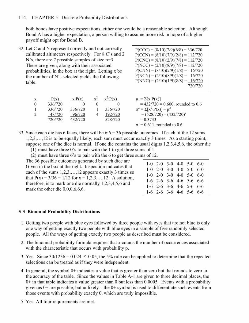
32. Let C and N represent correctly and not correctly calibrated altimeters respectively. For 8 C’s and 2 N’s, there are 7 possible samples of size n=3. These are given, along with their associated probabilities, in the box at the right. Letting x be the number of N’s selected yields the following table. x P(x) x·P(x) x2 x2·P(x) μ = Σ[x·P(x)] 0 336/720 0 0 0 = 432/720 = 0.600, rounded to 0.6 1 336/720 336/720 1 336/720 σ2 = Σ[x2·P(x)] – μ2 2 48/720 96/720 4 192/720 = (528/720) – (432/720)2 720/720 432/720 528/720 = 0.3733 σ = 0.611, rounded to 0.6

33. Since each die has 6 faces, there will be 6·6 = 36 possible outcomes. If each of the 12 sums 1,2,3,…,12 is to be equally likely, each sum must occur exactly 3 times. As a starting point, suppose one of the dice is normal. If one die contains the usual digits 1,2,3,4,5,6, the other die

(1) must have three 0’s to pair with the 1 to get three sums of 1. (2) must have three 6’s to pair with the 6 to get three sums of 12.

The 36 possible outcomes generated by such dice are Given in the box at the right. Inspection indicates that each of the sums 1,2,3,…,12 appears exactly 3 times so that P(x) = 3/36 = 1/12 for x = 1,2,3,…,12. A solution, therefore, is to mark one die normally 1,2,3,4,5,6 and mark the other die 0,0,0,6,6,6. 5-3 Binomial Probability Distributions 1. Getting two people with blue eyes followed by three people with eyes that are not blue is only one way of getting exactly two people with blue eyes in a sample of five randomly selected people. All the ways of getting exactly two people as described must be considered.

2. The binomial probability formula requires that x counts the number of occurrences associated with the characteristic that occurs with probability p.

3. Yes. Since 30/1236 = 0.024 ≤ 0.05, the 5% rule can be applied to determine that the repeated selections can be treated as if they were independent.

4. In general, the symbol 0+ indicates a value that is greater than zero but that rounds to zero to the accuracy of the table. Since the values in Table A-1 are given to three decimal places, the 0+ in that table indicates a value greater than 0 but less than 0.0005. Events with a probability given as 0+ are possible, but unlikely – the 0+ symbol is used to differentiate such events from those events with probability exactly 0, which are truly impossible.

5. Yes. All four requirements are met.

P(CCC) = (8/10)(7/9)(6/8) = 336/720 P(CCN) = (8/10)(7/9)(2/8) = 112/720 P(CNC) = (8/10)(2/9)(7/8) = 112/720 P(NCC) = (2/10)(8/9)(7/8) = 112/720 P(CNN) = (8/10)(2/9)(1/8) = 16/720 P(NCN) = (2/10)(8/9)(1/8) = 16/720 P(NNC) = (2/10)(1/9)(8/8) = 16/720 720/720

1-0 2-0 3-0 4-0 5-0 6-0 1-0 2-0 3-0 4-0 5-0 6-0 1-0 2-0 3-0 4-0 5-0 6-0 1-6 2-6 3-6 4-6 5-6 6-6 1-6 2-6 3-6 4-6 5-6 6-6 1-6 2-6 3-6 4-6 5-6 6-6

Binomial Probability Distributions SECTION 5-3 115 6. No. Requirement (3) is not met. There are more than two possible outcomes for the description of how one’s head feels.

7. No. Requirement (3) is not met. There are more than two possible outcomes for the ages of the parents.

8. Yes. All four requirements are met.

9. No. Requirements (2) and (4) are not met. Since 20/100 = 0.20 > 0.05, and the selections are done without replacement, the trials cannot be considered independent. The value p of obtaining a success changes from trial to trial as each selection without replacement changes the population from which the next selection is made.

10. No. Requirements (2) and (4) are not met. Since 15/50 = 0.30 > 0.05, and the selections are done without replacement, the trials cannot be considered independent. The value p of obtaining a success changes from trial to trial as each selection without replacement changes the population from which the next selection is made.

11. Yes. All four requirements are met. Since 500/2,800,000 = 0.00018 ≤ 0.05, the selections can considered to be independent – even though the they are made without replacement.

12. Yes. All four requirements are met. Since 200 statistics students are assumed to be less than 5% of the population of all statistics students, the selections can considered to be independent – even though they are made without replacement.

13. a. P(WWC) = P(W)·P(W)·P(C) = (4/5)(4/5)(1/5) = 16/125 = 0.128 b. There are three possible arrangements: WWC, WCW, CWW P(WWC) = P(W)·P(W)·P(C) = (4/5)(4/5)(1/5) = 16/125 P(WCW) = P(W)·P(C)·P(W) = (4/5)(1/5)(4/5) = 16/125 P(CWW) = P(C)·P(W)·P(W) = (1/5)(4/5)(4/5) = 16/125 c. P(exactly one correct) = P(WWC or WCW or CWW) = P(WWC) + P(WCW) + P(CWW) = 16/125 + 16/125 + 16/125 = 48/125 = 0.384

14. a. P(WWCCCC) = P(W)·P(W)·P(C)·P(C)·P(C)·P(C) = (3/4)(3/4)(1/4)(1/4)(1/4)(1/4) = 9/4096 = 0.00220 b. There are 6C2 = 6!/(4!2!) = 15 possible arrangements as listed below by columns. The probability for each arrangement will include the factor 3/4 two times and the factor 1/4 four times to give the result 9/4096 = 0.00220 of part (a). WWCCCC CWWCCC CCWWCC CCCWWC CCCCWW WCWCCC CWCWCC CCWCWC CCCWCW WCCWCC CWCCWC CCWCCW WCCCWC CWCCW WCCCCW c. P(exactly four correct) = P(WWCCCC or WCWCCC or…or CCCCWW) = P(WWCCCC) + P(WCWCCC) +…+ P(CCCCWW) = 9/4096 + 9/4096 +…+ 9/4096 = 15·(9/4096) = 135/4096 = 0.0330

15. From Table A-1 in the .30 column and the 2-1 row, P(x=1) = 0.420.

16. From Table A-1 in the .95 column and the 5-1 row, P(x=1) = 0+.

17. From Table A-1 in the .99 column and the 15-11 row, P(x=11) = 0+.

116 CHAPTER 5 Discrete Probability Distributions 18. From Table A-1 in the .60 column and the 14-4 row, P(x=4) = 0.014.

19. From Table A-1 in the .05 column and the 10-2 row, P(x=2) = 0.075.

20. From Table A-1 in the .70 column and the 12-12 row, P(x=12) = 0.014.

21. P(x) = n!(n-x)!x!

pxqn-x

P(x=10) = [12!/(2!10!)](0.75)10(0.25)2 = [66](0.0563)(0.0625) = 0.232

NOTE: The intermediate values 66, 0.0563, and 0.0625 are given in Exercise 21 to help those with an incorrect answer to identify the portion of the problem in which the mistake was made. In the future, only the value n!/[(n-x)!x!] will be given separately. In practice, all calculations can be done in one step on a calculator. You may choose (or be asked) to write down intermediate values for your own (or the instructor’s) benefit, but… • Never round off in the middle of a problem. • Do not write the values down on paper and then re-enter them in the calculator. • Use the memory to let the calculator remember with complete accuracy any intermediate values

that will be used in subsequent calculations. In addition, always make certain that n!/[(n-x)!x!] is a whole number and that the final answer is between 0 and 1.

22. P(x) = n!(n-x)!x!

pxqn-x

P(x=2) = [9!/(7!2!)](0.35)2(0.65)7 = [36](0.35)2(0.65)7 = 0.216

23. P(x) = n!(n-x)!x!

pxqn-x

P(x=4) = [20!/(16!4!)](0.15)4(0.85)16 = [4845](0.15)4(0.85)16 = 0.182

24. P(x) = n!(n-x)!x!

pxqn-x

P(x=13) = [15!/(2!13!)](1/3)13(2/3)2 = [105](1/3)13(2/3)2 = 0.0000293 25. P(x ≥ 1) = 1 – P(x=0) = 1 – 0.050328 = 0.949672, rounded to 0.0950 Yes, it is reasonable to expect that at least one group O donor will be obtained.

26. P(x ≥ 3) = P(x=3) + P(x=4) + P(x=5) = 0.275653 + 0.112767 + 0.018453 = 0.406873, rounded to 0.407 No, it is not very likely that at least 3 group O donors will be obtained. Since 0.407 > 0.05, getting at least 3 such donors would not be an unusual event – but it would not be considered very likely. NOTE: The answer to the question depends upon one’s interpretation of “very likely.” The answer is no if very likely is taken literally to mean “extremely likely.” The answer is yes if very likely is taken idiomatically to mean “reasonably possible.”

Binomial Probability Distributions SECTION 5-3 117 27. P(x=5) = 0.018453, rounded to 0.018 Yes. Since 0.018 ≤ 0.05, getting all 5 donors from group O would be considered unusual.

28. P(x ≤ 2) = P(x=0) + P(x=1) + P(x=2) = 0.050328 + 0.205889 + 0.336909 = 0.593126, rounded to 0.593

29. Let x = the number of consumers who recognize the Mrs. Fields brand name. binomial problem: n = 10 and p = 0.90, use Table A-1 a. P(x=9) = 0.387 b. P(x≠9) = 1 – P(x=9) = 1 – 0.387 = 0.613

30. Let x = the number of consumers who recognize the McDonald’s brand name. binomial problem: n = 15 and p = 0.95, use Table A-1 a. P(x=13) = 0.135 b. P(x≠13) = 1 – P(x=13) = 1 – 0.135 = 0.865

31. Let x = the number of people with brown eyes. binomial problem: n = 14 and p = 0.40, use Table A-1 P(x ≥ 12) = P(x=12) + P(x=13) + P(x=14) = 0.001 + 0+ + 0+ = 0.001 Yes. Since 0.001 ≤ 0.05, getting at least 12 persons with brown eyes would be unusual.

32. Let x = the number of delinquencies. binomial problem: n = 12 and p = 0.01, use Table A-1 P(x ≥ 1) = 1 – P(x=0) = 1 – 0.886 = 0.114 Yes. Since 0.114 > 0.05, it would not be unusual for at least one of the people to become delinquent. The bank should make plans for dealing with a delinquency.

33. Let x = the number of offspring peas with green pods. binomial problem: n = 10 and p = 0.75, use the binomial formula

P(x) = n!(n-x)!x!

pxqn-x

P(x ≥ 9) = P(x=9) + P(x=10) = [10!/(1!9!)](0.75)9(0.25)1 + [10!/(0!10!)](0.75)10(0.25)0 = [10](0.75)9(0.25)1 + [1](0.75)10(0.25)0 = 0.1877 + 0.0563 = 0.2440, rounded to 0.244 No. Since 0.244 > 0.05, getting at least 9 peas with green pods is not unusual.

34. Let x = the number of offspring peas with green pods. binomial problem: n=10 and p = 0.75, use the binomial formula

P(x) = n!(n-x)!x!

pxqn-x

P(x ≥ 1) = 1 – P(x=0) = 1 - [10!/(10!0!)](0.75)0(0.25)10 = 1 – [1](0.75)0(0.25)10 = 1 – 0.000000954 = 0.999999046, rounded to 0.999999 The usual rounded rule (to 3 significant digits) is not satisfactory in this case since applying

118 CHAPTER 5 Discrete Probability Distributions that rule would suggest that P(x ≥ 1) = 1.00, which is a certainty. In this case, 6 significant digits are necessary to differentiate the probability of this very likely event from the probability of an event that is a certainty.

35. Let x = the number of special program students who graduated. binomial problem: n = 10 and p = 0.94, use the binomial formula

P(x) = n!(n-x)!x!

pxqn-x

a. P(x ≥ 9) = P(x=9) + P(x=10) = [10!/(1!9!)](0.94)9(0.06)1 + [10!/(0!10!)](0.94)10(0.06)0 = [10](0.94)9(0.06)1 + [1](0.94)10(0.06)0 = 0.3438 + 0.5386 = 0.8824, rounded to 0.882 b. P(x=8) = [10!/(2!8!)](0.94)8(0.06)2 = [45](0.94)8(0.06)2 = 0.0988 P(x ≥ 8) = P(x=8) + P(x=9) + P(x=10) = 0.0988 + 0.3438 + 0.5386 = 0.9812 P(x ≤ 7) = 1 – P(x ≥ 8) = 1 – 0.9812 = 0.0188 Yes. Since P(x ≤ 7) = 0.0188 ≤ 0.05, getting only 7 that graduated would be unusual. NOTE: Remember that in situations involving multiple ordered outcomes, the unusualness of a particular outcome is generally determined by the probability of getting that outcome or a more extreme outcome.

36. Let x = the number of jackpots hit. [p = 1/2000 = 0.0005] binomial problem: n = 5 and p = 0.0005, use the binomial formula

P(x) = n!(n-x)!x!

pxqn-x

a. P(x=2) = [5!/(3!2!)](0.0005)2(0.9995)3 = [10](0.0005)2(0.9995)3 = 0.000002496 b. P(x ≥ 2) = 1 – P(x<2)

= 1 – {P(x=0) + P(x=1)} = 1 – {[5!/(5!0!)](0.0005)0(0.9995)5 + [5!/(4!1!)](0.0005)1(0.9995)4} = 1 – {[1](1)(0.9995)5 + [5](0.0005)(0.9995)4} = 1 – {.997502499 + 0.002495004} = 1 – {.99997503} = 0.000002497, rounded to 0.00000250 c. No. Since 0.000002497 ≤ 0.05, it would be unusual to hit two jackpots. If the machine is functioning as it is supposed to, either the guest is not telling the truth or an extremely rare event has occurred.

37. Let x = the number of households tuned to the NBC game if the stated share is correct. binomial problem: n = 20 and p = 0.22, use the binomial formula

P(x) = n!(n-x)!x!

pxqn-x

a. P(x=0) = [20!/(20!0!)](0.22)0(0.78)20 = [1](0.22)0(0.78)20 = 0.00695 b. P(x ≥ 1) = 1 – P(x=0)

= 1 – 0.00695 = 0.99305, rounded to 0.993 c. P(x=1) = [20!/(19!1!)](0.22)1(0.78)19 = [20](0.22)1(0.78)19 = 0.0392 P(at most 1) = P(x ≤ 1) = P(x=0) + P(x=1) = 0.0069 + 0.0392 = 0.0461

Binomial Probability Distributions SECTION 5-3 119 d. Yes. Since 0.0461 ≤ 0.05, getting at most one household tuned to the NBC game would be unusual. Either an unusual event has occurred or the 22% share value is incorrect.

38. Let x = the number with gonorrhea. binomial problem: n = 30 and p = 0.00114, use the binomial formula

P(x) = n!(n-x)!x!

pxqn-x

P(x=0) = [30!/(30!0!)](0.00114)0(0.99886)30 = [1](0.00114)0(0.99886)30 = 0.9664 P(sample tests positive) = P(x ≥ 1) = 1 – P(x=0) = 1 – 0.9664 = 0.0336 No. Since 0.0336 ≤ 0.05, having a sample test positive would be considered an unusual event. NOTE: This plan is very efficient. Suppose, for example, there were 3000 people to be tested. Only in 0.0336 = 3.36% of the groups would a retest need to be done for each of the 30 individuals. Those (0.0336)(100) ≈ 3 groups would generate (3)(30) = 90 retests. The total number of tests required would be 190 (the 100 original + the 90 retests), only 6.3% of the 3,000 tests that would have been required to test everyone individually.

39. Let x = the number who stayed less than one year. binomial problem: n = 15 and p = 0.36, use the binomial formula

P(x) = n!(n-x)!x!

pxqn-x

a. P(x=5) = [15!/(10!5!)](0.36)5(0.64)10 = [3003](0.36)5(0.64)10 = 0.209 b. The binomial distribution requires that the repeated selections be independent. Since these persons are selected from the original group of 320 without replacement, the repeated selections are not independent and the binomial distribution should not be used. In part (a), however, the sample size is 15/320 = 4.6% ≤ 5% of the population and the repeated samples may be treated as though they are independent. If the sample size is increased to 20, the sample is 20/320 = 6.25% > 5% of the population and the criteria for using independence to get an approximate probability is no longer met.

40. Let x = the number who said the most common mistake is not to know the company. binomial problem: n = 6 and p = 0.47, use the binomial formula

P(x) = n!(n-x)!x!

pxqn-x

a. P(x=3) = [6!/(3!3!)](0.47)3(0.53)3 = [20](0.47)3(0.53)3 = 0.309 b. The binomial distribution requires that the repeated selections be independent. Since these persons are selected from the original group of 150 without replacement, the repeated selections are not independent and the binomial distribution should not be used. In part (a), however, the sample size is 6/150 = 4.0% ≤ 5% of the population and the repeated samples may be treated as though they are independent. If the sample size is increased to 9, the sample is 9/150 = 6.0% > 5% of the population and the criteria for using independence to get an approximate probability is no longer met.

120 CHAPTER 5 Discrete Probability Distributions 41. Let x = the number of aspirin tablets that do not meet the specifications. binomial problem: n = 40 and p = 0.03, use the binomial formula

P(x) = n!(n-x)!x!

pxqn-x

P(accept shipment) = P(x=0) + P(x=1) = [40!/(40!0!)](0.03)0(0.97)40 + [40!/(39!1!)](0.03)1(0.97)39 = [1](0.03)0(0.97)40 + [40](0.03)1(0.97)39 = 0.2957 + 0.3658 = 0.6615, rounded to 0.662 Approximately 2/3 of such shipments will be accepted.

42. Let x = the number of booked passengers that show up for the flight. binomial problem: n = 24 and p = 1 – 0.0995 = 0.9005, use the binomial formula

P(x) = n!(n-x)!x!

pxqn-x

P(not enough seats) = P(x=23) + P(x=24) = [24!/(1!23!)](0.9005)23(0.0995)1 + [24!/(0!24!)](0.9005)24(0.0995)0 = [24](0.9005)23(0.0995)1 + [1](0.9005)40(0.0995)0 = 0.2144 + 0.0808 = 0.2952, rounded to 0.295 No. Since 0.295 > 0.05, such an event would not be unusual. The probability is high enough so that overbooking is a real concern.

43. Let x = the number of females hired if there is no discrimination. binomial problem: n = 24 and p = 0.50, use the binomial formula

P(x) = n!(n-x)!x!

pxqn-x

P(x ≤ 3) = P(x=0) + P(x=1) + P(x=2) + P(x=3) = [24!/(24!0!)](0.5)0(0.5)24 + [24!/(23!1!)](0.5)1(0.5)23

+ [24!/(22!2!)](0.5)2(0.05)22 + [24!/(21!3!)](0.5)3(0.5)21 = [1](0.5)0(0.5)24 + [24](0.5)1(0.5)23 + [276](0.5)2(0.5)22 + [2024](0.5)3(0.05)21 = 0.00000006 + 0.00000143 + 0.00001645 + 0.00012063 = 0. 00013857, rounded to 0.000139 Yes. Since 0.000139 ≤ 0.05, such an event would be unusual. Either a very unusual event has occurred or there is gender discrimination.

44. Let x = the number of defective pens if there has been no change in the rate. binomial problem: n = 60 and p = 0.06, use the binomial formula

P(x) = n!(n-x)!x!

pxqn-x

a. P(x=1) = [60!/(59!1!)](0.5)0(0.5)24

= [60](0.06)1(0.94)59 = 0.0935 b. P(x=0) = [60!/(60!0!)](0.06)0(0.94)60

= [1](0.06)0(0.94)60 = 0.0244 c. In situations involving multiple ordered outcomes, the unusualness of a particular outcome is generally determined by the probability of getting that outcome or a more extreme outcome. In this instance the appropriate probability is P(x ≤ 1) = P(x=0) + P(x=1) = 0.0935 + 0.0244 = 0.1179, rounded to 0.118 d. Since 0.118 > 0.05, the observed outcome would not be considered unusual under the old rate. There is not sufficient evidence to conclude that the modified procedure is better.

Binomial Probability Distributions SECTION 5-3 121 45. Let x = the number of peas with green pods binomial problem: n = 580 and p = 0.75, use the binomial formula

P(x) = n!(n-x)!x!

pxqn-x

P(x=428) = [580!/(152!428!)](0.75)428(0.25)152

= 0.0301231, rounded to 0.0301 Since 0.0301 ≤ 0.05, this particular result might be considered unusual – but so would any of the 581 possible individual outcomes. In situations involving multiple ordered outcomes, the unusualness of a particular outcome is generally determined by the probability of getting that outcome or a more extreme outcome. In this instance the appropriate probability is P(x ≤ 428) = 0.264956, rounded to 0.265 Since 0.265 > 0.05, the obtained result is not considered unusual – and there is no suggestion that Mendel’s probability value of 0.75 is wrong. NOTE: The large factorials required are beyond the capabilities of most calculators. The above answers [P(x=428) = 0.0301231, and P(x ≤ 428) = 0.264956] were obtained using the Minitab software package.

46. Let x = the number of persons tested to find the first blood donor with blood type O negative. geometric problem: p = 0.06 and x = 12, use the geometric formula P(x) = p(1-p)x-1 P(x=7) = (0.06)(0.94)11 = 0.0304

47. Let x = the number of winners selected. hypergeometric problem: A=6 (winners), B=53 (losers) and n=6 (selections)

( )

A! B! (A+B)!P(x) = ÷(A-x)!x! (B-n+x)! n-x ! (A+B-n)!n!

⋅

a. P(x=6) = [6!/(0!6!)]·[53!/(53!0!)] ÷ [59!/(53!6!)] = [1]·[1] ÷ [45,057,474] = 0.0000000222 b. P(x=5) = [6!/(1!5!)]·[53!/(52!1!)] ÷ [59!/(53!6!)] = [6]·[53] ÷ [45,057,474] = 0.00000706 c. P(x=3) = [6!/(3!3!)]·[53!/(50!3!)] ÷ [59!/(53!6!)] = [20]·[23,426] ÷ [45,057,474] = 0.0104 d. P(x=0) = [6!/(6!0!)]·[53!/(47!6!)] ÷ [59!/(53!6!)] = [1]·[22,957,480] ÷ [45,057,474] = 0.510 NOTE: This formula is actually [ACx]·[BCn-x] ÷ [A+BCn] and follows directly from the methods of section 4-7.

48. Extending the pattern to cover six types of outcomes, where Σx = n and Σp = 1, n=20 and p1=p2=p3=p4=p5=p6=1/6 and x1=5, x2=4, x3=3, x4=2, x5=3, x6=3 use the multinomial formula P(x1,x2,x3,x4,x5,x6) = [n!/(x1!x2!x3!x4!x5!x6!)](p1)x1(p2)x2(p3)x3(p4)x4(p5)x5(p6)x6 = [20!/(5!4!3!2!3!3!)](1/6)5(1/6)4(1/6)3(1/6)2(1/6)3(1/6)3 = [1,955,457,504,030]·(1/6)20 = 0.000535

122 CHAPTER 5 Discrete Probability Distributions 5-4 Mean, Variance, and Standard Deviation for the Binomial Distribution 1. Yes. By definition q = 1−p. The two expressions represent the same numerical quantity, and they may be used interchangeably

2. The standard deviation cannot be a negative number. The smallest possible standard deviation is zero, indicating that all the values are identical. The given standard deviation is not correct. Since the Excel software would never give a negative standard deviation, the user presumably was using the software’s spreadsheet capabilities and input the wrong formula or the wrong value for n, μ, Σx, or Σx2.

3. Using the exact formula, σ2 = npq = 1236(0.05)(0.95) = 58.71, rounded to 58.7 people2. Using the rounded value given for σ, σ2 = (σ)2 = (7.7)2 = 59.29, rounded to 59.3 people2.

4. The binomial distribution does not apply. Since the students are selected without replacement, repeated selections are not independent and the probability of getting a female changes for each selection. The formulas in this section do not apply.

5. μ = np = (50)(0.2) = 10.0 σ2 = npq = (50)(0.2)(0.8) = 8; σ = 2.828, rounded to 2.8 minimum usual value = μ – 2σ = 10 – 2(2.828) = 4.3 maximum usual value = μ + 2σ = 10 + 2(2.828) = 15.7

6. μ = np = (152)(0.5) = 76.0 σ2 = npq = (152)(0.5)(0.5) = 38; σ = 6.164, rounded to 6.2 minimum usual value = μ – 2σ = 76.0 – 2(6.164) = 63.7 maximum usual value = μ + 2σ = 76.0 + 2(6.164) = 88.3

7. μ = np = (300)(0.48) = 144.0 σ2 = npq = (300)(0.48)(0.52) = 74.88; σ = 8.653, rounded to 8.7 minimum usual value = μ – 2σ = 144.0 – 2(8.653) = 126.7 maximum usual value = μ + 2σ = 144.0 + 2(8.653) = 161.3

8. μ = np = (1236)(0.14) = 173.04. rounded to 173.0 σ2 = npq = (1236)(0.14)(0.86) = 148.8144; σ = 12.199, rounded to 12.2 minimum usual value = μ – 2σ = 173.04 – 2(12.199) = 148.6 maximum usual value = μ + 2σ = 173.04 + 2(12.199) = 197.4

9. Let x = the number of correct answers. binomial problem: n = 75 and p = 0.5 a. μ = np = (75)(0.5) = 37.5 σ2 = npq = (75)(0.5)(0.5) = 18.75; σ = 4.330, rounded to 4.3 b. Unusual values are those outside μ ± 2σ 37.5 ± 2(4.330) 37.5 ± 8.7 28.8 to 46.2 [using rounded values, 28.9 to 46.1] No. Since 45 is within the above limits, it would not be unusual for a student to pass by getting at least 45 correct answers.

10. Let x = the number of correct answers. binomial problem: n = 100 and p = 0.2 a. μ = np = (100)(0.2) = 20.0 σ2 = npq = (100)(0.2)(0.8) = 16.00; σ = 4.0

Mean, Variance, and Standard Deviation for the Binomial Distribution SECTION 5-4 123 b. Unusual values are those outside μ ± 2σ 20.0 ± 2(4.0) 20.0 ± 8.0 12.0 to 28.0 Yes. Since 60 is not within the above limits, it would be unusual for a student to pass by getting at least 60 correct answers.

11. Let x = the number of green M&M’s. binomial problem: n = 100 and p = 0.16 a. μ = np = (100)(0.16) = 16.0 σ2 = npq = (100)(0.16)(0.84) = 13.44; σ = 3.666, rounded to 3.7 b. Unusual values are those outside μ ± 2σ 16.0 ± 2(3.666) 16.0 ± 7.3 8.7 to 23.3 [using rounded values, 8.6 to 23.4] No. Since 19 is within the above limits, it would not be unusual for 100 M&M’s to include 19 green ones. This is not evidence that the claimed rate of 16% is wrong.

12. Let x = the number of blue M&M’s. binomial problem: n = 100 and p = 0.16 a. μ = np = (100)(0.24) = 24.0 σ2 = npq = (100)(0.24)(0.76) = 18.24; σ = 4.271, rounded to 4.3 b. Unusual values are those outside μ ± 2σ 24.0 ± 2(4.271) 24.0 ± 8.5 15.5 to 32.5 [using rounded values, 15.4 to 32.6] No. Since 27 is within the above limits, it would not be unusual for 100 M&M’s to include 27 blue ones. This is not evidence that the claimed rate of 24% is wrong.

13. Let x = the number of baby girls. binomial problem: n = 574 and p = 0.5 a. μ = np = (574)(0.5) = 287.0 σ2 = npq = (574)(0.5)(0.5) = 143.5; σ = 11.979, rounded to 12.0 b. Unusual values are those outside μ ± 2σ 287.0 ± 2(11.979) 287.0 ± 24.0 263.0 to 311.0 Yes. Since 525 is not within the above limits, it would be unusual for 574 births to include 525 girls. The results suggest that the gender selection method is effective.

14. Let x = the number of baby boys. binomial problem: n = 152 and p = 0.5 a. μ = np = (152)(0.5) = 76.0 σ2 = npq = (152)(0.5)(0.5) = 38.0; σ = 6.164, rounded to 6.2 b. Unusual values are those outside μ ± 2σ 76.0 ± 2(6.164) 76.0 ± 12.3 63.7 to 86.3 [using rounded values, 63.6 to 88.4] Yes. Since 127 is not within the above limits, it would be unusual for 152 births to include 127 girls. The results suggest that the gender selection method is effective.

124 CHAPTER 5 Discrete Probability Distributions 15. Let x = the number who stay at their first job less than two years. binomial problem: n = 320 and p = 0.5 a. μ = np = (320)(0.5) = 160.0 σ2 = npq = (320)(0.5)(0.5) = 80.0; σ = 8.944, rounded to 8.9 b. Unusual values are those outside μ ± 2σ 160.0 ± 2(8.944) 160.0 ± 17.9 142.1 to 177.9 [using rounded values, 142.2 to 177.8] c. x = (0.78)(320) = 250 [actually 248,249,250,251 all round to 78%] Since 250 is not within the above limits, it would be unusual for 320 graduates to include 250 persons who stayed at their first job less than two years if the true proportion were 50%. Since 250 is greater than the above limits, the true proportion is most likely greater than 50%. The result suggests that the headline is justified. d. The statement suggests that the 320 participants were a voluntary response sample, and so the results might not be representative of the target population.

16. Let x = the number of plants with short stems. binomial problem: n = 1064 and p = 0.25 a. μ = np = (1064)(0.25) = 266.0 σ2 = npq = (1064)(0.25)(0.75) = 199.5; σ = 14.124, rounded to 14.1 b. Unusual values are those outside μ ± 2σ 266.0 ± 2(14.124) 266.0 ± 28.2 237.8 to 294.2 No. Since 277 is within the above limits, it would not be not unusual for 1064 offspring plants to include 277 with short stems. The results give no evidence that Mendel’s theory is not correct.

17. Let x = the number of persons who voted. binomial problem: n = 1002 and p = 0.61 a. μ = np = (1002)(0.61) = 611.22 σ2 = npq = (1002)(0.61)(0.39) = 238.3758; σ = 15.439, rounded to 15.4 b. Unusual values are those outside μ ± 2σ 611.22 ± 2(15.439) 611.22 ± 30.88 580.3 to 642.1 [using rounded values, 580.4 to 642.0] No. Since 701 is not within the above limits, it would be unusual for 1002 potential voters to include 701 who actually voted. The results are not consistent with the actual voter turnout and suggest that those polled may not be telling the truth. c. No. It appears that asking persons how they acted may not yield accurate results.

18. Let x = the number of persons with cancer of the brain or nervous system. binomial problem: n = 420,095 and p = 0.000340 a. μ = np = (420095)(0.000340) = 142.8 σ2 = npq = (420095)(0.000340)(0.999660) = 142.784; σ = 11.949, rounded to 11.9 b. Unusual values are those outside μ ± 2σ 142.8 ± 2(11.949) 142.8 ± 23.9 118.9 to 166.7 [using rounded σ, 119.0 to 166.6] No. Since 135 is within the above limits, it is not an unusual result. c. These results do not provide evidence that cell phone use increases the risk of such cancers.

Mean, Variance, and Standard Deviation for the Binomial Distribution SECTION 5-4 125 19. Let x = the number of persons receiving the drug who experience nausea. binomial problem: n = 821 and p = 0.0124 a. μ = np = (821)(0.0124) = 10.18 σ2 = npq = (821)(0.0124)(0.9876) = 10.0542; σ = 3.171, rounded to 3.2 b. Unusual values are those outside μ ± 2σ 10.18 ± 2(3.171) 10.18 ± 6.34 3.8 to 16.5 [using rounded values, 3.8 to 16.6] Yes. Since 30 is not within the above limits, it is an unusual result. c. Perhaps. The results suggest that Chantix does increase the likelihood of experiencing nausea, but at 30/821 = 3.65% that probability is still relatively low.

20. Let x = the number of times the therapist correctly identifies the selected hand. binomial problem: n = 280 and p = 0.5 a. μ = np = (280)(0.5) = 140.0 σ2 = npq = (280)(0.5)(0.5) = 70.0; σ = 8.367, rounded to 8.4 b. Unusual values are those outside μ ± 2σ 140.0 ± 2(8.367) 140.0 ± 16.7 123.3 to 156.7 [using rounded values, 123.2 to 156.8] Yes. Since 123 is not within the above limits, it is an unusual result – but one that has fewer, and not more, correct identifications than expected by chance. The results suggest that touch therapists do not have the ability to select correctly by sensing an energy field. The results may suggest that any energy field the therapists sense is diminished by the nearness of another human, and that is why they sensed an energy field more often than chance would predict over the hand where there was no human presence. It may also be that Emily Rosa happens to be a rare individual with a “negative” energy field. It would be interesting to see if further studies, using both Emily and another experimenter, also get this unexpected result.

21. Refer to the Exercise 47 in Section 5-3 and the NOTE at the end of the problem. Let x = the number of females selected. P(x) = [10Cx][30C12-x]/[40C12] P(0) = [10C0][30C12]/[40C12] = 1·86493225/5586853480 = 86,493,225/5,586,853,480 P(1) = [10C1][30C11]/[40C12] = 10·54627300/5586853480 = 546,273,000/5,586,853,480 P(2) = [10C2][30C10]/[40C12] = 45·30045015/5586853480 = 1,352,025,675/5,586,853,480 P(3) = [10C3] [30C9]/[40C12] = 120·14307150/5586853480 = 1,716,858,000/5,586,853,480 P(4) = [10C4] [30C8]/[40C12] = 210·5852925/ 5586853480 = 1,229,114,250/5,586,853,480 P(5) = [10C5] [30C7]/[40C12] = 252·2035800/ 5586853480 = 513,021,600/5,586,853,480 P(6) = [10C6] [30C6]/[40C12] = 210·593775/5586853480 = 124,692,750/5,586,853,480 P(7) = [10C7] [30C5]/[40C12] = 120·142506/5586853480 = 17,100,720/5,586,853,480 P(8) = [10C8] [30C4]/[40C12] = 45·27405/5586853480 = 1,233,225/5,586,853,480 P(9) = [10C9] [30C3]/[40C12] = 10·4060/5586853480 = 40,600/5,586,853,480 P(10) = [10C10] [30C2]/[40C12] = 1·435/ 5586853480 = 435/5,586,853,480 5,586,853,440/5,586,853,480

There are 40C12 = 5,586,853,440 total ways that a group of 12 persons can be selected from a class of 40. The number of females in each group can range from x=0 to x=10. The probability of each of those x values is given above – in fraction form, to indicate the exact numbers of ways involved for each type of group.

126 CHAPTER 5 Discrete Probability Distributions The following table, with the probabilities converted to decimal form, follows the methods of this chapter to calculate the mean and standard deviation of the probability distribution. The given table is a probability distribution since 0 ≤ P(x) ≤ 1 for each x and ΣP(x)=1. x P(x) x·P(x) x2 x2·P(x) μ = Σ[x·P(x)] 0 0.0154815 0 0 0 = 3 1 0.0977782 0.0977783 1 0.0977783 σ2 = Σ[x2·P(x)] – μ2 2 0.2420012 0.4840026 4 0.9680051 = 10.6153846 – 32 3 0.3073032 0.9219096 9 2.7657289 = 1.6153846 4 0.2200011 0.8800046 16 3.5200186 σ = 1.2709, rounded to 1.3 5 0.0918266 0.4591329 25 2.2956643 6 0.0223190 0.1339137 36 0.8034825 7 0.0030608 0.0214262 49 0.1499834 8 0.0002207 0.0017659 64 0.0141272 9 0.0000073 0.0000654 81 0.0005886 10 0.0000001 0.0000008 100 0.0000078 1.0000000 3.0000000 10.6153846

22. Let x = the number of edible pizzas binomial problem: n is unknown and p=0.8. We want P(x ≥ 5) ≥ 0.99. for n=5, P(x ≥ 5) = P(x=5) = 0.328 = 0.328 for n=6, P(x ≥ 5) = P(x=5) + P(x=6) = 0.393 + 0.262 = 0.655 for n=7, P(x ≥ 5) = P(x=5) + P(x=6) + P(x=7) = 0.275 + 0.367 + 0. 210 = 0.852 for n=8, P(x ≥ 5) = P(x=5) + P(x=6) + P(x=7) + P(x=8) = 0.147 + 0.294 + 0.336 + 0.168 = 0.945 for n=9, P(x ≥ 5) = P(x=5) + P(x=6) + P(x=7) + P(x=8) + P(x=9) = 0.066 + 0.176 + 0.302 + 0.302 + 0.134 = 0.980 for n=10, P(x ≥ 5) = P(x=5) + P(x=6) + P(x=7) + P(x=8) + P(x=9) + P(x=10) = 0.026 + 0.088 + 0.201 + 0.302 + 0.268 + 0.107 = 0.992 The minimum number of pizzas necessary to be at least 99% sure that there will be 5 edible pizzas available is n=10. NOTE: Because mathematical formulation of this problem involves complicated algebra that does not promote better understanding of the concepts involved, use a trial-and-error approach and Table A-1. This procedure may not be the most efficient, but it is easy to follow and promotes better understanding of the concepts involved. 5-5 Poisson Probability Distributions 1. The Poisson distribution describes the numbers of occurrences, over some defined interval, of independent random events that are uniformly distributed over that interval.

2. Ignoring leap years, μ = 126/365 = 0.345 σ = μ = 0.345 = 0.588 σ2 = μ = 0.345

3. The probability 4.82x10-64 is so small that for all practical purposes it is equal to zero.

Poisson Probability Distributions SECTION 5-5 127 4. The experiment may be described as follows. Let x = the number of 2’s that occur binomial problem: n = 6 and p = 1/6 This not a Poisson problem with the defined interval being 6 rolls of the die. In a Poisson problem there is no limit on the value for x, the number of occurrences of the event. But in this experiment the number of occurrences cannot be more than 6. The binomial probability 0.335 is the correct one.

5. P(x) = μxe-μ/x! with μ = 2 P(x=3) = (2)3(e-2)/3! = (8)(0.1353)/6 = 0.180

NOTE: The intermediate values 8, 0.1353 and 6 are given in exercise #5 to help students who are unable to get the correct answer and need to identify where they are going wrong. In practice, the answer can be obtained on a calculator in one step without writing down intermediate values. If you write down intermediate values (for your sake or the instructor’s), DO NOT USE ROUNDED INTERMEDIATE VALUES IN SUBSEQUENT CALCULATIONS. IF NECESSARY, USE THE MEMORY TO STORE INTERMEDIATE VALUES WITH COMPLETE ACCURACY. Intermediate values given in subsequent Poisson problems are for instructional purposes only.

6 P(x) = μxe-μ/x! with μ = 0.3 P(x=1) = (0.3)1(e-0.3)/1! = (0.3)(0.7408)/1 = 0.222

7. P(x) = μxe-μ/x! with μ = 0.75 P(x=3) = (0.75)3(e-0.75)/3! = (0.4219)(0.4624)/6 = 0.0332

8. P(x) = μxe-μ/x! with μ = 1/6 P(x=3) = (1/6)0(e-1/6)/0! = (1)(0.8465)/1 = 0.846

IMPORTANT NOTE: In the problems that follow, store the unrounded value for μ for use in all Poisson calculations.

9. Let x = the number of motor vehicle deaths per day. Poisson problem: use P(x) = μxe-μ/x! a. Ignoring leap years, μ = 35.4/365 = 0.0970 b. P(x=0) = (0.0970)0(e-0.0970)/0! = (1)(0.9076)/1 = 0.907568 P(x=1) = (0.0970)1(e-0.0970)/1! = (0.0970)(0.9076)/1 = 0.088022 P(x=2) = (0.0970)2(e-0.0970)/2! = (0.0094)(0.9076)/2 = 0.004268 P(x ≤ 2) = P(x=0) + P(x=1) + P(x=2) = 0.907568 + 0.088022 + 0.004268 = 0.999859 P(x>2) = 1 – P(x ≤ 2) = 1 – 0.999859 = 0.000141 c. Yes. Since 0.000141 ≤ 0.05, having more than 2 motor vehicle deaths on the same day is unusual.

128 CHAPTER 5 Discrete Probability Distributions 10. Let x = the number of low birth weight babies born per day. Poisson problem: use P(x) = μxe-μ/x! a. Ignoring leap years, μ = 210.0/365 = 0.575 b. P(x=0) = (0.575)0(e-0.575)/0! = (1)(0.5625)/1 = 0.5625 P(x=1) = (0.575)1(e-0.575)/1! = (0.5625)(0.9076)/1 = 0.3236 P(x ≤ 2) = P(x=0) + P(x=1) + P(x=2) = 0.5625 + 0.3236 = 0.8861 P(x>1) = 1 – P(x ≤ 1) = 1 – 0.8861 = 0.1139, rounded to 0.114 c. No. Since 0.114 > 0.05, having more than 1 low weight baby born on the same day is not unusual.

11. Let x = the number of atoms lost per day. Poisson problem: use P(x) = μxe-μ/x! a. The number of atoms lost is 1,000,000 – 997,287 = 22,713. μ = 22,713/365 = 62.2 b. P(x=50) = (62.2)50(e-62.2)/50! = 0.0155

NOTE: Exercises 12 and 13 compare actual results to predictions by the Poisson probability distribution. The comparison can be made either by changing the actual frequencies to relative frequencies (by dividing by n = Σf) and comparing them to the predicted Poisson probabilities, or by changing the Poisson probabilities to predicted frequencies (by multiplying by n = Σf) and comparing them to the actual frequencies. We use the first approach, but the choice is arbitrary.

12. Let x = the number of horse-kick deaths per corps per year. Poisson problem: μ = 196/280 = 0.70, use P(x) = μxe-μ/x! a. P(x=0) = (0.70)0(e-0.70)/0! = (1)(0.4966)/1 = 0.4966 b. P(x=1) = (0.70)1(e-0.70)/1! = (0.70)(0.4966)/1 = 0.3476 c. P(x=2) = (0.70)2(e-0.070)/2! = (0.4900)(0.4966)/2 = 0.1217 d. P(x=3) = (0.70)3(e-0.070)/3! = (0.3430)(0.4966)/6 = 0.0284 e. P(x=4) = (0.70)4(e-0.070)/4! = (0.2401)(0.4966)/24 = 0.00497 The following table compares the actual relative frequencies to the Poisson probabilities. x f r.f. P(x) . 0 144 0.5143 0.4966 NOTE: r.f. = f/Σf = f/280 1 91 0.3250 0.3476 2 32 0.1143 0.1217 3 11 0.0393 0.0284 4 2 0.0071 0.0050 5 or more 0 0.0000 0.0007 (by subtraction) 280 1.0000 1.0000 Yes. The agreement between the actual relative frequencies and the probabilities predicted by the Poisson formula is very good.

13. Let x = the number of homicides per day. Poisson problem: μ = 116/365 = 0.3178, use P(x) = μxe-μ/x! a. P(x=0) = (0.3178)0(e-0.3178)/0! = (1)(0.7277)/1 = 0.7277 b. P(x=1) = (0.3178)1(e-0.3178)/1! = (0.3178)(0.7277)/1 = 0.2313 c. P(x=2) = (0.3178)2(e-0.3178)/2! = (0.1010)(0.7277)/2 = 0.0368 d. P(x=3) = (0.3178)3(e-0.3178)/3! = (0.0321)(0.7277)/6 = 0.00389

Poisson Probability Distributions SECTION 5-5 129 e. P(x=4) = (0.3178)4(e-0.3178)/4! = (0.0102)(0.7277)/24 = 0.000309 The following table compares the actual relative frequencies to the Poisson probabilities. x f r.f. P(x) . 0 268 0.7342 0.7277 NOTE: r.f. = f/Σf = f/365 1 79 0.2164 0.2313 2 17 0.0466 0.0368 3 1 0.0027 0.0038 4 or more 0 0.0000 0.0004 (by subtraction) 365 1.0000 1.0000 The agreement is very good.

14. Let x = the number of neuroblastoma cases. binomial problem: n = 12,429 and p = 0.000011 a. μ = np = (12429)(0.000011) = 0.136719 b. Since n = 12,429 ≥ 100 and np = 0.136710 ≤ 10, use the Poisson approximation to the binomial: μ = 0.136719 and P(x) = μxe-μ/x! P(x=0) = (0.136719)0 (e-0.136719)/0! = (1)(0.8722)/1 = 0.872215 P(x=1) = (0.136719)1 (e-0.136719)/1! = (0.136719)(0.8722)/1 = 0.119248 P(x=0 or x=1) = P(x=0) + P(x=1) = 0.872215 + 0.119248 = 0.99146 c. P(x>1) = 1 – P(x ≤ 1) = 1 – 0.99146 = 0.00854 d. No. Since P(x ≥ 4) < P(x>1) = 0.00854, getting four such cases by chance alone is an unusual event. Either a very rare event has occurred or, more likely, there appears to be some cancer-causing factor at work.. NOTE: Parts (b)-(d) can be answered using the exact binomial distribution as follows.

P(x) = n!(n-x)!x!

pxqn-x

P(x=0) = [12429!/(12429!0!)](0.000011)0(0.999989)12429 = [1](0.000011)0(0.999989)12429 = 0.872215 P(x=1) = [12429!/(12428!1!)](0.000011)1(0.999989)12428 = [12429](0.000011)0(0.999989)12429 = 0.119250 P(x=0 or x=1) = P(x=0) + P(x=1) = 0.872215 + 0.119250 = 0.99146 To the usual level of accuracy, the answers agree.

15. Let x = the number of such women who die during the year. binomial problem: n = 700 and p = 1 – 0.9968 = 0.0032 a. μ = np = (700)(0.0032) = 2.24 b. Since n = 700 ≥ 100 and np = 2.24 ≤ 10, use the Poisson approximation to the binomial: μ = 2.24 and P(x) = μxe-μ/x! P(x=0) = (2.24)0 (e-2.24)/0! = (1)(0.1065)/1 = 0.10645 P(x=1) = (2.24)1 (e-2.24)/1! = (2.24)(0.1065)/1 = 0.23847 P(x=2) = (2.24)2 (e-2.24)/2! = (2.24)2(0.1065)/2 = 0.26708 P(x=3) = (2.24)3 (e-2.24)/3! = (2.24)3(0.1065)/6 = 0.19942 P(x<4) = P(x=0) + P(x=1) + P(x=2) + P(x=3) = 0.10645 + 0.23847 + 0.26708 + 0.19942 = 0.811 No. The probability of making a profit is relatively high, but the company is not “almost sure” to make a profit.

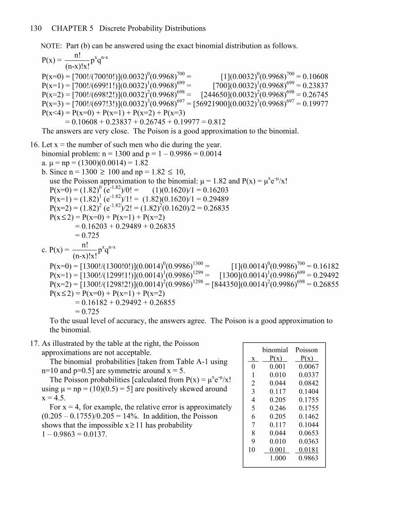
130 CHAPTER 5 Discrete Probability Distributions NOTE: Part (b) can be answered using the exact binomial distribution as follows.

P(x) = n!(n-x)!x!

pxqn-x

P(x=0) = [700!/(700!0!)](0.0032)0(0.9968)700 = [1](0.0032)0(0.9968)700 = 0.10608 P(x=1) = [700!/(699!1!)](0.0032)1(0.9968)699 = [700](0.0032)1(0.9968)699 = 0.23837 P(x=2) = [700!/(698!2!)](0.0032)2(0.9968)698 = [244650](0.0032)2(0.9968)698 = 0.26745 P(x=3) = [700!/(697!3!)](0.0032)3(0.9968)697 = [56921900](0.0032)3(0.9968)697 = 0.19977 P(x<4) = P(x=0) + P(x=1) + P(x=2) + P(x=3) = 0.10608 + 0.23837 + 0.26745 + 0.19977 = 0.812 The answers are very close. The Poison is a good approximation to the binomial.

16. Let x = the number of such men who die during the year. binomial problem: n = 1300 and p = 1 – 0.9986 = 0.0014 a. μ = np = (1300)(0.0014) = 1.82 b. Since n = 1300 ≥ 100 and np = 1.82 ≤ 10, use the Poisson approximation to the binomial: μ = 1.82 and P(x) = μxe-μ/x! P(x=0) = (1.82)0 (e-1.82)/0! = (1)(0.1620)/1 = 0.16203 P(x=1) = (1.82)1 (e-1.82)/1! = (1.82)(0.1620)/1 = 0.29489 P(x=2) = (1.82)2 (e-1.82)/2! = (1.82)2(0.1620)/2 = 0.26835 P(x ≤ 2) = P(x=0) + P(x=1) + P(x=2) = 0.16203 + 0.29489 + 0.26835 = 0.725

c. P(x) = n!(n-x)!x!

pxqn-x

P(x=0) = [1300!/(1300!0!)](0.0014)0(0.9986)1300 = [1](0.0014)0(0.9986)700 = 0.16182 P(x=1) = [1300!/(1299!1!)](0.0014)1(0.9986)1299 = [1300](0.0014)1(0.9986)699 = 0.29492 P(x=2) = [1300!/(1298!2!)](0.0014)2(0.9986)1298 = [844350](0.0014)2(0.9986)698 = 0.26855 P(x ≤ 2) = P(x=0) + P(x=1) + P(x=2) = 0.16182 + 0.29492 + 0.26855 = 0.725 To the usual level of accuracy, the answers agree. The Poison is a good approximation to the binomial.

17. As illustrated by the table at the right, the Poisson approximations are not acceptable. The binomial probabilities [taken from Table A-1 using n=10 and p=0.5] are symmetric around x = 5. The Poisson probabilities [calculated from P(x) = μxe-μ/x! using μ = np = (10)(0.5) = 5] are positively skewed around x = 4.5. For x = 4, for example, the relative error is approximately (0.205 – 0.1755)/0.205 = 14%. In addition, the Poisson shows that the impossible x ≥ 11 has probability 1 – 0.9863 = 0.0137.

binomial Poisson x P(x) P(x) . 0 0.001 0.0067 1 0.010 0.0337 2 0.044 0.0842 3 0.117 0.1404 4 0.205 0.1755 5 0.246 0.1755 6 0.205 0.1462 7 0.117 0.1044 8 0.044 0.0653 9 0.010 0.0363 10 0.001 0.0181. 1.000 0.9863

Statistical Literacy and Critical Thinking 131 Statistical Literacy and Critical Thinking 1. A random variable is a variable that has a single value, determined by chance, for each outcome of a procedure. Yes, a discrete random variable can have an infinite number of possible values – e.g., the number of coin tosses required to get the first head can be 1,2,3,4,…

2. A discrete random variable has a countable number of possible values – i.e., its possible values are either finite, or they can by placed in a well-defined 1-to-1 correspondence with the positive integers. A continuous random variable has an infinite number of possible values that are associated with measurements on a continuous scale – i.e., a scale in which there are generally no gaps or interruptions between the possible values.

3. In a binomial probability distribution, there are exactly two possible outcomes: p is the probability of one of the outcomes (usually called “success”), and q is the probability of the other outcome (usually called “failure”). Since the two outcomes are mutually exclusive and exhaustive, p+q = 1. This means that q = 1–p and that p = 1–q.

4. No. Other named discrete probability distributions identified in the exercises are the geometric distribution (Section 5-3, Exercise 46) and the hypergeometric distribution (Section 5-3, Exercise 47). There are also general unnamed discrete probability distributions (e.g., Section 5-2, Exercise 11. Chapter Quick Quiz 1. No. Since P(x=0)+P(x=1) = 0.8+0.8 = 1.6 violates the requirement that ΣP(x) = 1, the given scenario does not define a probability distribution.

2. As shown by the table at the right, μ = Σ[x·P(x)] = 0.7.

3. The scenario describes a binomial probability distribution with n = 400 and p = 0.5. μ = np = (400)(0.5) = 200

4. The scenario describes a binomial probability distribution with n = 400 and p = 0.5. σ2 = npq = (400)(0.5)(0.5) = 100; σ = 10

5. Yes. Any value more than two standard deviations from the mean is generally considered unusual, and 35 is (35-20.0)/4.0 = 3.75 standard deviations from the mean.

6. Yes. The scenario describes a binomial probability distribution with n = 5 and p = 0.2 A check of the given P(x) values indicates they were generated by the binomial formula

P(x) = n!(n-x)!x!

pxqn-x.

7. P(x ≥ 1) = 1 – P(x=0) = 1 – 0.4096 = 0.5904

8. P(x ≤ 4) = P(x=0) + P(x=1) + P(x=2) + P(x=3) + P(x=4) = 0.4096 + 0.4096 + 0.1536 + 0.0256 + 0.0016 = 0.9984 P(x=5) = 1 – P(x ≤ 4) = 1 – 0.9984 = 0.0016

9. P(x=2 or x=3) = P(x=2) + P(x=3) = 0.1536 + 0.0256 = 0.1792

10. Yes. Since P(x=5) = 0.0016 ≤ 0.05, getting all five answers correct by random guessing would be an unusual event.

x P(x) x·P(x) 0 0.3 0.0 1 0.7 0.7 1.0 0.7

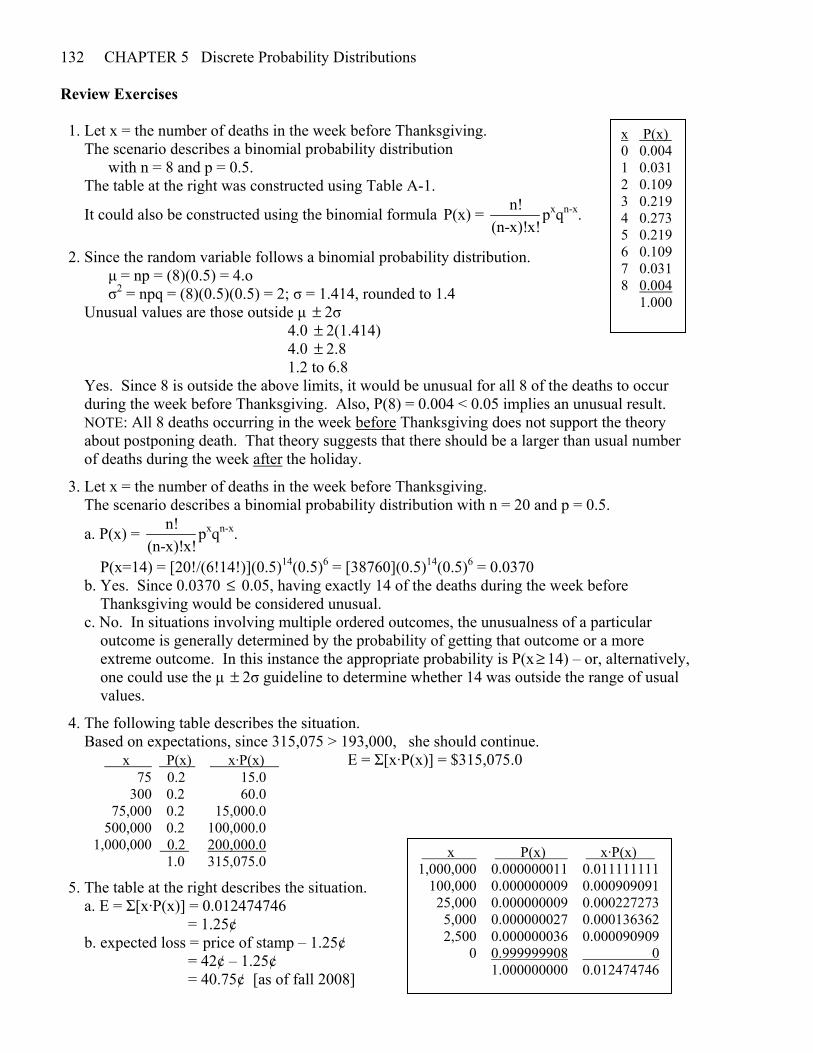
132 CHAPTER 5 Discrete Probability Distributions Review Exercises 1. Let x = the number of deaths in the week before Thanksgiving. The scenario describes a binomial probability distribution with n = 8 and p = 0.5. The table at the right was constructed using Table A-1.

It could also be constructed using the binomial formula P(x) = n!(n-x)!x!

pxqn-x.

2. Since the random variable follows a binomial probability distribution. μ = np = (8)(0.5) = 4.o σ2 = npq = (8)(0.5)(0.5) = 2; σ = 1.414, rounded to 1.4 Unusual values are those outside μ ± 2σ 4.0 ± 2(1.414) 4.0 ± 2.8 1.2 to 6.8 Yes. Since 8 is outside the above limits, it would be unusual for all 8 of the deaths to occur during the week before Thanksgiving. Also, P(8) = 0.004 < 0.05 implies an unusual result. NOTE: All 8 deaths occurring in the week before Thanksgiving does not support the theory about postponing death. That theory suggests that there should be a larger than usual number of deaths during the week after the holiday.

3. Let x = the number of deaths in the week before Thanksgiving. The scenario describes a binomial probability distribution with n = 20 and p = 0.5.

a. P(x) = n!(n-x)!x!

pxqn-x.

P(x=14) = [20!/(6!14!)](0.5)14(0.5)6 = [38760](0.5)14(0.5)6 = 0.0370 b. Yes. Since 0.0370 ≤ 0.05, having exactly 14 of the deaths during the week before Thanksgiving would be considered unusual. c. No. In situations involving multiple ordered outcomes, the unusualness of a particular outcome is generally determined by the probability of getting that outcome or a more extreme outcome. In this instance the appropriate probability is P(x ≥ 14) – or, alternatively, one could use the μ ± 2σ guideline to determine whether 14 was outside the range of usual values.

4. The following table describes the situation. Based on expectations, since 315,075 > 193,000, she should continue. x P(x) x·P(x) E = Σ[x·P(x)] = $315,075.0 75 0.2 15.0 300 0.2 60.0 75,000 0.2 15,000.0 500,000 0.2 100,000.0 1,000,000 0.2 200,000.0 1.0 315,075.0

5. The table at the right describes the situation. a. E = Σ[x·P(x)] = 0.012474746 = 1.25¢ b. expected loss = price of stamp – 1.25¢ = 42¢ – 1.25¢ = 40.75¢ [as of fall 2008]

x P(x) . 0 0.004 1 0.031 2 0.109 3 0.219 4 0.273 5 0.219 6 0.109 7 0.031 8 0.004 1.000

x P(x) x·P(x) . 1,000,000 0.000000011 0.011111111 100,000 0.000000009 0.000909091 25,000 0.000000009 0.000227273 5,000 0.000000027 0.000136362 2,500 0.000000036 0.000090909 0 0.999999908 0 1.000000000 0.012474746

Review Exercises 133 No. From a purely financial point of view, it is not worth entering this contest. NOTE: The biggest winner in the sweepstakes appears to be the USPS. Based on the probabilities of winning, it appears that the company expects about 100,000,000 entries. At 42¢ per entry, the sweepstakes would generate 42 million dollars of entry postage alone!

6. No. Since P(x=0)+P(x=1)+P(x=2)+P(x=3)+P(x=4) = 0.0016+0.0250+0.1432+0.3892+0.4096 = 0.9686 violates the requirement that ΣP(x) = 1, the given scenario does not describe a probability distribution.

7. a. There are 10 possible values [0,1,2,3,4,5,6,7,8,9] for each digit. There are 10·10·10·10 = 10,000 ways to select the 4 digits. Since only one selection wins, P(W) = 1/10,000 = 0.0001 b. Refer to the table in part (e). The first two columns give the desired probability distribution. c. The expected number of wins in 365 tries is 365(.0001) = 0.0365. d. The scenario describes a binomial probability distribution with n = 365 and p = 0.0001.

P(x) = n!(n-x)!x!

pxqn-x.

P(x=1) = [365!/(364!1!)](0.0001)1(0.9999)364 = [365](0.0001)1(0.9999)364 = 0.0352 e. Refer to the table. E = Σ[x·P(x)] = −0.5000 = − 50¢.

8. a. Let x = the number fired for not getting along with others. binomial problem: n = 5 and p = 0.17, use the binomial formula

P(x) = n!(n-x)!x!

pxqn-x

P(x ≥ 4) = P(x=4) + P(x=5) = [5!/(1!4!)](0.17)4(0.83)1 + [5!/(0!5!)](0.17)5(0.83)0

= [5](0.17)4(0.83)1 + [1](0.17)5(0.83)0 = 0.003466 + 0.000142 = 0. 003608, rounded to 0.00361 b. Yes. Since 0.00361 ≤ 0.05, such an event would be unusual for a typical company operating with p = 0.17. Either a rare event has occurred or, more likely, this company is different.

9. Let x = the number of checks with leading digit 1. binomial problem: n = 784 and p = 0.301, use the binomial formula a. The expected number is the mean, μ = np = (784)(0.301) = 236.0 b. For the binomial distribution, μ = np = (784)(0.301) = 236.0 σ2 = npq = (784)(0.301)(0.699) = 164.9528; σ = 12.843, rounded to 12.8 c. Usual values are those within μ ± 2σ 236.0 ± 2(12.843) 236.0 ± 25.7 210.3 to 261.7 [using rounded values, 210.4 to 261.6] d. Yes. Since 0 is so far outside the above limits, that would be very strong evidence that the checks are different (and likely fraudulent).

10. Let x = the number of bombs per region Poison problem: use P(x) = μxe-μ/x! a. μ = 535/576 = 0.9288 b. P(x=0) = (0.9288)0e-0,9288/0! = (1)(0.3950)/1 = 0.395 c. We expect (576)(0.395) = 227.53, or about 228, regions not to be hit. d. The actual result of 229 is very close to the result predicted by the Poison formula.

x P(x) x·P(x) . −1 0.9999 −0.9999 4999 0.0001 0.4999 1.0000 −0.5000

134 CHAPTER 5 Discrete Probability Distributions Cumulative Review Exercises 1. Arranged in order, the values are: 115.00 134.83 142.94 188.00 217.60 summary statistics: n = 5 Σx = 798.37 Σx2 = 134529.7325

a. x = (Σx)/n = 798.37/5 = $159.674

b. x = x3 = $142.94

c. R = xn – x1 = 217.60 – 115.00 = $102.60

d. s = $41.985 [the square root of the answer given in part e]

e. s2 = [n(Σx2) – (Σx)2]/[n(n-1)] = [5(134529.7325) – (798.37)2]/[5(4)] = 35254.0056/20 = 1762.700 dollars2

f. Usual values are those within x ± 2s 159.674 ± 2(41.9845) 159.674 ± 83.969 75.705 to 243.643 [using rounded values, 75.704 to 243.644]

g. No. Since all of the sample values are within the above limits, none of them is unusual.

h. Ratio, since differences are meaningful and there is a meaningful zero.

i. Discrete, since checks must be written in whole numbers of cents.

j. Convenience, since they were selected because they happened to be close at hand.

k. Since the sample was a random sample, the sample mean of the n items observed should be a good estimate of the population mean of all N items. The estimate for the population total is N x = (134)(159.674) = $21,396.316. 2. Let x = the number of companies that test employees for substance abuse. binomial problem: n = 10 and p = 0.80, use Table A-1

a. P(x=5) = 0.026

b. P(x ≥ 5) = P(x=5) + P(x=6) + P(x=7) + P(x=8) + P(x=9) + P(x=10) = 0.026 + 0.088 + 0.201 + 0.302 + 0.268 + 0.107 = 0.992

c. For the binomial distribution, μ = np = (10)(0.80) = 8.0 σ2 = npq = (10)(0.80)(0.20) = 1.60; σ = 1.2649, rounded to 1.3

d. Usual values are those within μ ± 2σ 8.0 ± 2(1.2649) 8.0 ± 2.5 5.5 to 10.5 [using rounded values, 5.4 to 10.6]

Cumulative Review Exercises 135 3. Let x = the number of HIV cases. binomial problem: n = 150 and p = 0.10, use the binomial formula

P(x) = n!(n-x)!x!

pxqn-x.

a. μ = np = (150)(0.10) = 15.0 σ2 = npq = (150)(0.10)(0.90) = 13.5; σ = 3.674, rounded to 3.7

b. Usual values are those within μ ± 2σ 15.0 ± 2(3.674) 15.0 ± 7.3 7.7 to 22.3 [using rounded values, 7.6 to 22.4] No. Since 12 is within the above limits, it is not an unusually low result. There is not sufficient evidence to suggest that the program is effective in lowering the 10% rate. 4. Let S = the selected passenger was one who survived.

a. P(S) = 706/2223 = 0.318

b. P(S1 and S2) = P(S1)·P(S2|S1) = (706/2223)(705/2222) = 0.101

c. P( S ) = 1 – P(S) = 1 – 706/2223 = 1517/2223 P( 1S and 2S ) = P( 1S )·P( 2S | 1S ) = (1517/2223)(1516/2222) = 0.466 5. No. The correct value is the weighted mean of the 50 state means, with the population of each state as the weight. If the means are not weighted, then small population states count equal with large population states – and a small population state with unusually high or low per capita consumption has undue influence and incorrectly affects the national mean as much as a large population state.