4-1

Chapter 4 Quantum Spookiness

As we have seen in the previous chapters, many aspects of quantum mechanics run counter to our physical intuition, which is formed from our experience living in the classical world. The probabilistic nature of quantum mechanics does not agree with the certainty of the classical world—we have no doubt that the sun will rise tomorrow. Moreover, the disturbance of a quantum mechanical system through the action of measurement makes us part of the system, rather than an independent observer. These issues and others make us wonder what is really going on in the quantum world. As quantum mechanics was being developed in the early 20th century, many of the world's greatest physicists debated the "true meaning" of quantum mechanics. They often developed gedanken experiments or thought experiments to illustrate their ideas. Some of these gedanken experiments have now actually been performed and some are still being pursued.

In this chapter, we present a few of the gedanken and real experiments that demonstrate the spookiness of quantum mechanics. We present enough details to give a flavor of the spookiness and provide references for further readings on these topics at the end of the chapter.

4.1 Einstein-Podolsky-Rosen Paradox

Albert Einstein was never comfortable with quantum mechanics. He is famously quoted as saying "Gott würfelt nicht" or "God does not play dice," to express his displeasure with the probabilistic nature of quantum mechanics. But his opposition to quantum mechanics ran deeper than that. He felt that properties of physical objects have an objective reality independent of their measurement, much as Erwin felt that his socks were black or white, or long or short, independent of his pulling them out of the drawer. In quantum mechanics, we cannot say that a particle whose spin is measured to be up had that property before the measurement. It may well have been in a superposition state. Moreover, we can only know one spin component of a particle, because measurement of one component disturbs our knowledge of the other components. Because of these apparent deficiencies, Einstein believed that quantum mechanics was an incomplete

description of reality. In 1935, Einstein, Boris Podolsky, and Nathan Rosen published a paper

presenting a gedanken experiment designed to expose the shortcomings of quantum mechanics. The EPR Paradox (Einstein-Podolsky-Rosen) tries to paint quantum mechanics into a corner and expose the "absurd" behavior of the theory. The essence of the argument is that if you believe that measurements on two widely separated particles cannot influence each other, then the quantum mechanics of an ingeniously prepared two-particle system leads you to conclude that the physical properties of each particle are really there—they are elements of reality in the authors’ words.

Chap. 4 Quantum Spookiness

8/10/10

4-2

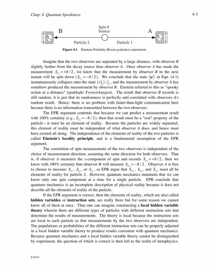
The experimental situation is depicted in Fig. 4.1 (this version of the EPR experiment is due to David Bohm and has been updated by N. David Mermin). An unstable particle with spin 0 decays into two spin-1/2 particles, which by conservation of angular momentum must have opposite spin components and by conservation of linear momentum must travel in opposite directions. For example, a neutral pi meson decays into an electron and a positron: ! 0

" e#!+!e

+ . Observers A and B are on opposite sides of the decaying particle and each has a Stern-Gerlach apparatus to measure the spin component of the particle headed in its direction. Whenever one observer measures spin up along a given direction, then the other observer measures spin down along that same direction. The quantum state of this two-particle system is

! =1

2+

1"

2!"!! "

1+

2( ) , (4.1)

where the subscripts label the particles and the relative minus sign ensures that this is a spin-0 state (as we'll discover in Chap. 11). The use of a product of kets (e.g., +

1!

2)

is required here to describe the two-particle system (HW). The kets and operators for the two particles are independent, so, for example, operators act only on their own kets

S1z+

1!

2= S

1z+

1( ) !

2= +!

2+

1!

2 (4.2)

and inner products behave as

1+

2!( ) +

1!

2( ) = 1

+ +1

( ) 2! !

2( ) = 1 (4.3)

The reason that the state vector in Eqn. (4.1) is a spin-0 state will become clear in Chapter 11.

As shown in Fig. 4.1, observer A measures the spin component of particle 1 and observer B measures the spin component of particle 2. The probability that observer A measures particle 1 to be spin up is 50% and the probability for spin down is 50%. The 50-50 split is the same for observer B. For a large ensemble of decays, each observer records a random sequence of spin up and spin down results, with a 50/50 ratio. But, because of the correlation between the spin components of the two particles, if observer A measures spin up (i.e.,

S1z= +! / 2 ), then we can predict with 100% certainty that the

result of observer B’s measurement will be spin down ( S2z= !! / 2 ). The result is that

even though each observer records a random sequence of ups and downs, the two sets of results are perfectly anti-correlated. The state ! in Eqn. (4.1) that produces this strange mixture of random and correlated measurement results is known as an entangled

state. The spins of the two particles are entangled with each other and produce this perfect correlation between the measurements of observer A and observer B.

Chap. 4 Quantum Spookiness

8/10/10

4-3

ABParticle 1Particle 2

Spin 0 Source

S1zS2z

Figure 4.1 Einstein-Podolsky-Rosen gedanken experiment.

Imagine that the two observers are separated by a large distance, with observer B

slightly farther from the decay source than observer A. Once observer A has made the measurement

S1z= +! / 2 , we know that the measurement by observer B in the next

instant will be spin down ( S2z= !! / 2 ). We conclude that the state ! in Eqn. (4.1)

instantaneously collapses onto the state +1!

2, and the measurement by observer A has

somehow produced the measurement by observer B. Einstein referred to this as "spooky action at a distance" (spukhafte Fernwirkungen). The result that observer B records is still random, it is just that its randomness is perfectly anti-correlated with observers A's random result. Hence, there is no problem with faster-than-light communication here because there is no information transmitted between the two observers.

The EPR argument contends that because we can predict a measurement result with 100% certainty (e.g.,

S2z= !! / 2 ), then that result must be a "real" property of the

particle—it must be an element of reality. Because the particles are widely separated, this element of reality must be independent of what observer A does, and hence must have existed all along. The independence of the elements of reality of the two particles is called Einstein's locality principle, and is a fundamental assumption of the EPR argument.

The correlation of spin measurements of the two observers is independent of the choice of measurement direction, assuming the same direction for both observers. That is, if observer A measures the x-component of spin and records

S1x= +! / 2 , then we

know with 100% certainty that observer B will measure S2x= !! / 2 . Observer A is free

to choose to measure S1x

, S1y , or S

1z, so EPR argue that S

2x, S

2y , and S2z

must all be elements of reality for particle 2. However, quantum mechanics maintains that we can know only one spin component at a time for a single particle. EPR conclude that quantum mechanics is an incomplete description of physical reality because it does not describe all the elements of reality of the particle.

If the EPR argument is correct, then the elements of reality, which are also called hidden variables or instruction sets, are really there but for some reason we cannot know all of them at once. Thus one can imagine constructing a local hidden variable

theory wherein there are different types of particles with different instruction sets that determine the results of measurements. The theory is local because the instruction sets are local to each particle so that measurements by the two observers are independent. The populations or probabilities of the different instruction sets can be properly adjusted in a local hidden variable theory to produce results consistent with quantum mechanics. Because quantum mechanics and a local hidden variable theory cannot be distinguished by experiment, the question of which is correct is then left to the realm of metaphysics.

Chap. 4 Quantum Spookiness

8/10/10

4-4

For many years, this was what many physicists believed. After all, it doesn't seem unreasonable to believe that there are things we cannot know!

However, in 1964, John Bell showed that the hidden variables that we cannot know cannot even be there! Bell showed that there are specific measurements that can be made to distinguish between a local hidden variable theory and quantum mechanics. The results of these quantum mechanics experiments are not compatible with any local hidden variable theory. Bell derived a very general relation, but we present a specific one here for simplicity.

Bell's argument relies on observers A and B making measurements along a set of different directions. Consider three directions a, b, c in a plane as shown in Fig. 4.2, each 120° from any of the other two. Each observer makes measurements of the spin projection along one of these three directions, chosen randomly. Any single observer's result can be only spin up or spin down along that direction, but we record the results independent of the direction of the Stern-Gerlach analyzers, so we denote one observer's result simply as + or –, without noting the axis of measurement. The results of the pair of measurements from one correlated pair of particles (i.e., one decay from the source) are denoted + –, for example, which means observer A recorded a + and observer B recorded a –. There are only four possible system results: ++, + – , – + , or – –. Even more simply, we classify the results as are either the same, ++ or – –, or opposite, + – or – +.

A local hidden variable theory needs a set of instructions for each particle that specifies ahead of time what the results of measurements along the three directions a, b, c will be. For example, the instruction set (a+, b+, c+) means that a measurement along any one of the three directions will produce a spin up result. For the entangled state of the system give by Eqn. (4.1) measurements by the two observers along the same direction can yield only the results + – or – +. To reproduce this aspect of the data, a local hidden variable theory would need the 8 instruction sets shown in Table 4.1. For example, the instruction set (a+, b!, c+) for particle 1 must be paired with the set (a!, b+, c!) for particle 2 in order to produce the proper correlations of the entangled state. Beyond that requirement, we allow the proponent of the local hidden variable theory freedom to adjust the populations N

i (or probabilities) of the different instruction

sets as needed to make sure that the hidden variable theory agrees with the quantum mechanical results.

AB

a

c b

a

c b Particle 1Particle 2

Spin 0 Source

Figure 4.2 Measurement of spin components along three directions as proposed by Bell.

Chap. 4 Quantum Spookiness

8/10/10

4-5

Now use the instruction sets (i.e., the local hidden variable theory) to calculate the probability that the results of the spin component measurements are the same (!

same= !

+++ !

!!) and the probability that the results are opposite (

!opp

= !+!+ !

+!),

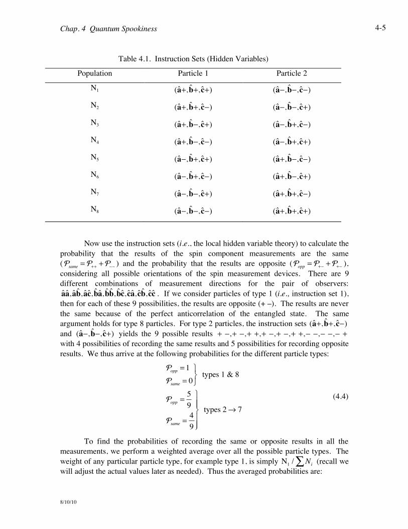
considering all possible orientations of the spin measurement devices. There are 9 different combinations of measurement directions for the pair of observers: aa, ab, ac, ba, bb, bc, ca, cb, cc . If we consider particles of type 1 (i.e., instruction set 1), then for each of these 9 possibilities, the results are opposite (+ –). The results are never the same because of the perfect anticorrelation of the entangled state. The same argument holds for type 8 particles. For type 2 particles, the instruction sets (a+, b+, c!) and (a!, b!, c+) yields the 9 possible results +!!,+!!,+!+,+!!,+!!,+!+,!!!,!!!,!!+ with 4 possibilities of recording the same results and 5 possibilities for recording opposite results. We thus arrive at the following probabilities for the different particle types:

!opp

= 1

!same

= 0

!"#

types 1!&!8

!opp

=5

9

!same

=4

9

!

"$$

#$$

types 2% 7

(4.4)

To find the probabilities of recording the same or opposite results in all the measurements, we perform a weighted average over all the possible particle types. The weight of any particular particle type, for example type 1, is simply N

1/ N

i! (recall we will adjust the actual values later as needed). Thus the averaged probabilities are:

Table 4.1. Instruction Sets (Hidden Variables)

Population Particle 1 Particle 2

N1 (a+, b+, c+) (a!, b!, c!)

N2 (a+, b+, c!) (a!, b!, c+)

N3 (a+, b!, c+) (a!, b+, c!)

N4 (a+, b!, c!) (a!, b+, c+)

N5 (a!, b+, c+) (a+, b!, c!)

N6 (a!, b+, c!) (a+, b!, c+)

N7 (a!, b!, c+) (a+, b+, c!)

N8 (a!, b!, c!) (a+, b+, c+)

Chap. 4 Quantum Spookiness

8/10/10

4-6

!same

=1

Ni

i

!4

9N2+ N

3+ N

4+ N

5+ N

6+ N

7( ) "4

9

!opp

=1

Ni

i

!N1+ N

8+5

9N2+ N

3+ N

4+ N

5+ N

6+ N

7( )#$%

&'()5

9

, (4.5)

where the inequalities follow because the sum of all the weights for the different particle types must sum to one. In summary, we can adjust the populations all we want but that will always produce probabilities of the same or opposite measurements that are bound by the above inequalities. That is what is meant by a Bell inequality.

What does quantum mechanics predict for these probabilities? For this system of 2 spin-1/2 particles, we can calculate the probabilities using the concepts from the previous chapters. Assume that observer A records a "+" along some direction (of the three) and define that direction as the z-axis (no law against that). Observer B measures along a direction n at some angle ! with respect to the z-axis. The probability that observer A records a "+" along the z-axis and observer B records a "+" along the n direction is

!++

=1+ !

2 n+( ) !

2

, (4.6)

Substituting the entangled state ! and the direction eigenstate +n

gives

!++

=1+ cos

!2!2+ !!+!!e

" i#sin

!2!2"$

%&'()

1

2+

1"

2!"!! "

1+

2( )

2

= 1

2cos

!2!2+ !!+!!e

" i#sin

!2!2"$

%&'()

"2

( )2

=1

2sin

2!2

, (4.7)

The same result is obtained for the probability that observer A records a "–" along the z-axis and observer B records a "–" along the n direction. Hence the result for same measurements is

!same

= !+++ !

!!= sin

2"

2, (4.8)

The probability that observer B records a "–" along the direction n , when A records a "+" is

Chap. 4 Quantum Spookiness

8/10/10

4-7

!+! = 1

+ !2 n

!( ) "2

=1+ sin

#2!2+ !!!!!e! i$ cos

#2!2!%

&'()*

1

2+

1!

2!!!! !

1+

2( )

2

= 1

2sin

#2!2+ !!!!!e! i$ cos

#2!2!%

&'()*

!2

( )2

=1

2cos

2#2

, (4.9)

and the probability for opposite results is

!opp

= !+!+ !

!+= cos

2"

2. (4.10)

The angle ! between the measurement directions of observers A and B is 0° in 1/3 of the measurements and 120° in 2/3 of the measurements, so the average probabilities are

!same

=1

3!sin

20°

2+2

3!sin

2120°

2=1

3!0 +

2

3!3

4=1

2

!opp

=1

3!cos

20°

2+2

3!cos

2120°

2=1

3!1+

2

3!1

4=1

2

, (4.11)

These predictions of quantum mechanics are inconsistent with the range of possibilities that we derived for local hidden variable theories in Eqn. (4.5). Because these probabilities can be measured, we can do experiments to test whether local hidden variable theories are possible. The results of experiments performed on systems that produce entangled quantum states have consistently agreed with quantum mechanics and hence exclude the possibility of local hidden variable theories. We are forced to conclude that quantum mechanics is an inherently nonlocal theory.

The EPR paradox also raises issues regarding the collapse of the quantum state and how a measurement by A can instantaneously alter the quantum state at B. However, there is no information transmitted instantaneously and so there is no violation of relativity. What observer B measures is not affected by any measurements that A makes. The two observers notice only when they get together and compare results that some of the measurements (along the same axes) are correlated.

The entangled states of the EPR paradox have truly nonclassical behavior and so appear spooky to our classically trained minds. But when you are given lemons, make lemonade. Modern quantum researchers are now using the spookiness of the entangled states to enable new technologies that take advantage of the way that quantum mechanics stores information in these correlated systems. Quantum computers, quantum communication, and quantum information processing in general are active areas of research and promise to enable a new revolution in information technology.

Chap. 4 Quantum Spookiness

8/10/10

4-8

4.2 Schrödinger Cat Paradox

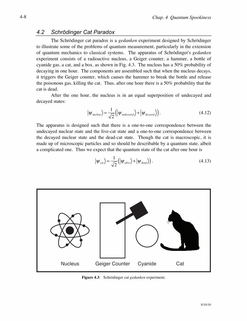
The Schrödinger cat paradox is a gedanken experiment designed by Schrödinger to illustrate some of the problems of quantum measurement, particularly in the extension of quantum mechanics to classical systems. The apparatus of Schrödinger's gedanken experiment consists of a radioactive nucleus, a Geiger counter, a hammer, a bottle of cyanide gas, a cat, and a box, as shown in Fig. 4.3. The nucleus has a 50% probability of decaying in one hour. The components are assembled such that when the nucleus decays, it triggers the Geiger counter, which causes the hammer to break the bottle and release the poisonous gas, killing the cat. Thus, after one hour there is a 50% probability that the cat is dead.

After the one hour, the nucleus is in an equal superposition of undecayed and decayed states:

! nucleus =1

2! undecayed + ! decayed( ) . (4.12)

The apparatus is designed such that there is a one-to-one correspondence between the undecayed nuclear state and the live-cat state and a one-to-one correspondence between the decayed nuclear state and the dead-cat state. Though the cat is macroscopic, it is made up of microscopic particles and so should be describable by a quantum state, albeit a complicated one. Thus we expect that the quantum state of the cat after one hour is

!cat

=1

2!

alive+ !

dead( ) . (4.13)

Nucleus Geiger Counter Cyanide Cat

Figure 4.3: Schrödinger cat gedanken experiment.

Chap. 4 Quantum Spookiness

8/10/10

4-9

Both quantum calculations and classical reasoning would predict 50/50 probabilities of observing an alive or a dead cat when we open the box. However, quantum mechanics would lead us to believe that the cat was neither dead nor alive before we opened the box, but rather was in a superposition of states and the quantum state collapses to the alive state !

alive or dead state !

dead only when we open the box

and make the measurement by observing the cat. But our classical experiences clearly run counter to this. We would say that the cat really was dead or alive, we just did not know it yet. (Imagine that the cat is wearing a cyanide sensitive watch—the time will tell us when the cat was killed if it is dead!)

Why are we so troubled by a cat in a superposition state? After all, we have just finished three chapters of electrons in superposition states! What is so inherently different about cats and electrons? Experiment 4 that we studied in Chapters 1 and 2 provides a clue. The superposition state in that experiment exhibits a clear interference effect that relies on the coherent phase relationship between the two parts of the superposition state vector for the spin-! particle. No one has ever observed such an interference effect with cats, so our gut feeling that cats and electrons are different appears justified.

The main issues raised by the Schrödinger cat gedanken experiment are (1) Can we describe macroscopic states quantum mechanically? and (2) What causes the collapse of the wave function?

The Copenhagen interpretation of quantum mechanics championed by Bohr and Heisenberg maintains that there is a boundary between the classical and quantum worlds. We describe microscopic systems (the nucleus) with quantum states and macroscopic systems (the cat, or even the Geiger counter) with classical rules. The measurement apparatus causes the quantum state to collapse and to produce the single classical or meter result. The actual mechanism for the collapse of the wave function is not specified in the Copenhagen interpretation, and where to draw the line between the classical and the quantum world is not clear. Others have argued that the human consciousness is responsible for collapsing the wave function, while some have argued that there is no collapse, just bifurcation into alternate, independent universes. Many of these different points of view are untestable experimentally and thus raise more metaphysical than physical questions.

These debates about the interpretation of quantum mechanics arise when we use words, which are based on our classical experiences, to describe the quantum world. The mathematics of quantum mechanics is clear and allows us to calculate precisely. No one is disagreeing about the probability that the cat will live or die. The disagreement is all about "what it really means!" To steer us toward the clear mathematics, Richard Feynman admonished us to "Shut up and calculate!" Two physicists who disagree on the words they use to describe a quantum mechanical experiment generally agree on the mathematical description of the results.

Recent advances in experimental techniques have allowed experiments to probe the boundary between the classical and quantum worlds and address the quantum measurement issues raised by the Schrödinger cat paradox. The coupling between the

Chap. 4 Quantum Spookiness

8/10/10

4-10

microscopic nucleus and the macroscopic cat is representative of a quantum measurement whereby a classical meter (the cat) provides a clear and unambiguous measurement of the state of the quantum system (the nucleus). In this case, the two possible states of the nucleus (undecayed or decayed) are measured by the two possible positions on the meter (cat alive or cat dead). The quantum mechanical description of this complete system is the entangled state

! system =1

2! undecayed ! alive !+!! decayed ! dead( ) . (4.14)

The main issue to be addressed by experiment is whether Eqn. (4.14) is the proper quantum mechanical description of the system. That is, is the system in a coherent quantum mechanical superposition, as described by Eqn. (4.14), or is the system in a 50/50 statistical mixed state of the two possibilities? As discussed above, we can distinguish these two cases by looking for interference between the two states of the system.

To build a Schrödinger cat experiment, researchers use a two-state atom as the quantum system and an electromagnetic field in a cavity as the classical meter (or cat). The atom can either be in the ground g or excited e state. The cavity is engineered to be in a coherent state ! described by the complex number ! , whose magnitude is equal to the square root of the average number of photons in the cavity. For large ! , the coherent state is equivalent to a classical electromagnetic field, but for small ! , the field appears more quantum mechanical. The beauty of this experiment is that the experimenters can tune the value of ! between these limits to study the region between the microscopic and macroscopic descriptions of the meter (cat). In this intermediate range, the meter is a mesoscopic system.

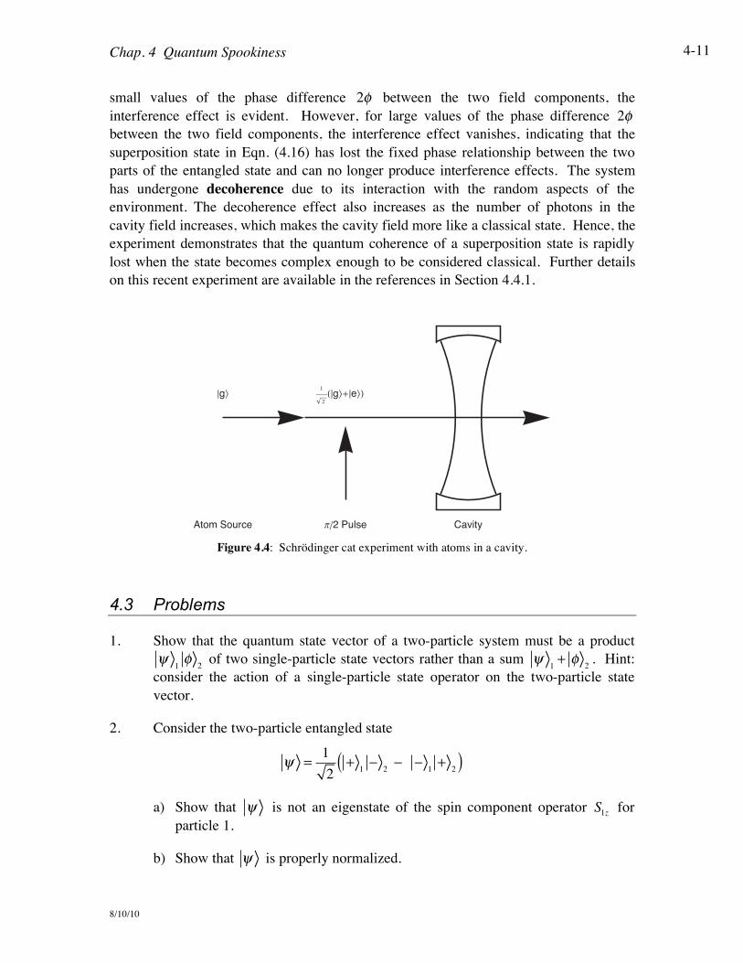
Atoms travel through the cavity and disturb the electromagnetic field in the cavity. Each atom is modeled as having an index of refraction that alters the phase of the electromagnetic field. The system is engineered such that the ground and excited atomic states produce opposite phase shifts ±! . Before the atom enters the cavity it undergoes a ! -pulse that places it in an equal superposition of ground and excited states

!atom

=1

2e !+! g( ) . (4.15)

as shown in Fig. 4.4. Each component of this superposition produces a different phase shift in the cavity field such that after the atom passes through the cavity, the atom-cavity system is in the entangled state

!atom+cavity

=1

2e "ei# !+! g "e$ i#( ) . (4.16)

that mirrors the Schrödinger cat state in Eqn. (4.14). The state of the cavity field is probed by sending a second atom into the cavity and looking for interference effects in the atom that are produced by the two components of the field. In this experiment, the two field states are classically distinguishable, akin to the alive and dead cat states. For

Chap. 4 Quantum Spookiness

8/10/10

4-11

small values of the phase difference 2! between the two field components, the interference effect is evident. However, for large values of the phase difference 2! between the two field components, the interference effect vanishes, indicating that the superposition state in Eqn. (4.16) has lost the fixed phase relationship between the two parts of the entangled state and can no longer produce interference effects. The system has undergone decoherence due to its interaction with the random aspects of the environment. The decoherence effect also increases as the number of photons in the cavity field increases, which makes the cavity field more like a classical state. Hence, the experiment demonstrates that the quantum coherence of a superposition state is rapidly lost when the state becomes complex enough to be considered classical. Further details on this recent experiment are available in the references in Section 4.4.1.

†g\ H†g\+†e\L

Atom Source p/2 Pulse Cavity

1

2

Figure 4.4: Schrödinger cat experiment with atoms in a cavity.

4.3 Problems

1. Show that the quantum state vector of a two-particle system must be a product !

1"

2 of two single-particle state vectors rather than a sum !

1+ "

2. Hint:

consider the action of a single-particle state operator on the two-particle state vector.

2. Consider the two-particle entangled state

! =1

2+

1"

2!"!! "

1+

2( )

a) Show that ! is not an eigenstate of the spin component operator S1z

for particle 1.

b) Show that ! is properly normalized.

Chap. 4 Quantum Spookiness

8/10/10

4-12

3. Consider the two-particle entangled state

! =1

2+

1"

2!"!! "

1+

2( )

Show that the probability of observer A measuring particle 1 to have spin up is 50% for any orientation of the Stern-Gerlach detector used by observer A. To find this probability, sum over all the joint probabilities for observer A to measure spin up and observer B to measure anything.

4. Show that the state

!a=1

2+

1"

2!"!! "

1+

2( )

is equivalent to the state

!b=1

2+

1x"

2x!"!! "

1x+

2x( ) .

That is, the two observers record perfect anticorrelations independent of the orientation of their detectors, as long as both are aligned along the same direction.

5. Calculate the quantum mechanical probabilities in Eqns. (4.7) and (4.9) without assuming that observer A's Stern-Gerlach device is aligned with the z-axis. Let the direction of observer A's measurements be described by the angle !

1 and the

direction of observer B's measurements be described by the angle !2. Show that

the averaged results in Eqn. (4.11) are still obtained.

4.4 Resources

4.4.1 Further reading

The EPR Paradox and Bell's theorem are discussed in these articles:

N. D. Mermin, "Bringing home the atomic world: Quantum mysteries for anybody," Am.

J. Phys. 49, 940-943 (1981).

N. D. Mermin, "Is the Moon There When Nobody Looks? Reality and the Quantum Theory," Phys. Today 38(5), 38-47 (1985).

N. D. Mermin, "Quantum mysteries revisited," Am. J. Phys. 58, 731-734 (1990).

N. D. Mermin, "Not quite so simply no hidden variables," Am. J. Phys. 60, 25-27 (1992).

Chap. 4 Quantum Spookiness

8/10/10

4-13

N. D. Mermin, "Quantum mysteries refined," Am. J. Phys. 62, 880-887 (1994).

N. D. Mermin, "Nonlocal character of quantum theory?" Am. J. Phys. 66, 920-924 (1998).

N. D. Mermin, "What is quantum mechanics trying to tell us?" Am. J. Phys. 66, 753-767 (1998).

F. Laloe, "Do we really understand quantum mechanics? Strange correlations, paradoxes, and theorems," Am. J. Phys. 69, 655-701 (2001); "Erratum: Do we really understand quantum mechanics? Strange correlations, paradoxes, and theorems," Am. J. Phys. 70, 556-556 (2002).

Schrödinger's cat is discussed in these references:

B. S. DeWitt, "Quantum mechanics and reality," Phys. Today 23(9), 30-35 (1970).

A. J. Legett, "Schrodinger's Cat and her Laboratory Cousins," Contemp. Phys. 25, 583 (1984).

J. G. Loeser, "Three perspectives on Schrodinger's cat," Am. J. Phys. 52, 1089-1093 (1984).

T. J. Axon, "Introducing Schrodinger's cat in the laboratory," Am. J. Phys. 57, 317-321 (1989).

M. Brune, E. Hagley, J. Dreyer, X. MaÓtre, A. Maali, C. Wunderlich, J. M. Raimond and S. Haroche, "Observing the Progressive Decoherence of the "Meter" in a Quantum Measurement," Phys. Rev. Lett. 77, 4887 (1996).

W. H. Zurek, "Decoherence and the Transition from Quantum to Classical," Phys. Today 44(10), 36-44 (1991) Richard Feynman's directive to "Shut up and calculate!" is discussed in:

N. D. Mermin, "What's Wrong with this Pillow?," Phys. Today 42(4), 9-11 (1989)

N. D. Mermin, "Could Feynman Have Said This?," Phys. Today 57(5), 10-11 (2004)