chapter 4 network layermonet.skku.edu/.../uploads/2016/09/ch4.network-layer_2018_배포1.… ·...
TRANSCRIPT

Networking Laboratory 1/52
Sungkyunkwan University
Copyright 2000-2014 Networking Laboratory 2018-Fall Computer Networks Copyright 2000-2018 Networking Laboratory
Chapter 4
Network Layer
Prepared by H. Choo

2018-Fall Computer Networks Networking Laboratory 2/237
Presentation Outline
4.1 Introduction
4.2 Network-Layer Protocols
4.3 Unicast Routing
4.4 Multicast Routing
4.5 IPv6

2018-Fall Computer Networks Networking Laboratory 3/237
4.1 Introduction (1/3)
Video Content
► The video lets you have a view with a route of data packet on the Internet
One of trillions involved in the trillions of Internet interactions that happen every
second
Look deep beneath the surface of the most basic Internet transaction, and follow
the packet as it flows from your fingertips, through circuits, wires, and cables, to
a host server, and then back again, all in less than a second
Link: https://www.youtube.com/watch?v=ewrBalT_eBM

2018-Fall Computer Networks Networking Laboratory 4/237
4.1 Introduction (2/3)
https://www.youtube.com/watch?v=ewrBalT_eBM

2018-Fall Computer Networks Networking Laboratory 5/237
4.1 Introduction (3/3)
[Fig 4.1 Communication at the network layer ]

2018-Fall Computer Networks Networking Laboratory 6/237
Encapsulating the payload (data received from upper layer) in a
network-layer packet at the source
► If the content of the payload is too large, it needs to be fragmented
Decapsulating the payload from the network layer packet at the
destination
► If the packet is fragmented at the source or at routers along the path, the
network layer is responsible for waiting until all fragments arrive,
reassembling them, and delivering to the upper-layer
4.1 Introduction Network-layer Services: Packetizing

2018-Fall Computer Networks Networking Laboratory 7/237
Routing
► Since a physical network is a combination of networks (LANs and WANs),
therefore, there is more than one route from the source to the destination
► We have to find the best one among these possible routes
Forwarding
► Move packets from router’s input to appropriate router output
4.1 Introduction Network-Layer Services
Forwarding
value
B Data
Send the packet
out of interface 2
B Data
[ Fig 4.2 Forwarding process ]

2018-Fall Computer Networks Networking Laboratory 8/237
Error control
► The packet in the network layer maybe fragmented at each router, so error
checking at this layer is inefficient. However, a checksum field is added to
control any corruption in the header
Flow control
► This service is provided for most of the upper-layer protocols because of
the reasons as follows:
No error control in this layer
Upper-layer can use buffers to receive data
Flow control makes the network-layer more complicated and
the whole system less efficient
4.1 Introduction Network-Layer Services

2018-Fall Computer Networks Networking Laboratory 9/237
Congestion control
► Congestion in the network-layer is a situation in which too many
datagrams are present in an area of the Internet
► No congestion control is implemented at the Network layer in the Internet
Quality of Service
► The provisions are mostly implemented in the upper layer
Security
► The network layer was designed with no security provision
4.1 Introduction Network-Layer Services

2018-Fall Computer Networks Networking Laboratory 10/237
Data communication switching techniques are divided into
two broad categories: circuit switching and packet switching
Packet switching, however, is only used at network-layer
A message from upper layer is divided into manageable
packets and each packet is sent through the network
Today, a packet-switched network can use two different
approaches:
► Datagram approach: Connectionless Service
► Virtual circuit approach: Connection-Oriented Service
4.1 Introduction Packet Switching

2018-Fall Computer Networks Networking Laboratory 11/237
Connectionless Service
► Each packet has no relationship to any other packet
[Fig 4.3 A connectionless packet-switched network]
4.1 Introduction Packet Switching: Datagram approach (1/2)

2018-Fall Computer Networks Networking Laboratory 12/237
► Each packet is routed based on the information contained in its header
[ Fig 4.4 Forwarding process in a router when used in a connectionless network]
SA DA Data SA DA Data
4.1 Introduction Packet Switching: Datagram approach (2/2)

2018-Fall Computer Networks Networking Laboratory 13/237
Connection-Oriented Service
► A virtual connection should be set up to define the path before sending
datagrams
[ Fig 4.5 A virtual-circuit packet-switched network ]
4.1 Introduction Packet Switching: Virtual-Circuit Approach (1/5)

2018-Fall Computer Networks Networking Laboratory 14/237
► Each packet is forwarded based on the label in the packet
[ Fig 4.6 Forwarding process in a router when used in a virtual-circuit network ]
4.1 Introduction Packet Switching: Virtual-Circuit Approach (2/5)

2018-Fall Computer Networks Networking Laboratory 15/237
► Set up phase: request packet and acknowledge packet need to be
exchanged between the sender and the receiver
[ Fig 4.7 Sending request packet in a virtual-circuit network ]
A to B
A to B
A to B A to B
4.1 Introduction Packet Switching: Virtual-Circuit Approach (3/5)

2018-Fall Computer Networks Networking Laboratory 16/237
[ Fig 4.8 Sending acknowledgments in a virtual-circuit network ]
4.1 Introduction Packet Switching: Virtual-Circuit Approach (4/5)

2018-Fall Computer Networks Networking Laboratory 17/237
► Data-Transfer Phase
4.1 Introduction Packet Switching: Virtual-Circuit Approach (5/5)
[ Fig 4.9 Flow of one packet in an established virtual circuit ]

2018-Fall Computer Networks Networking Laboratory 18/237
The upper-layer protocols that use the service of the network layer
expect to receive an ideal service, but the network layer is not perfect
The performance of a network can be measured in terms of
► Delay
► Throughput
► Packet loss
4.1 Introduction Network-Layer Performance

2018-Fall Computer Networks Networking Laboratory 19/237
Transmission delay
► Delaytr = (Packet length) / (Transmission rate)
Propagation delay
► Delaypg = (Distance) / (Propagation speed)
Processing Delay
► Delaypr = Time required process a packet in a router or a destination
Queuing delay
► Delayqu = The time a packet waits in input and output queues
Total delay
► n: the number of routers between two end hosts
► Delaytotal = (n+1)(Delaytr+Delaypg+Delaypr) + (n)(Delayqu)
4.1 Introduction Network-Layer Performance: Delay

2018-Fall Computer Networks Networking Laboratory 20/237
Throughput at any point in a network is defined as the number of bits
passing through the point in a second, transmission rate
► Throughput = minimum{TR1, TR2,…, TRn}
[ Fig 4.10 Throughput in a path with three links in a series ]
4.1 Introduction Network-Layer Performance: Throughput (1/3)
2018-Fall Computer Networks Networking Laboratory 21/237
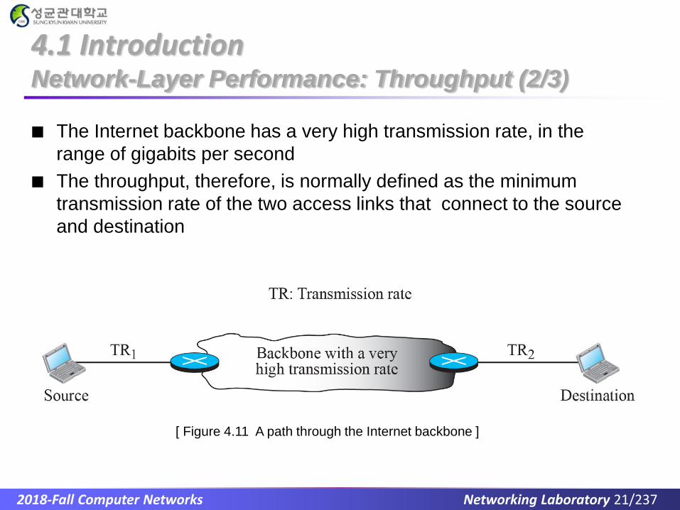
The Internet backbone has a very high transmission rate, in the
range of gigabits per second
The throughput, therefore, is normally defined as the minimum
transmission rate of the two access links that connect to the source
and destination
4.1 Introduction Network-Layer Performance: Throughput (2/3)
[ Figure 4.11 A path through the Internet backbone ]

2018-Fall Computer Networks Networking Laboratory 22/237
Besides, the link between two routers is not always dedicated to one
flow. A router may collect the flow from several sources or distribute
the flow between several sources. In this case the transmission rate
is actually shared between the flows
[ Fig 4.12 Effect of throughput is shared links ]
4.1 Introduction Network-Layer Performance: Throughput (3/3)

2018-Fall Computer Networks Networking Laboratory 23/237
When a router receives a packet while processing another packet, the
received packet needs to be stored in the input buffer. A router,
however, has an input buffer with a limited size
A time may come when the buffer is full and the next packet needs to
be dropped
The effect of packet loss on the Internet network layer is that the
packet needs to be resent, which in turn may create overflow and
cause more packet loss
4.1 Introduction Network-Layer Performance: Packet loss

2018-Fall Computer Networks Networking Laboratory 24/237
The study of congestion in this layer may only help us to better
understand cause of congestion at the transport layer and find possible
remedies to be used in network layer
There are two issues related: Packet delay and throughput
[ Fig 4.13 Packet delay and throughput as functions of load ]
4.1 Introduction Network-Layer Congestion

2018-Fall Computer Networks Networking Laboratory 25/237
Open-loop congestion control: prevents congestion before it
happens.
► Retransmission policy: retransmission is sometimes unavoidable.
Retransmission in general may increase congestion in the network.
However, a good retransmission policy can prevent congestion
► Window policy: the type of window at the sender which consists of Go-
Back-N window and Selective Repeat window also effect congestion.
Go-Back-N window: when the timer for a packet time out, several packets
may be resent, even some may have arrived safe
Selective Repeat window: tries to send the specific packets that have been
lost or corrupted
4.1 Introduction Network-Layer Congestion: Congestion control (1/4)

2018-Fall Computer Networks Networking Laboratory 26/237
Open-loop congestion control:
► Acknowledgement policy: imposed by the receiver also effect
congestion. If the receiver does not acknowledge every packet it
receives, it may slow down the sender and help prevent congestion
► Discard policy: operated by routers may prevent congestion and not
harm the integrity of the transmission
► Admission policy: is a quality-of-service mechanism (discussed in
chapter 8), can also prevent congestion in virtual-circuit networks
4.1 Introduction Network-Layer Congestion: Congestion control (2/4)

2018-Fall Computer Networks Networking Laboratory 27/237
Closed-loop congestion control: tries to alleviate congestion after it
happens
► Backpressure
► Choke packet
[ Fig 4.14 Backpressure method for alleviating congestion ]
[ Fig 4.15 Choke packet ]
4.1 Introduction Network-Layer Congestion: Congestion control (3/4)

2018-Fall Computer Networks Networking Laboratory 28/237
Closed-loop congestion control:
► Implicit Signaling: there is no communication between the congested
node or nodes and the source. The source guesses that there is
congestion somewhere in the network from other symptoms
► Explicit Signaling: Explicit signaling can occur in either the forward or the
backward direction which can be seen in an ATM network. It will be
discussed in Chapter 5
4.1 Introduction Network-Layer Congestion: Congestion control (4/4)

2018-Fall Computer Networks Networking Laboratory 29/237
Practice Problem (1/4)
Consider the following network path with 3 links and two store and
forward packet switches
► Note that each switch has 1.5 MB of memory for doing store and forward.
Assume that the processing delay at switches is 0 sec. The transmission
rate and the propagation delays of the links are as indicated in the picture

2018-Fall Computer Networks Networking Laboratory 30/237
Practice Problem (2/4)
What’s the maximum size of data this network path can carry at any
moment?

2018-Fall Computer Networks Networking Laboratory 31/237
Practice Problem (3/4) (cont.)
A MP3 file is roughly 4MB, how many MP3 files the path can carry at
any moment?

2018-Fall Computer Networks Networking Laboratory 32/237
Practice Problem (4/4)
Calculate the total time required to transfer a 1.5 MB file in the following
case, assuming RTT of 80 ms, and an initial handshaking before the file
is sent

2018-Fall Computer Networks Networking Laboratory 33/237
A router has four components: input ports, output ports, the routing
processor, and the switching fabric
[ Fig 4.16 Router components ]
4.1 Introduction Structure of A Router: Components (1/6)

2018-Fall Computer Networks Networking Laboratory 34/237
Input ports
Output ports
[ Fig 4.17 Input port ]
[ Fig 4.18 Output port ]
4.1 Introduction Structure of A Router: Components (2/6)

2018-Fall Computer Networks Networking Laboratory 35/237
4.1 Introduction Structure of A Router: Components (3/6)
Routing Processor
► Performing the function of the network layer
► Finding the address of the next hop and, at the same time, the
output port number from which packet is sent out
► This activity is sometimes referred to as table lookup because the
routing processor searches the forwarding table

2018-Fall Computer Networks Networking Laboratory 36/237
Switching Fabrics
[ Fig 4.20 Banyan switch ] [ Fig 4.19 Crossbar switch ]
4.1 Introduction Structure of A Router: Components (4/6)

2018-Fall Computer Networks Networking Laboratory 37/237
4.1 Introduction Structure of A Router: Components (5/6)
Switching Fabrics
► Banyan switch
[ Figure 4.21: Examples of routing in a banyan switch ]

2018-Fall Computer Networks Networking Laboratory 38/237
Batcher-Banyan switch: design a switch that comes before the banyan
switch and sorts incoming packets according to their destination
[ Fig 4.22 Batcher-Banyan switch ]
4.1 Introduction Structure of A Router: Components (6/6)

2018-Fall Computer Networks Networking Laboratory 39/237
4.2 Network-Layer Protocol
In this section, we show how the network layer is implemented in the
TCP/IP protocol suite
The protocols in the network layer have gone through several
versions
We concentrate on the current version (4), in the last section of this
chapter, we briefly discuss version 6, which is on the horizon

2018-Fall Computer Networks Networking Laboratory 40/237
4.2 Network-Layer Protocol
In this section, we show how the network layer is implemented in the
TCP/IP protocol suite
The network layer in version 4 can be thought of as one main protocol
and three auxiliary protocols:
► Internet Protocol ver. 4 (IPv4), main protocol, is responsible for packetizing,
forwarding and delivery of packet
► Internet Control Message Protocol ver. 4 (ICMPv4) helps IPv4 to handle
some errors in the network-layer delivery
► Internet Group Management Protocol (IGMP) helps IPv4 in multicasting
► Address Resolution Protocol (ARP) glues the network and data-link layer

2018-Fall Computer Networks Networking Laboratory 41/237
4.2 Network-Layer Protocol Network layer protocol in TCP/IP protocol suite
[ Fig 4.23 Position of IP and other network-layer protocols in TCP/IP protocol suite ]

2018-Fall Computer Networks Networking Laboratory 42/237
4.2 Network-Layer Protocol IP Datagram Format (1/11)
Packets used by the IP are called IP datagrams
[ Fig 4.24 IP datagram ]

2018-Fall Computer Networks Networking Laboratory 43/237
4.2 Network-Layer Protocol IP Datagram Format (2/11)
Version (VER)
► 4-bit field which defines the version of the IP protocol
► Currently the version is 4
► Version 6 may totally replace version 4 in the future
► If the machine is using some other version of IP, the datagram is discarded
Header length (HLEN)
► 4-bit field which defines the total length of the datagram header
in 4-byte words
► This field is needed because the head length is variable
Service type
► 8-bit field which was referred to as type of service (TOS)

2018-Fall Computer Networks Networking Laboratory 44/237
4.2 Network-Layer Protocol IP Datagram Format (3/11)
Total length
► 16-bit field which defines the total length of the IP datagram in bytes
► Length of data = total length – header length
► This field is necessary in case that the padding is added in the frame
Identification: 16-bit field which is used in fragmentation
L2 header
L2 Trailer
Data < 46 bytes Padding
Length: Minimum 46 bytes
[ Encapsulation of a small datagram in an Ethernet frame ]

2018-Fall Computer Networks Networking Laboratory 45/237
4.2 Network-Layer Protocol IP Datagram Format (4/11)
Flags
► 3-bit field which is used in fragmentation
Time to live
► A datagram has a limited lifetime in its travel through an internet
► This field is originally designed to hold a timestamp, which was
decremented by each visited router
► This field is mostly used to control the maximum number of hops visited by
the datagram. This value is approximately two times the maximum number
of routers between any two hosts
► If the value is zero, the router discards the datagram

2018-Fall Computer Networks Networking Laboratory 46/237
4.2 Network-Layer Protocol IP Datagram Format (5/11)
Protocol: 8-bit field which defines the higher level protocol that uses
the services of the IP layer
[ Figure 4.25: Multiplexing and demultiplexing using the value of the protocol field ]

2018-Fall Computer Networks Networking Laboratory 47/237
4.2 Network-Layer Protocol IP Datagram Format (6/11)
Checksum
► 16-bit field used for error check using checksum
Source address
► 32-bit field which defines the IP address of the source
Destination address
► 32-bit field which defines the IP address of the destination

2018-Fall Computer Networks Networking Laboratory 48/237
4.2 Network-Layer Protocol IP Datagram Format (7/11)
Maximum Transfer Unit: when a datagram is encapsulated in a
frame, the total size of the datagram must be less than MTU
[ Figure 4.26: Maximum transfer unit (MTU) ]

2018-Fall Computer Networks Networking Laboratory 49/237
4.2 Network-Layer Protocol IP Datagram Format (8/11)
Fields Related to Fragmentation:
► Fragmentation is to divide the datagram to make it possible to pass
through a network
► The source usually does not fragment the IP packet
► When a datagram is fragmented, each fragment has its own header with
most of the fields repeated, but some changed
► The reassembly of the datagram is done only by the destination host

2018-Fall Computer Networks Networking Laboratory 50/237
4.2 Network-Layer Protocol IP Datagram Format (9/11)
Fields Related to Fragmentation
► Identification (16-bit)
This field identifies a datagram originating from the source host
The combination of the identification and source IP address must uniquely define
a datagram as it leaves the source host
The identification number helps the destination in reassembling the datagram
► Flags (3-bit)
The first bit is reserved
The second bit is called the do not fragment bit
The third bit is called the more fragment bit
D M
D: Do not fragment
M: more fragment

2018-Fall Computer Networks Networking Laboratory 51/237
4.2 Network-Layer Protocol IP Datagram Format (10/11)
Fields Related to Fragmentation
► Fragmentation offset (13-bit)
This is offset of the data in the original datagram measured in units of 8 bytes
[ Fig 4.27 Fragmentation examples ]

2018-Fall Computer Networks Networking Laboratory 52/237
4.2 Network-Layer Protocol IP Datagram Format (11/11)
An example of fragmentation
[ Fig 4.28 Detailed fragmentation example ]

2018-Fall Computer Networks Networking Laboratory 53/237
Practice Problem
An IP message 12,000 bytes wide (including the 20-byte IP header) that
needs to be sent over a link with an MTU of 3,300 bytes.

2018-Fall Computer Networks Networking Laboratory 54/237
4.2 Network-Layer Protocol IP Datagram Format: Security of IPv4 (1/2)
In this section, we only give a brief idea about the security issues in IP
protocol and the solution. There are 3 issues:
► Packet Sniffing: a passive attack, in which the attacker does not change
the contents of data packet
► Packet Modification: the attacker intercepts the packet, changes its
contents, and sends the new packet to the receiver
► IP Spoofing: An attacker can masquerade as somebody else and create
an IP packet that carries the source address of another computer
► IPSec: used in conjunction with the IP protocol, creates a connection-
oriented service between two entities in which they can exchange IP
packets

2018-Fall Computer Networks Networking Laboratory 55/237
4.2 Network-Layer Protocol IP Datagram Format: Security of IPv4 (2/2)
► IPSec: used in conjunction with the IP protocol, creates a connection-
oriented service between two entities in which they can exchange IP
packets
Defining Algorithm and Keys: The two entities that want to create a secure
channel between themselves can agree on some available algorithms and keys
to be used for security purposes
Packet Encryption: The packets exchanged between two parties can be
encrypted for privacy using one of the encryption algorithms and a shared key
agreed upon in the first step
Data Integrity: Data integrity guarantees that the packet is not modified during
the transmission
Origin Authentication: IPSec can authenticate the origin of the packet to be
sure that the packet is not created by an imposter

2018-Fall Computer Networks Networking Laboratory 56/237
4.2 Network-Layer Protocol IPv4 address
An IP address is a 32-bit address
The IP addresses are unique
The address space of IPv4 is 232 or 4, 294, 967, 296
Notation
► Binary Notation : In binary notation, the IP address is displayed as 32
bits
► Dotted-Decimal Notation : Internet addresses are usually written in
decimal form with a decimal point separating the bytes
[ Fig 4.29 Three different notations in IPv4 addressing ]

2018-Fall Computer Networks Networking Laboratory 57/237
4.2 Network-Layer Protocol IPv4 address: Hierarchy in addressing
A 32-bit IPv4 address is hierarchical, but divided only into two parts
The first part of the address called the prefix, defines the network
The second part of the address called the suffix, defined the node
[ Fig 4.30 Hierarchy in addressing ]

2018-Fall Computer Networks Networking Laboratory 58/237
4.2 Network-Layer Protocol IPv4 address: Classful addressing
In classful addressing, the IP address space is divided into five classes:
A, B, C, D, E
[ Fig 4.31 Occupation of the address space in classful addressing ]

2018-Fall Computer Networks Networking Laboratory 59/237
4.2 Network-Layer Protocol IPv4 address: Address Depletion
The addresses being rapidly used up. So, no more addresses
available for organizations or individuals that needed to be connected
to the Internet
Class A with 16,777,216 IPs. Since there may be only a few
organizations that are this large, most of the addresses in this class
were wasted
Class B addresses were designed for midsize organization, but many
of the addresses also remained unused
Class C has only 256 IPs, it was so small that most companies were
not comfortable using a block in this address
Class E were almost never used, wasting the whole class

2018-Fall Computer Networks Networking Laboratory 60/237
4.2 Network-Layer Protocol IPv4 address: Subnetting and Supernetting
Subnetting and Supernetting are proposed to alleviate
address depletion
► In Subnetting, Class A or B is divided into several subnets. Each
subnet has a larger prefix length than the original network. In other
words, we divide a large block into smaller block
This idea did not work because most large organizations were not
happy about dividing the block and giving some of the unused
addresses to smaller organizations
► In Supernetting, we combine several class C blocks into a larger
block to be attractive to organizations that need more than 256 IPs
This idea did not work either because it makes the routing of packets more
difficult

2018-Fall Computer Networks Networking Laboratory 61/237
4.2 Network-Layer Protocol IPv4 address: Classless addressing (1/7)
In classless addressing, variable-length blocks are used that belong to
no classes. We can have a block of 1 address, 2 addresses, 4
addresses, 128 addresses, and so on
The prefix in an address defines the block (network); the suffix defines
the node (device). Therefore, we can have a block of 20, 21, 22,…, 232
addresses
► A small prefix means a larger network; a large prefix means a smaller
network
[ Figure 4.32: Variable-length blocks in classless addressing ]

2018-Fall Computer Networks Networking Laboratory 62/237
4.2 Network-Layer Protocol IPv4 address: Classless addressing (2/7)
Restrictions
► Number of Addresses in a Block
The number of addresses in a block must be a power of two
► First Address
The first address must be evenly divisible by the number of addresses
► Mask
In classless addressing, the address must be accompanied by the mask
The mask is given in classless inter-domain routing or CIDR notation with the
number of 1s
Format of classless addressing address is X.Y.Z.t/n, the n after the slash
defines the number of bits that are the same in every address in the block

2018-Fall Computer Networks Networking Laboratory 63/237
4.2 Network-Layer Protocol IPv4 address: Classless addressing (3/7)
Mask
► Prefix is another name for the common part of the address range, similar to
the netid in classful addressing
► Prefix length is the length of the prefix (n in the CIDR notation)
► Classful addressing is a special case of classless addressing
/n Mask /n Mask /n Mask /n Mask
/1 128.0.0.0 /9 255.128.0.0 /17 255.255.128.0 /25 255.255.255.128
/2 192.0.0.0 /10 255.192.0.0 /18 255.255.192.0 /26 255.255.255.192
/3 224.0.0.0 /11 255.224.0.0 /19 255.255.224.0 /27 255.255.255.224
/4 240.0.0.0 /12 255.240.0.0 /20 255.255.240.0 /28 255.255.255.240
/5 248.0.0.0 /13 255.248.0.0 /21 255.255.248.0 /29 255.255.255.248
/6 252.0.0.0 /14 255.252.0.0 /22 255.255.252.0 /30 255.255.255.252
/7 254.0.0.0 /15 255.254.0.0 /23 255.255.254.0 /31 255.255.255.254
/8 255.0.0.0 /16 255.255.0.0 /24 255.255.255.0 /32 255.255.255.255

2018-Fall Computer Networks Networking Laboratory 64/237
4.2 Network-Layer Protocol IPv4 address: Classless addressing (4/7)
Mask
► The suffix is the varying part, similar to the hostid
► The suffix length is the length of the suffix (32-n) in CIDR notation
[ Fig 4.34 Information extraction in classless addressing ]

2018-Fall Computer Networks Networking Laboratory 65/237
4.2 Network-Layer Protocol IPv4 address: Classless addressing (5/7)
Example 4.1: A classless address is given as 167.199.170.82/27. We
can find the above three pieces of information as follows
► The number of addresses in the network is 232− n= 25 = 32 addresses.
► The first address can be found by keeping the first 27 bits and changing the
rest of the bits to 0s
► The last address can be found by keeping the first 27 bits and changing the
rest of the bits to 1s

2018-Fall Computer Networks Networking Laboratory 66/237
4.2 Network-Layer Protocol IPv4 address: Classless addressing (6/7)
Example 4.2: We repeat Example 4.1 using the mask. The mask in
dotted-decimal notation is 255.255.255.224. The AND, OR, and NOT
operations can be applied to individual bytes using calculators and
applets at the book website

2018-Fall Computer Networks Networking Laboratory 67/237
4.2 Network-Layer Protocol IPv4 address: Classless addressing (7/7)
Example 4.3: In classless addressing, an address cannot per se define
the block the address belongs to. For example, the address 230.8.24.56
can belong to many blocks. Some of them are shown below with the
value of the prefix associated with that block

2018-Fall Computer Networks Networking Laboratory 68/237
4.2 Network-Layer Protocol IPv4 address: Network address (1/6)
The first address of the address block, network address, is particularly
important because it is used in routing a packet to its destination
network
First address = (prefix in decimal) * 232-n = (prefix in decimal) * N
[ Fig 4.35 Network address ]

2018-Fall Computer Networks Networking Laboratory 69/237
4.2 Network-Layer Protocol IPv4 address: Network address (2/6)
An ISP has requested a block of 1000 addresses. Since 1000 is not a
power of 2, 1024 addresses are granted
► The prefix length is calculated as n = 32 − log21024 = 22. An available
block, 18.14.12.0/22, is granted to the ISP

2018-Fall Computer Networks Networking Laboratory 70/237
4.2 Network-Layer Protocol IPv4 address: Network address (3/6)
An organization is granted a block of addresses with the beginning
address 14.24.74.0/24. The organization needs to have 3 subblocks
of addresses to use in its three subnets: one subblock of 10
addresses, one subblock of 60 addresses, and one subblock of 120
addresses. Design the subblocks
► There are 232– 24 = 256 addresses in this block
The first address is 14.24.74.0/24
The last address is 14.24.74.255/24
► To satisfy the third requirement, we assign addresses to subblocks,
starting with the largest and ending with the smallest one

2018-Fall Computer Networks Networking Laboratory 71/237
4.2 Network-Layer Protocol IPv4 address: Network address (4/6)
► The number of addresses in the largest subblock, which
requires 120 addresses, is not a power of 2
We allocate 128 addresses
The subnet mask for this subnet can be found as n1= 32 − log2 128 = 25
The first address in this block is 14.24.74.0/25; the last address is
14.24.74.127/25
► The number of addresses in the second largest subblock,
which requires 60 addresses, is not a power of 2 either
We allocate 64 addresses
The subnet mask for this subnet can be found as n2 = 32 − log2 64 = 26
The first address in this block is 14.24.74.128/26; the last address is
14.24.74.191/26

2018-Fall Computer Networks Networking Laboratory 72/237
4.2 Network-Layer Protocol IPv4 address: Network address (5/6)
► The number of addresses in the largest subblock, which requires 10
addresses, is not a power of 2
We allocate 16 addresses
The subnet mask for this subnet can be found as n1= 32 − log2 16 = 28.
The first address in this block is 14.24.74.192/28; the last address is
14.24.74.207/28
► If we add all addresses in the previous subblocks, the result is 208
addresses, which means 48 addresses are left in reserve.
The first address in this range is 14.24.74.208.
The last address is 14.24.74.255.
We don’t know about the prefix length yet. Figure 4.36 shows the
configuration of blocks. We have shown the first address in each block.

2018-Fall Computer Networks Networking Laboratory 73/237
4.2 Network-Layer Protocol IPv4 address: Network address (6/6)
[ Figure 4.36: Solution to Example 5 ]
14.24.74.192/28

2018-Fall Computer Networks Networking Laboratory 74/237
4.2 Network-Layer Protocol IPv4 address: Address aggregation
One of the advantages of the CIDR strategy is address aggregation.
When blocks of addresses are combined to create a larger block,
routing can be done based on prefix of the larger block
[ Fig 4.37 Example of address aggregation ]

2018-Fall Computer Networks Networking Laboratory 75/237
4.2 Network-Layer Protocol IPv4 address: Special addresses
This-host address: It is used whenever a host needs to send an IP
datagram but it does not know its own address to use as the source
address: 0.0.0.0/32
Limited-broadcast address: when router want to send data to all
devices: 255.255.255.255/32
Loopback address: one of the addresses is always as a destination
address: 127.0.0.0/8
Private addresses:
► 10.0.0.0/8
► 172.16.0.0/12
► 192.168.0.0/16
► 169.254.0.0/16 We will see the application of these addresses when we
discuss NAT later
Multicast addresses: is reserved for multicast addresses: 224.0.0.0/4

2018-Fall Computer Networks Networking Laboratory 76/237
Practice Problem
For the IP address 109.190.10.164/16,
► Find the First useable IP address
► Find the Broadcast address
► Find the Last useable IP address

2018-Fall Computer Networks Networking Laboratory 77/237
4.2 Network-Layer Protocol IPv4 address: DHCP (1/8)
Dynamic Host Configuration Protocol (DHCP)
► A large organization or an ISP can receive a block of addresses directly
from ICANN (Internet Corporation for Assigned Names and Numbers)
► A small organization can receive a block of addresses from an ISP
► Address assignment in an organization can be done automatically using the
Dynamic Host Configuration Protocol (DHCP)
► Permanent or temporary IP addresses are assigned to hosts

2018-Fall Computer Networks Networking Laboratory 78/237
4.2 Network-Layer Protocol IPv4 address: DHCP (2/8)
DHCP Message Format
[ Fig 4.38 DHCP message format ]
[ Fig 4.39 Option format ]

2018-Fall Computer Networks Networking Laboratory 79/237
4.2 Network-Layer Protocol IPv4 address: DHCP (3/8)
The joining host creates a DHCPDISCOVER message where only the
transaction-ID field is set to a random number
The DHCP server or servers responds with a DHCPOFFER message in
which the your-IP-address field defines the offered IP address for the
joining host and the server-IP-address includes the IP address of the
server
The joining host receives one or more offers and selects the best of
them. The joining host then sends a DHCPREQUEST message to the
server that has given the best offer
The selected server responds with an DHCPACK message

2018-Fall Computer Networks Networking Laboratory 80/237
4.2 Network-Layer Protocol IPv4 address: DHCP (4/8)
DHCP Operation
[ Fig 4.40 Operation of DHCP ]

2018-Fall Computer Networks Networking Laboratory 81/237
4.2 Network-Layer Protocol IPv4 address: DHCP (5/8)
Video Content
► How a computer gets its IP address
► An explanation of DHCP and how it works.
► Link: https://www.youtube.com/watch?v=RUZohsAxPxQ

2018-Fall Computer Networks Networking Laboratory 82/237
4.2 Network-Layer Protocol IPv4 address: DHCP (6/8)
DHCP Operation
https://www.youtube.com/watch?v=RUZohsAxPxQ
2018-Fall Computer Networks Networking Laboratory 83/237
4.2 Network-Layer Protocol IPv4 address: DHCP (7/8)
Two Well-known Ports
► DHCP uses two well-known ports: 68 and 67
Using FTP
► The server does not send all information that a client may need for joining
the network
► In DHCPACK message, the server defines the pathname of a file in which
the client can find the complete information
Error Control
► DHCP uses the service of UDP, which is not reliable
► To provide error control, DHCP uses two strategies:
Requires that UDP uses the checksum
Requires DHCP client uses timers and a retransmission policy if it
does not receive DHCP reply to a request

2018-Fall Computer Networks Networking Laboratory 84/237
4.2 Network-Layer Protocol IPv4 address: DHCP (8/8)
To provide dynamic address allocation, the DHCP client acts as state
machine that performs transitions from one state to another
[ Fig 4.41 FSM for the DHCP client ]

2018-Fall Computer Networks Networking Laboratory 85/237
4.2 Network-Layer Protocol IPv4 address: NAT (1/4)
Network Address Translation(NAT)
► This technology can provide the mapping between the private and universal
addresses and at the same time support virtual private networks
[ Figure 4.42: NAT ]

2018-Fall Computer Networks Networking Laboratory 86/237
4.2 Network-Layer Protocol IPv4 address: NAT (2/4)
[ Figure 4.43: Address translation ]

2018-Fall Computer Networks Networking Laboratory 87/237
4.2 Network-Layer Protocol IPv4 address: NAT (3/4)
[ Fig 4.44 Translation ]

2018-Fall Computer Networks Networking Laboratory 88/237
4.2 Network-Layer Protocol IPv4 address: NAT (4/4)
Using both IP addresses and port addresses
► To allow a many-to-many relationship between private-network hosts and
external server programs
► The translation table includes source and destination port addresses and
the transport layer protocol
[ Table 4.1 Five-column translation table ]

2018-Fall Computer Networks Networking Laboratory 89/237
4.2 Network-Layer Protocol Forwarding of IP Packets: Forwarding Techniques (1/4)
Next-Hop Method: the routing table holds only the address of the next
hop
Destination Next Hop
Host B R1
Destination Next Hop
Host B R2
Destination Next Hop
Host B -
Network Network Network R1 R2
Host A Host B
Destination Route
Host B R1, R2, Host B
Destination Route
Host B R2, Host
Destination Route
Host B Host B
Routing tables based on route
[ Routing tables based on next hop ]

2018-Fall Computer Networks Networking Laboratory 90/237
4.2 Network-Layer Protocol Forwarding of IP Packets: Forwarding Techniques (2/4)
Network-Specific Method: only one entry that defines the address of the
destination network itself
N1 N2
R1
S
A B C
D
Destination Next Hop
A B C D
R1 R1 R1 R1
Destination Next Hop
N2 R1
Routing table for host S based
on host-specific method
Routing table for host S based
on network-specific method

2018-Fall Computer Networks Networking Laboratory 91/237
4.2 Network-Layer Protocol Forwarding of IP Packets: Forwarding Techniques (3/4)
Host-Specific Method:
► The destination host address is given in the routing table
► Efficiency is sacrificed
N1
Destination Next Hop
Host B N2 N3 …
R1 R1 R3 …
N2 N3
R1 R3
R2
Host A
Routing table for host A
Host B

2018-Fall Computer Networks Networking Laboratory 92/237
4.2 Network-Layer Protocol Forwarding of IP Packets: Forwarding Techniques (4/4)
Default Method
N1
Destination Next Hop
N2 …
Default
R1 … R2
Host A
N2
R1
R2 Default
router
Routing table for host A
Rest of the Internet

2018-Fall Computer Networks Networking Laboratory 93/237
4.2 Network-Layer Protocol Forwarding of IP Packets: with Classless Addressing (1/7)
One column for the mask is needed to find the network address in a
routing table
At least four columns are needed in a routing table
Address Aggregation
► To reduce the number of entries in a routing table
► In this method, the blocks of addresses for several organizations are
aggregated into one larger block
Extract destination
address
Search table
Packet
Forwarding module
Next-hop address
and
interface number
To ARP
Mask (/n)
Network address
Next-hop
address
Interface number
… …
… …
… …
… …
[ Fig 4.45 Simplified forwarding
module in classless address ]

2018-Fall Computer Networks Networking Laboratory 94/237
4.2 Network-Layer Protocol Forwarding of IP Packets: with Classless Addressing (2/7)
Address Aggregation
140.24.7.0/26
140.24.7.64/26
140.24.7.128/26
140.24.7.192/26
Organization 1
Organization 2
Organization 3
Organization 4
m0 m4 m1
m2 m3
m0 m1
Mask Network address
Next-hop address
Interface
/26 /26 /26 /26 /0
140.24.7.0 140.24.7.64 140.24.7.128 140.24.7.192
0.0.0.0
- - - -
Default router
m0 m1 m2 m3 m4
Mask Network address
Next-hop address
Interface
/24 /0
140.24.7.0 0.0.0.0
- Default router
m0 m1
Routing table for R1
Routing table for R2
R1 R2
[ Fig 4.47 Address aggregation ]

2018-Fall Computer Networks Networking Laboratory 95/237
4.2 Network-Layer Protocol Forwarding of IP Packets: with Classless Addressing (3/7)
Longest Mask Matching
► In case that some organizations are not geographically close to the others
► The routing table is sorted from the longest mask to the shortest mask

2018-Fall Computer Networks Networking Laboratory 96/237
4.2 Network-Layer Protocol Forwarding of IP Packets: with Classless Addressing (4/7)
Longest Mask Matching
► Suppose a packet arrives at router R2 for organization 4 with destination address
140.24.7.200. The first mask at router R2 is applied, which gives the network address
140.24.7.192. The packet is routed correctly from interface m1 and reaches
organization 4
[ Fig 4.48 Longest mask matching ]

2018-Fall Computer Networks Networking Laboratory 97/237
4.2 Network-Layer Protocol Forwarding of IP Packets: with Classless Addressing (5/7)
Hierarchical Routing
► If the routing table has a sense of hierarchy like the Internet architecture,
the routing table can decrease in size
► If a block assigned to the local ISP starts with a.b.c.d/n, the ISP can create
blocks starting with e.f.g.h/m, m is greater than n
► The rest of the Internet does not have to know this division

2018-Fall Computer Networks Networking Laboratory 98/237
4.2 Network-Layer Protocol Forwarding of IP Packets: Forwarding with Classless
Addressing (6/7)
Hierarchical Routing
[ Fig 4.49 Hierarchical routing with ISPs ]

2018-Fall Computer Networks Networking Laboratory 99/237
4.2 Network-Layer Protocol Forwarding of IP Packets: with Classless Addressing (7/7)
Geographical Routing
► Extension of hierarchical routing
Routing Table Search Algorithms
► Searching in Classful Addressing
The routing table can be divided into three tables for efficiency
The default mask is applied to find the corresponding bucket
► Searching in Classless Addressing
The longest match can be used
Instead of list, other data structure such as a tree or a binary tree can be used

2018-Fall Computer Networks Networking Laboratory 100/237
4.2 Network-Layer Protocol Forwarding of IP Packets: based on label (1/3)
In a connection-oriented network, a switch forwards a packet based on
the label attached to the packet
[ Fig 4.51 Forwarding based on label ]

2018-Fall Computer Networks Networking Laboratory 101/237
4.2 Network-Layer Protocol Forwarding of IP Packets: based on label (2/3)
Multi-Protocol Label Switching (MPLS)
► When behaving like a router, MPLS can forward the packet based on the
destination address
► When behaving like a switch, it can forward a packet based on the label
► The MPLS header is actually a stack of sub headers that is used for
multilevel hierarchical switching
[ Fig 4.52 MPLS header added to an IP packet ]

2018-Fall Computer Networks Networking Laboratory 102/237
4.2 Network-Layer Protocol Forwarding of IP Packets: based on label (3/3)
Multi-Protocol Label Switching (MPLS)
► The MPLS header is actually a stack of subheaders that is used for
multilevel hierarchical switching
► Label: the label used to index the forwarding table in the router
► Exp: reserved
► S: if this is 1, the header is last on in the stack
► TTL: when it reaches zero, the packet is discarded
[ Fig 4.53 MPLS header made of a stack of labels ]

2018-Fall Computer Networks Networking Laboratory 103/237
4.2 Network-Layer Protocol ICMPv4
The Internet Control Message Protocol (ICMP) has been designed to
compensate the following two deficiencies:
► The IP protocol has no error-reporting or error-correcting mechanism
► The IP protocol has no built-in mechanism to notify the original host
► ICMP itself is a network layer protocol
► ICMP messages are first encapsulated inside IP datagrams before going to
the lower layer
Frame header
Frame data Trailer
IP header IP data
ICMP message

2018-Fall Computer Networks Networking Laboratory 104/237
4.2 Network-Layer Protocol ICMPv4: ICMP messages (1/6)
ICMP messages are first encapsulated inside IP datagrams before
going to the lower layer
Frame header
Frame data Trailer
IP header IP data
ICMP message

2018-Fall Computer Networks Networking Laboratory 105/237
4.2 Network-Layer Protocol ICMPv4: ICMP messages (2/6)
ICMP messages are divided into two broad categories
► The error-reporting messages report problems that a router or a
host(destination) may encounter when it processes an IP packet
► The query messages help a host or a network manager get specific
information from a router or another host
ICMP message
Error-reporting Query

2018-Fall Computer Networks Networking Laboratory 106/237
4.2 Network-Layer Protocol ICMPv4: ICMP messages (3/6)
ICMP messages
Category Type Message
Error-reporting messages
3 Destination unreachable
4 Source quench
11 Time exceeded
12 Parameter problem
5 Redirection
Query messages
8 or 0 Echo request or reply
13 or 14 Timestamp request or reply
17 or 18 Address mask request or reply
10 or 9 Router solicitation or advertisement

2018-Fall Computer Networks Networking Laboratory 107/237
4.2 Network-Layer Protocol ICMPv4: ICMP messages (4/6)
An ICMP message has an 8 bytes header and a variable size data
section
► In error-reporting messages, the data section carries information for finding
the original packet that had the error
► In query messages, the data section carries extra information based on the
type of the query
Type Code Checksum
Rest of header
Data section
8 bits 8 bits 8 bits 8 bits

2018-Fall Computer Networks Networking Laboratory 108/237
4.2 Network-Layer Protocol ICMPv4: ICMP messages (5/6)
Error-reporting messages
► ICMP always reports error messages to the original source
► No ICMP error messages will be generated in response to a datagram
carrying an ICMP error messages
► No ICMP error messages will be generated for a fragmented datagram that
is not the first fragment
► No ICMP error messages will be generated for a datagram having a
multicast address
► No ICMP error message will be generated for a datagram having a special
address such as 127.0.0.0 or 0.0.0.0
Error reports
Time exceeded
Source quench
Destination unreachable
Redirection Parameter problem

2018-Fall Computer Networks Networking Laboratory 109/237
4.2 Network-Layer Protocol ICMPv4: Destination Unreachable
When a router cannot route a datagram or a host cannot deliver a
datagram, the datagram is discarded
The router or the host sends a destination-unreachable message
back to the source host
Type : 3 Code: 0 to 15 Checksum
Unused (All 0s)
Part of the received IP datagram including IP header plus the first 8 bytes of the datagram data

2018-Fall Computer Networks Networking Laboratory 110/237
4.2 Network-Layer Protocol ICMPv4: Source Quench
The source-quench message in ICMP was designed to add a kind of
flow control to the IP
When a router or host discards a datagram due to congestion, it sends
a source-quench message to the sender of the datagram
► It informs the source that the datagram has been discarded
► It warns the source that there is congestion somewhere in the path and that
the source should slow down the sending process
One source-quench message is sent for each datagram that is
discarded due to congestion
Type : 4 Code : 0 Checksum
Unused (All 0s)
Part of the received IP datagram including IP header plus the first 8 bytes of the datagram data

2018-Fall Computer Networks Networking Laboratory 111/237
4.2 Network-Layer Protocol ICMPv4: Time Exceeded (1/3)
Whenever a router decrements a datagram with a time-to-live value to
zero, it discards the datagram and sends a time-exceeded message to
the original source (Code 0)
When the final destination does not receive all of the fragments in a set
time, it discards the received fragments and sends a time-exceeded
message to the original source (Code 1)
Type : 11 Code : 0 or 1 Checksum
Unused (All 0s)
Part of the received IP datagram including IP header plus the first 8 bytes of the datagram data

2018-Fall Computer Networks Networking Laboratory 112/237
4.2 Network-Layer Protocol ICMPv4: Time Exceeded (2/3)
The traceroute program can be used to trace the route of a packet from
the source to the destination
The traceroute program uses the ICMP messages and the TTL field in
the IP packet to find the route

2018-Fall Computer Networks Networking Laboratory 113/237
4.2 Network-Layer Protocol ICMPv4: Time Exceeded (3/3)
traceroute
[ Fig 4.55 Example of traceroute program ]

2018-Fall Computer Networks Networking Laboratory 114/237
4.2 Network-Layer Protocol ICMPv4: Parameter Problem
A parameter-problem message can be created by a router or the
destination host
► Code 0
There is an error ambiguity in one of the header fields
The value in the pointer field points to the byte with the problem
► Code 1
The required part of an option is missing
Type : 12 Code : 0 or 1 Checksum
Unused (All 0s)
Part of the received IP datagram including IP header plus the first 8 bytes of the datagram data
Pointer

2018-Fall Computer Networks Networking Laboratory 115/237
4.2 Network-Layer Protocol ICMPv4: Redirection (1/2)
A host usually starts with a small routing table that is gradually
augmented and updated
To update the routing table of the host, routers send a redirection
message to the host
LAN LAN
IP packet
IP packet IP packet
Redirection
message
R1 R2 B
A

2018-Fall Computer Networks Networking Laboratory 116/237
4.2 Network-Layer Protocol ICMPv4: Redirection (2/2)
Code 0
► Redirection for a network-specific route
Code 1
► Redirection for a host-specific route
Code 2
► Redirection for a network-specific route based on a specified type of service
Code 3
► Redirection for a host-specific route based on a specified type of service
Type : 5 Code : 0 to 3 Checksum
IP address of the target router
Part of the received IP datagram including IP header plus the first 8 bytes of the datagram data

2018-Fall Computer Networks Networking Laboratory 117/237
4.2 Network-Layer Protocol ICMPv4: Query Message
In this type of ICMP message, a node sends a message that is
answered in a specific format by the destination node
Query
Timestamp request and reply
Address-mask request and reply
Echo request and reply
Router solicitation and advertisement

2018-Fall Computer Networks Networking Laboratory 118/237
Practice Problem
How many DHCP packets are exchanged between a client and a server
before the client receives an IP address?

2018-Fall Computer Networks Networking Laboratory 119/237
4.2 Network-Layer Protocol ICMPv4: Echo Request and Reply (1/2)
An echo-request message can be sent by a host or router
An echo-reply message is sent by the host or router which receives an
echo-request message
Echo-request and echo-reply messages can be used by network
managers to check the operation of the IP protocol
Echo-request and echo-reply messages can test the reachability of a
host
Type : 8 or 0 Code : 0 Checksum
Optional data Sent by the request message; repeated by the reply
message
Sequence number Identifier

2018-Fall Computer Networks Networking Laboratory 120/237
4.2 Network-Layer Protocol ICMPv4: Echo Request and Reply (2/2)
The ping program is used to find if a host is alive and responding
► Ping approximate round trip times in milli-seconds
► The initial TTL packet value for an IP packet is 255 and then it is
decremented by 1 each time it encounters a router

2018-Fall Computer Networks Networking Laboratory 121/237
4.2 Network-Layer Protocol ICMPv4: Timestamp Request and Reply
Hosts and routers can use the timestamp-request and timestamp-reply
messages to determine the round-trip time needed for an IP datagram
to travel between them
Each timestamp field can hold a number representing time measured in
milliseconds from midnight in Universal Time
Type : 13 or 14 Code : 0 Checksum
Original timestamp
Sequence number Identifier
Receive timestamp
Transmit timestamp

2018-Fall Computer Networks Networking Laboratory 122/237
4.2 Network-Layer Protocol ICMPv4: Address-Mask Request and Reply
To obtain its mask, a host sends an address-mask-request message
to a router on the LAN
The router receiving the address-mask-request message responds with
an address-mask-reply message
The address-mask field is filled with zeros in the request message
Type : 17 or 18 Code : 0 Checksum
Address mask
Sequence number Identifier

2018-Fall Computer Networks Networking Laboratory 123/237
4.3 Unicast routing
In an internet, the goal of the network layer is to deliver a datagram
from its source to its destination or destinations.
If a datagram is destined for only one destination (one-to-one delivery),
we have unicast routing.
In this section and the next, we discuss only unicast routing; multicast
and broadcast routing will be discussed later in the chapter.

2018-Fall Computer Networks Networking Laboratory 124/237
4.3 Unicast routing General Idea: An Internet as a Graph
To find the best route, an internet can be modeled as a graph
We can think of each router as a node and each network between a
pair of routers as an edge
[ Fig 4.56 An internet and its graphical representation ]

2018-Fall Computer Networks Networking Laboratory 125/237
4.3 Unicast routing General Idea: Least-cost routing
When an internet is modeled as a weighted graph, one of the ways to
interpret the best route from the source router to the destination router
is to find the least cost between the two
If there are N routers in an internet, there are (N-1) least-cost paths
from each router to any other router
We need N*(N-1) least-cost paths for the whole internet

2018-Fall Computer Networks Networking Laboratory 126/237
4.3 Unicast routing General Idea: Least-cost-trees
A least-cost tree is a tree with the source router as the root that spans
the whole graph (visits all other nodes)
[ Fig 4.57 Least-cost trees for nodes in the internet ]

2018-Fall Computer Networks Networking Laboratory 127/237
4.3 Unicast routing Routing Algorithm: Distance vector routing(1/9)
In distance vector routing, the least cost route between any two nodes
is the route with minimum distance
[ Fig 4.58 The distance vector corresponding to a tree ]

2018-Fall Computer Networks Networking Laboratory 128/237
4.3 Unicast routing Routing Algorithm: Distance vector routing(2/9)
Bellman-Ford equation is used to find the least cost (shortest
distance) between a source node x, and a destination node y, through
some intermediary nodes (a, b, c,…)
[ Fig 4.59 Graphical idea behind Bellman-Ford equation ]

2018-Fall Computer Networks Networking Laboratory 129/237
4.3 Unicast routing Routing Algorithm: Distance vector routing(3/9)
Initialization: each node can know only the distance between itself and
its immediate neighbors
[ Fig 4.60 The first distance vector for an internet ]

2018-Fall Computer Networks Networking Laboratory 130/237
4.3 Unicast routing Routing Algorithm: Distance vector routing(4/9)
Sharing:
► A node is not aware of a neighbor’s table
► The best solution for each node is to send its entire table to the neighbor
and let the neighbor decide what part to use and what part to discard
► In distance vector routing, each node shares its routing table with its
immediate neighbors periodically and when there is a change

2018-Fall Computer Networks Networking Laboratory 131/237
4.3 Unicast routing Routing Algorithm: Distance vector routing(5/9)
Updating:
[ Fig 4.61 Updating distance vectors ]

2018-Fall Computer Networks Networking Laboratory 132/237
4.3 Unicast routing Routing Algorithm: Distance vector routing(6/9)
[ Table 4.4 Distance vector routing algorithm for a node ]

2018-Fall Computer Networks Networking Laboratory 133/237
4.3 Unicast routing Routing Algorithm: Distance vector routing(7/9)
Two-Node Loop Instability: A problem with distance vector routing is
instability
X A B
X 2 - X 6 A
2 4 Before failure
After failure
After A receives
update from B
Finally
X
X ∞ X 6 A
2 4 B A
X
X 10 B X 6 A
2 4 B A
X
X ∞ X ∞
2 4 B A
[ Fig 4.62 Two-node instability ]

2018-Fall Computer Networks Networking Laboratory 134/237
4.3 Unicast routing Routing Algorithm: Distance vector routing(8/9)
Solutions of two-node loop instability:
► Defining Infinity
Most implementations of the distance vector protocol define the distance
between each node to be 1 and define 16 as infinity
► Split Horizon
In this strategy, instead of flooding the table through each interface, each node
sends only part of its table through each interface
• Node B eliminates the last line of its forwarding table before it sends to A
► Poison Reverse
Node B can still advertise the value for X, but if the source information is A, it can
replace the distance with infinity as a warning: “Do not use this value; what I
know about this come from you”
2018-Fall Computer Networks Networking Laboratory 135/237
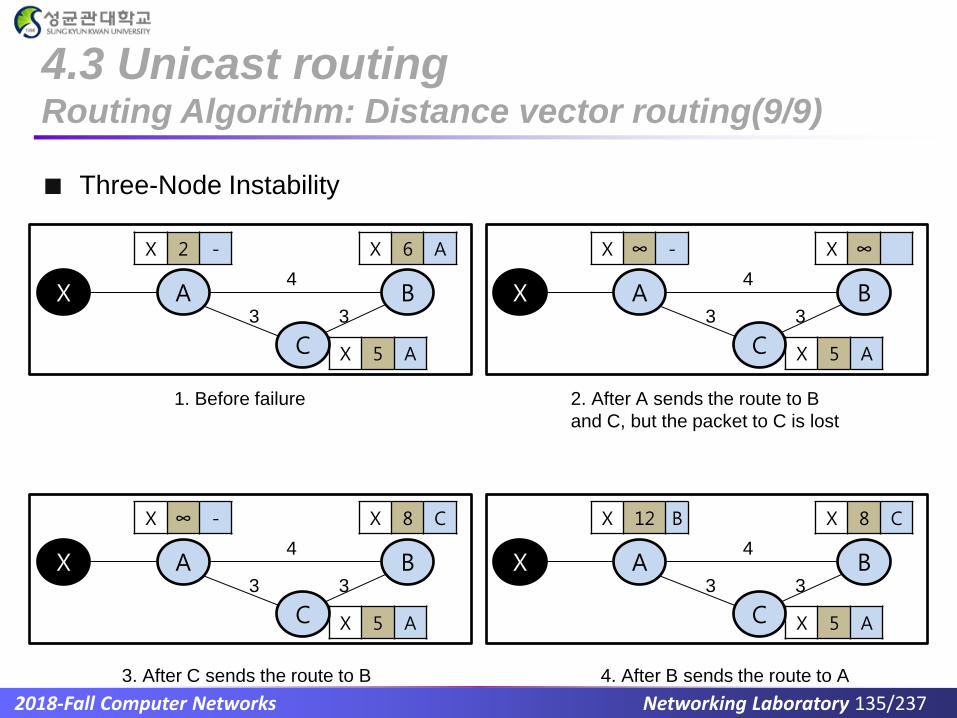
4.3 Unicast routing Routing Algorithm: Distance vector routing(9/9)
X A B
C
X 2 - X 6 A
X 5 A
X A B
C
X ∞ - X 8 C
X 5 A
X A B
C
X 12 B X 8 C
X 5 A
X A B
C
X ∞ - X ∞
X 5 A
4
3 3
4
3 3
4
3 3
4
3 3
1. Before failure 2. After A sends the route to B
and C, but the packet to C is lost
3. After C sends the route to B 4. After B sends the route to A
Three-Node Instability

2018-Fall Computer Networks Networking Laboratory 136/237
4.3 Unicast Routing Routing Algorithms: Link-State Routing (1/7)
Link-state (LS) routing is a routing algorithm for creating least-cost trees
and forwarding tables
Link-state database (LSDB)
► To create a least cost tree with this method, each node needs to have a
complete map of the network, which means it needs to know the state of
each link
► The collection of states for all links is called the link-state database.
[Fig 4.63 Example of a link-state database]

2018-Fall Computer Networks Networking Laboratory 137/237
4.3 Unicast Routing Routing Algorithms: Link-State Routing (2/7)
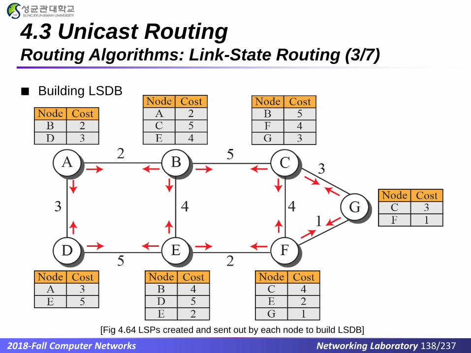
Building LSDB
► This can be done by a process called flooding.
1. Each node can send some greeting messages to all its immediate neighbors
(those nodes to which it is connected directly) to collect two pieces of
information for each neighboring node: the identity of the node and the cost of
the link.
2. The combination of these two pieces of information is called the LS packet
(LSP). LSP also includes a sequence number, which increases when a new
version of the LSP is created.
3. Each node creates the LSP and sends out of each interface.
• When a node receives an LSP, it compares the LSP with the copy it may already
have by checking the sequence number.
• Then, it discards the old LSP and keeps the new one and then sends a copy of it
out of each interface except the one from which the packet arrived.
4. After receiving all new LSPs, each node creates the comprehensive LSDB as
shown in Figure 4.64
2018-Fall Computer Networks Networking Laboratory 138/237
4.3 Unicast Routing Routing Algorithms: Link-State Routing (3/7)
Building LSDB
[Fig 4.64 LSPs created and sent out by each node to build LSDB]

2018-Fall Computer Networks Networking Laboratory 139/237
4.3 Unicast Routing Routing Algorithms: Link-State Routing (4/7)
Formation of Least-Cost Trees
► After receiving all LSPs, each node will have a copy of the whole topology
► A shortest path tree is needed
► The Dijkstra algorithm creates a shortest path tree from a graph

2018-Fall Computer Networks Networking Laboratory 140/237
4.3 Unicast Routing Routing Algorithms: Link-state routing (5/7)
Dijkstra’s algorithm Start
Set root to local node and
move it to permanent list
Tentative list
is empty?
Among nodes in tentative list, move the one
with the shortest path to permanent list
Add each unprocessed neighbor of last moved
node to tentative list if not already there.
If neighbor is in the tentative list with larger
cumulative cost, replace it with new one
Stop
No
Yes

2018-Fall Computer Networks Networking Laboratory 141/237
4.3 Unicast Routing Routing Algorithms: Link-State Routing (6/7)
► Dijkstra’s algorithm
[Fig 4.65 Least-cost tree]

2018-Fall Computer Networks Networking Laboratory 142/237
4.3 Unicast Routing Routing Algorithms: Link-State Routing (7/7)
► Dijkstra’s algorithm
[Table 4.5 Dijkstra’s algorithm]

2018-Fall Computer Networks Networking Laboratory 143/237
4.3 Unicast Routing Routing Algorithms: Path-Vector Routing (1/5)
Path Vector Routing
► Path vector routing is not based on least-cost routing
► Path vector routing is mostly designed to route a packet
between ISPs
Spanning trees
► The path from a source to all destinations is also determined
by the best spanning tree
► If there is more than one route to a destination, the source can choose the
route that meets its policy best
► A source may apply several policies at the same time. One of the common
policies uses the minimum number of nodes to be visited.

2018-Fall Computer Networks Networking Laboratory 144/237
4.3 Unicast Routing Routing Algorithms: Path-Vector Routing (2/5)
Spanning trees:
► Each source has created its own spanning tree that meets its policy
► The policy is to use the minimum number of nodes to reach a destination
[Fig 4.66 Spanning trees in path-vector routing]

2018-Fall Computer Networks Networking Laboratory 145/237
4.3 Unicast Routing Routing Algorithms: Path-Vector Routing (3/5)
Creation of spanning trees
► When a node is booted, it creates a path vector based on the information it
can obtain about its immediate neighbor
► A node sends greeting messages to its immediate neighbors to collect
these pieces of information
► Each node, after the creation of the initial path vector, sends it to all its
immediate neighbors.
► Each node, when it receives a path vector from a neighbor, updates its path
vector the equation:
Path(x, y) = best {path(x, y), [(x+path(v,y)]} for all v’s in the internet

2018-Fall Computer Networks Networking Laboratory 146/237
4.3 Unicast Routing Routing Algorithms: Path-Vector Routing (4/5)
Creation of spanning trees
[ Fig 4.67 path vectors made at booting time ]
[ Fig 4.68 Updating path vectors ]

2018-Fall Computer Networks Networking Laboratory 147/237
4.3 Unicast Routing Routing Algorithms: Path-Vector Routing (5/5)
Path-vector algorithm
[ Table 4.6 Path-vector algorithm for a node ]

2018-Fall Computer Networks Networking Laboratory 148/237
Practice Problem
Dijkstra shortest path algorithm example
A
D E
B C
D
1

2018-Fall Computer Networks Networking Laboratory 149/237
Practice Problem
What is the significance of name “Distance vector routing”

2018-Fall Computer Networks Networking Laboratory 150/237
4.3 Unicast Routing Unicast Routing Protocols: Introduction
Introduction
► Three common protocols used in the Internet are introduced
Routing Information Protocol (RIP): based on the distance-vector
algorithm
Open Shortest Path First (OSPF): based on the link-state algorithm
Border Gateway Protocol (BGP): based on the path-vector algorithm

2018-Fall Computer Networks Networking Laboratory 151/237
4.3 Unicast Routing Unicast Routing Protocols: Internet structure(1/2)
Internet structure
► Backbones: provide global connectivity
► Provider network: at a lower level, use the backbones for global connectivity
► Customer networks: use the services provided by the provider networks
► Any of these three entities can be called an Internet Service Provider or ISP,
but at different level
[ Fig 4.69 Internet structure ]

2018-Fall Computer Networks Networking Laboratory 152/237
4.3 Unicast Routing Unicast Routing Protocols: Internet structure(2/2)
Hierarchical Routing
► Hierarchical routing means considering each ISP as an
autonomous system (AS).
► Routing inside an AS is referred to as intradomain routing
► Global routing to glue all ASs together is referred to as
interdomain routing
Autonomous
system
Autonomous
system
Autonomous
system
Autonomous
system

2018-Fall Computer Networks Networking Laboratory 153/237
4.3 Unicast Routing Unicast Routing Protocols: RIP (1/10)
RIP
► The Routing Information Protocol (RIP) is an intradomain routing
protocol used inside an autonomous system
Hop Count
► RIP basically implements distance vector routing algorithm with some
considerations
The cost is defined as the number of hops, which means the
number of networks (subnets) a packet needs to travel through
from the source router to the final destination host
In RIP, the maximumcost of a path can be 15, which means
16 is considered as infinity (no connection)

2018-Fall Computer Networks Networking Laboratory 154/237
4.3 Unicast Routing Unicast Routing Protocols: RIP (2/10)
Forwarding Tables
3 hops (N2, N3, N4)
2 hops (N3, N4)
1 hop (N4)
[Fig 4.70 Hop counts in RIP]
[Fig 4.71 Forwarding tables]

2018-Fall Computer Networks Networking Laboratory 155/237
4.3 Unicast Routing Unicast Routing Protocols: RIP (3/10)
RIP Implementation
► RIP runs at the application layer, but creates forwarding tables for
IP at the network layer
► RIP uses UDP port 520 for route updates
► RIP has two versions RIP-1 and RIP-2. We discuss only RIP-2.

2018-Fall Computer Networks Networking Laboratory 156/237
4.3 Unicast Routing Unicast Routing Protocols: RIP (4/10)
RIP messages
► RIP has two types of messages: request and response
Command Version Reserved
Tag Family
Network address
Subnet mask
Next-hop address
Distance
Repeate
d
[Fig 4.72 RIP message format]

2018-Fall Computer Networks Networking Laboratory 157/237
4.3 Unicast Routing Unicast Routing Protocols: RIP (5/10)
RIP messages
► Request
A request message is sent by a router that has just come up or by a router that
has some time-out entries
► Response (or update)
A response can be either solicited or unsolicited
A solicited response is sent only in answer to a request
An unsolicited response is sent periodically, every 30s or when
there is a change in the routing table

2018-Fall Computer Networks Networking Laboratory 158/237
4.3 Unicast Routing Unicast Routing Protocols: RIP (6/10)
RIP algorithm
► RIP implements the same algorithm as the distance-vector routing
algorithm, but has some changes
A router needs to send the whole contents of its forwarding table in a response
message
The receiver adds one hop to each cost and changes the next router field to the
address of the sending router. Each route in the modified forwarding table is
called the received route and each route in the old forwarding table is called the
old route. The received router selects the old routes as the new ones except in
the following three cases:

2018-Fall Computer Networks Networking Laboratory 159/237
4.3 Unicast Routing Unicast Routing Protocols: RIP (7/10)
1. If the received route does not exist in the old forwarding table, it should be
added to the route.
2. If the cost of the received route is lower than the cost of the old one, the
received route should be selected as the new one.
3. If the cost of the received route is higher than the cost of the old
one, but the value of the next router is the same in both routes, the received
route should be selected as the new one.
• This is the case where the route was actually advertised by the same router in the
past, but now the situation has been changed.
• For example, suppose a neighbor has previously advertised a route to a destination
with cost 3, but now there is no path between this neighbor and that destination. The
neighbor advertises this destination with cost value infinity (16 in RIP)

2018-Fall Computer Networks Networking Laboratory 160/237
4.3 Unicast Routing Unicast Routing Protocols: RIP (8/10)
RIP algorithm
[ Fig 4.73 Example of an autonomous system using RIP ]

2018-Fall Computer Networks Networking Laboratory 161/237
4.3 Unicast Routing Unicast Routing Protocols: RIP (9/10)
Timer in RIP
► Periodic Timer
It controls the advertising of regular update messages
The working model uses a random number between 25 and 35s
It counts down; when zero is reached, the update message is sent
Timers
Expiration 180 s
Periodic 25~35 s
Garbage collection 120 s

2018-Fall Computer Networks Networking Laboratory 162/237
4.3 Unicast Routing Unicast Routing Protocols: RIP (10/10)
Timer in RIP (cont’d)
► Expiration Timer
It governs the validity of a route
If there is a problem on an internet and no update is received within the allotted
180s, the route is considered expired and the hop count of the route is set to 16
► Garbage Collection Timer
When the information about a route becomes invalid, the router does not
immediately purge that route from its table
It continues to advertise the route with a metric value of 16
At the same time, a timer called the garbage collection timer is set to 120s
When the count reaches zero, the route is purged

2018-Fall Computer Networks Networking Laboratory 163/237
4.3 Unicast Routing Unicast Routing Protocols: OSPF(1/15)
OSPF (Open Shortest Path First)
► OSPF is an intradomain routing protocol like RIP
► It is based on the link-state routing protocol
Metric
► Each link can be assigned a weight based on the throughput, RTT (round
trip time), reliability, hop count, and so on.
Total cost: 12
Total cost: 7
Total cost: 4
[ Fig 4.74 Metric in OSPF ]
2018-Fall Computer Networks Networking Laboratory 164/237
4.3 Unicast Routing Unicast Routing Protocols: OSPF(2/15)
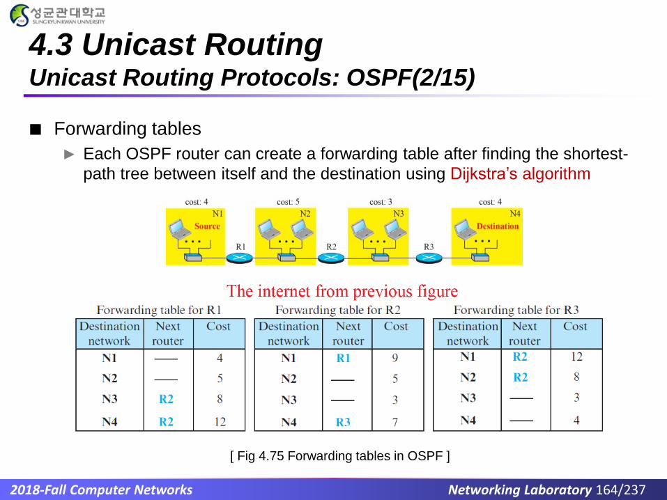
Forwarding tables
► Each OSPF router can create a forwarding table after finding the shortest-
path tree between itself and the destination using Dijkstra’s algorithm
[ Fig 4.75 Forwarding tables in OSPF ]

2018-Fall Computer Networks Networking Laboratory 165/237
4.3 Unicast Routing Unicast Routing Protocols: OSPF(3/15)
Areas
► OSPF divides an autonomous system into areas
► An area is a collection of networks, hosts, and routers all contained within
an autonomous system
► Area border routers summarize the information about the area and send it
to other areas
► All of the areas inside an autonomous system must be connected to a
special area called backbone
► If the connectivity between a backbone and an area is broken, a virtual link
between routers must be created

2018-Fall Computer Networks Networking Laboratory 166/237
4.3 Unicast Routing Unicast Routing Protocols: OSPF(4/15)
Areas
[ Fig 4.76 Areas in an autonomous system ]

2018-Fall Computer Networks Networking Laboratory 167/237
4.3 Unicast Routing Unicast Routing Protocols: OSPF(5/15)
Link-state advertisement
► Router link
A router link advertises the existence of a router as a node
A point-to-point link connects two routers without any other host or router in
between
A transient link is a network with several routers attached to it
A stub link is a network that is connected to only one router
[ Fig 4.77 Router link]

2018-Fall Computer Networks Networking Laboratory 168/237
4.3 Unicast Routing Unicast Routing Protocols: OSPF(6/15)
Link-state advertisement
► Network link
A network link advertises the network as a node
Since a network cannot do announcements itself, one of the routers is assigned
as the designated router and does the advertising
[ Fig 4.78 Network link]

2018-Fall Computer Networks Networking Laboratory 169/237
4.3 Unicast Routing Unicast Routing Protocols: OSPF(7/15)
Link-state advertisement
► Summary link to network
This is done by an area border router
It advertises the summary of links collected by the backbone to an area or the
summary of links collected by the area to the backbone
► Summary link to AS
This is done by an AS router
It advertises the summary links from other AS to the backbone area
► External link
This is done by an AS router to announce the existence of a single network
outside the AS

2018-Fall Computer Networks Networking Laboratory 170/237
4.3 Unicast Routing Unicast Routing Protocols: OSPF(8/15)
Link-state advertisement
[ Fig 4.79 Five different LSPs ]

2018-Fall Computer Networks Networking Laboratory 171/237
4.3 Unicast Routing Unicast Routing Protocols: OSPF(9/15)
OSPF Implementation
► OSPF is implemented as a program in the network layer that uses
the service of the IP for propagation.
► An IP datagram that carries a message from OSPF sets the value of the
protocol field to 89.
► There are two versions: version 1 and version 2. Most
implementations use version 2.

2018-Fall Computer Networks Networking Laboratory 172/237
4.3 Unicast Routing Unicast Routing Protocols: OSPF(10/15)
OSPF Messages
► Two message headers used in OSPF:
OSPF common header: is used in all messages.
The link-state general header: is used in some messages.
► Five message types used in OSPF:
Hello message: Used by a router to introduce itself to the neighbors and
announces all neighbors that it already knows
Database description message: Sent in response to the hello message to allow a
newly joined router to acquire the full LSDB
Link-state request message: Sent by a router that needs information about a
specific link state
Link-state update message: Used for building the LSDB
Link-state acknowledgment: Used to create reliability in OSPF

2018-Fall Computer Networks Networking Laboratory 173/237
4.3 Unicast Routing Unicast Routing Protocols: OSPF(11/15)
OSPF Messages
► Hello message
Used by a router to introduce itself to the neighbors and announces all neighbors
that it already knows
► Database description message
Sent in response to the hello message to allow a newly joined router to acquire
the full LSDB
► Link-state request message
Sent by a router that needs information about a specific link state

2018-Fall Computer Networks Networking Laboratory 174/237
4.3 Unicast Routing Unicast Routing Protocols: OSPF(12/15)
OSPF Messages
► Link-state update message
Used for building the LSDB
► Link-state acknowledgment
Used to create reliability in OSPF

2018-Fall Computer Networks Networking Laboratory 175/237
4.3 Unicast Routing Unicast Routing Protocols: OSPF(13/15)
OSPF Messages
[ Fig 4.80 OSPF message formats ]

2018-Fall Computer Networks Networking Laboratory 176/237
4.3 Unicast Routing Unicast Routing Protocols: OSPF(14/15)
OSPF Messages
[ Fig 4.81 OSPF message formats ]

2018-Fall Computer Networks Networking Laboratory 177/237
4.3 Unicast Routing Unicast Routing Protocols: OSPF(15/15)
OSPF Algorithm
► OSPF implements the link-state routing algorithm with some considerations:
After each router has created the shortest-path tree, the algorithm
needs to use it to create the corresponding routing algorithm
The algorithm needs to be augmented to handle sending and
receiving all five types of messages
2018-Fall Computer Networks Networking Laboratory 178/237
4.3 Unicast Routing Unicast Routing Protocols: Practice Problem
What is the difference between OSPF and RIP?

2018-Fall Computer Networks Networking Laboratory 179/237
4.3 Unicast Routing Unicast Routing Protocols: BGP4 (1/13)
BGP4: Border Gateway Protocol Version 4
► is the only interdomain routing protocol used in the Internet today
► BGP4 is based on the path-vector algorithm
► To enable each router to route a packet to any network in the internet,
external BGP4 (eBGP) is installed on each border router
► internal BGP (iBGP) is installed on all routers
[ Fig 4.82 A sample internet with four ASs ]

2018-Fall Computer Networks Networking Laboratory 180/237
4.3 Unicast Routing Unicast Routing Protocols: BGP4 (2/13)
Operation of external BGP
► Two routers, which eBGP is installed on, try to create a TCP connection
using the well-known port 179 as eBGP session.
The circled number defines the sending router in each case. For example,
message number 1 is sent by router R1 and tells router R5 that N1, N2, N3,and
N4 can be reached through router R1.
[ Fig 4.83 eBGP operation ]

2018-Fall Computer Networks Networking Laboratory 181/237
4.3 Unicast Routing Unicast Routing Protocols: BGP4 (3/13)
Operation of internal BGP
► It also uses the service of TCP on the well-known port 179, but it creates a
session between any possible pair of routers inside an autonomous system
► An AS router combines the reachability information about another AS with
the reachability information it already knows about the AS it belongs to
► Then the AS router sends a new update message to another AS
► In this way, all the network devices can transmit data to another in another
AS

2018-Fall Computer Networks Networking Laboratory 182/237
4.3 Unicast Routing Unicast Routing Protocols: BGP4 (4/13)
► The first message (numbered1) is sent by R1 announcing that networks N8 and N9
are reachable through the path AS1-AS2 to R2, R3, and R4. Routers R2, R4, and
R6 do the same thing, like R1, but send different messages to different destinations.
► When R1 receives the update message from R2, it combines the reachability
information about AS3 with the reachability information it already knows about AS1
and sends a new update message to R5. The process continues when R1 receives
the update message from R4.
[ Fig 4.84 Combination of eBGP and iBGP sessions in our Internet ]

2018-Fall Computer Networks Networking Laboratory 183/237
4.3 Unicast Routing Unicast Routing Protocols: BGP4 (5/13)
Operation of internal BGP
[ Fig 4.85 Finalized BGP path tables]
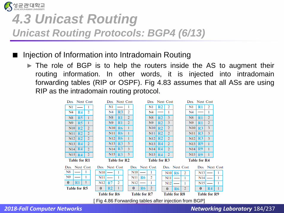
2018-Fall Computer Networks Networking Laboratory 184/237
4.3 Unicast Routing Unicast Routing Protocols: BGP4 (6/13)
Injection of Information into Intradomain Routing
► The role of BGP is to help the routers inside the AS to augment their
routing information. In other words, it is injected into intradomain
forwarding tables (RIP or OSPF). Fig 4.83 assumes that all ASs are using
RIP as the intradomain routing protocol.
[ Fig 4.86 Forwarding tables after injection from BGP]

2018-Fall Computer Networks Networking Laboratory 185/237
4.3 Unicast Routing Unicast Routing Protocols: BGP4 (7/13)
Path attributes
► Interdomain routing needs more information about how to reach the final
destination compared to intradomain routing
► These pieces(information) are called path attributes
[ Fig 4.87 Format of path attribute ]

2018-Fall Computer Networks Networking Laboratory 186/237
4.3 Unicast Routing Unicast Routing Protocols: BGP4 (8/13)
Path attributes
► ORIGIN (type 1)
A well-known mandatory attribute
Defines the source of the routing information
(1: RIP or OSPF, 2:BGP, 3: unknown source)
► AS-PATH (type 2)
A well-known mandatory attribute
Defines the list of autonomous systems through which the destination can be
reached
► NEXT-HOP
A well-known mandatory attribute
Defines the next router to which the data packet should be forwarded

2018-Fall Computer Networks Networking Laboratory 187/237
4.3 Unicast Routing Unicast Routing Protocols: BGP4 (9/13)
Path attributes
► MULTI-EXIT-DISC (type 4)
An optional non-transitive attribute
Discriminates among multiple exit paths to a destination
► LOCAL-PREF (type 5)
A well-known discretionary attribute
It is normally set by the administrator, based on the organization policy
The routes the administrator prefers are given a higher local preference

2018-Fall Computer Networks Networking Laboratory 188/237
4.3 Unicast Routing Unicast Routing Protocols: BGP4 (10/13)
Path attributes
► ATOMIC-AGGREGATE (type 6)
A well-known discretionary attribute
Defines the destination prefix; only single destination network
► AGGREGATOR (type7)
Optional transitive attribute
Emphasizes that the destination prefix is an aggregate

2018-Fall Computer Networks Networking Laboratory 189/237
4.3 Unicast Routing Unicast Routing Protocols: BGP4 (11/13)
Route Selection
► In the case where multiple routes are received to a destination, BGP needs
to select one among them.
[ Fig 4.88 Flow diagram for route selection]

2018-Fall Computer Networks Networking Laboratory 190/237
4.3 Unicast Routing Unicast Routing Protocols: BGP4 (12/13)
Messages
► Open message
To create a neighborhood relationship, a router running BGP opens a
TCP connection with a neighbor and sends an open message
► Update message
It is used by a router to withdraw destinations that have been advertised
previously, to announce a route to a new destination
► Keepalive message
BGP peers exchange keepalive messages regularly to tell each other they are
alive
► Notification
is sent when an error condition is detected or a router wants to close session

2018-Fall Computer Networks Networking Laboratory 191/237
4.3 Unicast Routing Unicast Routing Protocols: BGP4 (13/13)
Messages
[ Fig 4.89 BGP Messages]

2018-Fall Computer Networks Networking Laboratory 192/237
4.4 Multicasting Routing Introduction: Unicasting
Unicasting
► There is one source and one destination network
[ Fig 4.90 Unicasting ]

2018-Fall Computer Networks Networking Laboratory 193/237
4.4 Multicasting Routing Introduction: Multicasting (1/2)
Multicasting
► There is one source and a group of destinations
[ Fig 4.91 Multicasting ]

2018-Fall Computer Networks Networking Laboratory 194/237
4.4 Multicasting Routing Introduction: Multicasting (2/2)
Multicasting versus multiple unicasting
► Multicasting starts with a single packet from the source that is duplicated by
the routers
► In multiple unicasting, several packets start from the source
[ Fig 4.92 Multicasting versus multiple unicasting ]

2018-Fall Computer Networks Networking Laboratory 195/237
4.4 Multicasting Routing Introduction: Multicast Applications
Multicast applications
► Access to distributed databases
Most of the large databases today are distributed. A user’s request is multicast to
all the database locations, and the location that has the information responds
► Information dissemination
For example, a software update can be sent to all purchasers of a particular
software package. News can be easily disseminated through multicasting
► Teleconferencing
The individuals attending a teleconference all need to receive the same
information at the same time.
► Distance learning
Lessons taught by one professor can be received by a specific group of
students.

2018-Fall Computer Networks Networking Laboratory 196/237
4.4 Multicasting Routing Introduction: Broadcasting
Broadcasting
► One-to-all communication
Broadcasting means one-to-all communication: A host sends a packet to all
hosts in an internet
Broadcasting in this sense is not provided at the Internet level for the obvious
reason that it may create a huge volume of traffic and use a huge amount of
bandwidth
Partial broadcasting, however, is done in the Internet. For example, some peer-
to-peer applications may use broadcasting to access all peers.

2018-Fall Computer Networks Networking Laboratory 197/237
4.4 Multicasting Routing Multicast Basics: Multicast Addresses (1/3)
Multicast addresses
► In multicast communication, the sender is only one, but the receiver is many
► For this reason, we need multicast addresses
► A multicast address defines a group of recipients
[ Fig 4.93 Needs for multicast addresses ]

2018-Fall Computer Networks Networking Laboratory 198/237
4.4 Multicasting Routing Multicast Basics: Multicast Addresses (2/3)
Multicast addresses in IPv4
► A router or a destination host needs to distinguish between a unicast and a
multicast datagram. IPv4 assigns a block of addresses for this purpose.
► In addressing, all of class D was used for multicast addresses as the block
224.0.0.0/4 (from 224.0.0.0 to 239.255.255.255).
[ Fig 4.94 A multicast address in binary ]
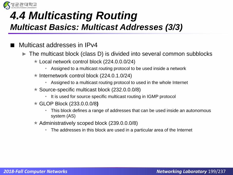
2018-Fall Computer Networks Networking Laboratory 199/237
4.4 Multicasting Routing Multicast Basics: Multicast Addresses (3/3)
Multicast addresses in IPv4
► The multicast block (class D) is divided into several common subblocks
Local network control block (224.0.0.0/24)
• Assigned to a multicast routing protocol to be used inside a network
Internetwork control block (224.0.1.0/24)
• Assigned to a multicast routing protocol to used in the whole Internet
Source-specific multicast block (232.0.0.0/8)
• It is used for source specific multicast routing in IGMP protocol
GLOP Block (233.0.0.0/8)
• This block defines a range of addresses that can be used inside an autonomous
system (AS)
Administratively scoped block (239.0.0.0/8)
• The addresses in this block are used in a particular area of the Internet

2018-Fall Computer Networks Networking Laboratory 200/237
4.4 Multicasting Routing Multicast Basics: Collecting groups information(1/3)
IGMP: Internet Group Management Protocol
► The protocol that is used today for collecting information about group
membership
► IGMP is a protocol defined at the network layer
► IGMP messages are encapsulated in an IP datagram
► There are only two types of messages in IGMP version3
Query and report messages
[ Fig 4.95 IGMP operation ]

2018-Fall Computer Networks Networking Laboratory 201/237
4.4 Multicasting Routing Multicast Basics: Collecting groups information(2/3)
IGMP
► Query message:
A query message is periodically sent by a router to all hosts attached to it to ask
them to report their interests about membership in groups. It can take one of
three forms:
1. A general query message is sent about membership in any group
• It is encapsulated in a datagram with the destination address 224.0.0.1
• All routers attached to the same network receive this message to inform them that this
message is already sent and that they should refrain from resending it
2. A group-specific query message is sent from a router to ask about the
membership related to a specific group
• This is sent when a router does not receive a response about a specific group and
wants to be sure that there is no active member of that group in the network

2018-Fall Computer Networks Networking Laboratory 202/237
4.4 Multicasting Routing Multicast Basics: Collecting groups information(3/3)
IGMP
► Query message
3. A source-and-group-specific query message is sent from a router to ask about
the membership related to a specific group when the message comes from a
specific source or sources
► Report message
A report message is sent by a host as a response to a query message
The message contains a list of records in which each record gives the identifier
of the corresponding group and the addresses of all sources that the host is
interested in receiving messages from
The message is encapsulated in a datagram with the multicast address
224.0.0.22

2018-Fall Computer Networks Networking Laboratory 203/237
4.4 Multicasting Routing Multicast Basics: Multicast forwarding (1/2)
Multicast forwarding
► In unicast communication, the destination address of the packet defines one
single destination
► In multicast communication, the destination of the packet defines one
group, but that group may have more than one member in the internet
[ Fig 4.96 Destination in unicasting and multicasting ]

2018-Fall Computer Networks Networking Laboratory 204/237
4.4 Multicasting Routing Multicast Basics: Multicast forwarding (2/2)
Multicast forwarding
► Forwarding in unicast communication depends only on the destination
address of the packet
► Forwarding decisions in multicast communication depend on both the
destination and the source address of the packet
Forwarding is based on where the packet should go and where the packet has
come from
[ Fig 4.97 Forwarding depends on the destination and the source ]

2018-Fall Computer Networks Networking Laboratory 205/237
Practice Problem
Difference between multicast and unicast forwarding

2018-Fall Computer Networks Networking Laboratory 206/237
4.4 Multicasting Routing Multicast Basics: Two approaches to multicasting
Two approaches to multicasting
► Source-based tree: one tree per source
shortest path trees
reverse path forwarding
► Group-shared tree: group uses one tree
minimal spanning (Steiner)
center-based trees

2018-Fall Computer Networks Networking Laboratory 207/237
4.4 Multicasting Routing Intradomain Routing Protocol: DVMRP (1/3)
Multicast Distance Vector (Distance Vector Multicast Routing Protocol -
DVMRP) is the extension of the RIP which is used in unicast routing. It
uses the source-based tree approach to multicasting in three steps:
► The router uses an algorithm called Reverse Path Forwarding (RPF)
► The router uses an algorithm called Reverse Path Broadcasting (RPB)
► The router uses an algorithm called Reverse Path Multicasting (RPM)

2018-Fall Computer Networks Networking Laboratory 208/237
4.4 Multicasting Routing Intradomain Routing Protocol: DVMRP (2/3)
Reverse Path Forwarding (RPF)
► It relies on router’s knowledge of unicast shortest path from the source
to the router
Reverse Path Broadcasting (RPB)
► RPB actually creates a broadcast tree from the graph that has been created
by the RPF algorithm
[ Fig 4.98 RPF versus RPB ]

2018-Fall Computer Networks Networking Laboratory 209/237
4.4 Multicasting Routing Intradomain Routing Protocol: MOSPF (1/2)
Multicast Link State (Multicast Open Shortest Path First -MOSPF)
► It is the extension of the OSPF protocol, which is used in unicasting routing
The router uses the Dijkstra algorithm to create a shortest-path tree with S as the
root and all destination in the internet as the leaves
The router finds itself in the shortest-path tree created in the first step
The shortest-path subtree is actually a broadcast subtree with the router as the
root and all networks as the leaves
The router can forward the received packet out of only those interfaces that
correspond to the branches of the multicast tree

2018-Fall Computer Networks Networking Laboratory 210/237
4.4 Multicasting Routing Intradomain Routing Protocol: MOSPF (2/2)
Multicast Open Shortest Path First (MOSPF)
[ Fig 4.99 Example of tree formation in MOSPF ]

2018-Fall Computer Networks Networking Laboratory 211/237
4.4 Multicasting Routing Intradomain Routing Protocol: PIM (1/4)
Protocol Independent Multicast (PIM)
► Not dependent on any specific underlying unicast routing algorithm (works
with all)
► Two different multicast distribution scenarios
Protocol Independent Multicast-Dense Mode (PIM-DM)
• Group members densely packed, in “close” proximity.
• Bandwidth more plentiful
Protocol Independent Multicast-Sparse Mode (PIM-SM)
• Group members “widely dispersed”
• Bandwidth not plentiful

2018-Fall Computer Networks Networking Laboratory 212/237
4.4 Multicasting Routing Intradomain Routing Protocol: PIM (2/4)
Protocol Independent Multicast (PIM)
► PIM-DM: The first packet is broadcast to all networks, which have or do not
have members. After a prune message arrives from a router with no
member, the second packet is only multicast.
[ Fig 4.100 Idea behind PIM-DM ]

2018-Fall Computer Networks Networking Laboratory 213/237
4.4 Multicasting Routing Intradomain Routing Protocol: PIM (3/4)
Protocol Independent Multicast (PIM)
► PIM-SM: The core router in PIM-SM is called the rendezvous point (RP).
Multicast communication is achieved in two steps:
Any router that has a multicast packet to send to a group of
destinations first encapsulates the multicast packet in a unicast packet
(tunneling) and sends it to the RP.
The RP then decapsulates the unicast packet and sends the multicastpacket to
its destination.

2018-Fall Computer Networks Networking Laboratory 214/237
4.4 Multicasting Routing Intradomain Routing Protocol: PIM (4/4)
Protocol Independent Multicast (PIM)
[ Fig 4.101 Idea behind PIM-SM ]

2018-Fall Computer Networks Networking Laboratory 215/237
4.5 Internet Protocol version 6 Introduction: Internet Protocol version 6 (IPv6)
An IPv6 address is 128 bits long. Compared with the 32-bit address of
IPv4, this is a huge (296 times) increase in the address space
The main changes in the IPv6 protocol:
► Larger address space.
► Better header format: IPv6 uses a new header format in which options are
separated from the base header and inserted. This simplifies and speeds up
the routing process because most of the options do not need to be checked
by routers
► New options: IPv6 has new options to allow for additional functionalities
► Allowance for extension: to allow the extension of the protocol if required by
new technologies or applications
► Support for resource allocation: two new fields, traffic class and flow label,
have been added to enable the source to request special handling of the
packet. E.g. support traffic such as real-time audio and video
► Support for more security: providing the encryption and authentication options

2018-Fall Computer Networks Networking Laboratory 216/237
4.5 Internet Protocol version 6 Introduction: Video (1/2)
Video Content
► When the Internet was launched in 1983, no one ever dreamed that there
might be billions of devices and users trying to get online
► But like a telephone network that is running out of phone numbers, the
current Internet is running out of IP addresses
► And if we don't roll out Internet Protocol v6 (IPv6), we won't have the room
we need to grow and the Internet would become tangled, unsafe and
unsustainable
► Link: https://www.youtube.com/watch?v=-Uwjt32NvVA

2018-Fall Computer Networks Networking Laboratory 217/237
4.5 Internet Protocol version 6 Introduction: Video (1/2)
https://www.youtube.com/watch?v=-Uwjt32NvVA

2018-Fall Computer Networks Networking Laboratory 218/237
4.5 Internet Protocol version 6 Packet Format (1/4)
[ Fig 4.101 IPv6 datagram ]

2018-Fall Computer Networks Networking Laboratory 219/237
4.5 Internet Protocol version 6 Packet Format (2/4)
Version: For IPv6, the value is 6
Traffic class: Identify priority among datagrams in flow. It replaces the
type-of-service field in IPv4.
Flow Label: Identify datagrams in same “flow”
Payload length: 2-byte payload length field defines the length of the IP
datagram excluding the header
Next header: Identify upper layer protocol or the type of first
extensionheader
Hop limit: The 8-bit hop limit field serves the same purpose as the TTL
field in IPv4
Source and destination address: These are 16-byte field which defines
Internet address of the source and destination
Payload: the payload field in IPv6 has a different format and meaning

2018-Fall Computer Networks Networking Laboratory 220/237
4.5 Internet Protocol version 6 Packet Format (3/4)
Payload: the payload field in IPv6 has a different format and meaning
[ Fig 4.102 Payload in an IPv6 datagram ]

2018-Fall Computer Networks Networking Laboratory 221/237
4.5 Internet Protocol version 6 Packet Format (4/4)
Concept of flow and priority in IPv6
► In IPv6, the flow label has been directly added to the format of the IPv6
datagram to allow us to use IPv6 as a connection-oriented protocol
Fragmentation and reassembly
► IPv6 datagrams can be fragmented only by the source, not by the routers
► The reassembly takes place at the destination
Extension headers
► Extension headers play a necessary and important part in IPv6. In
particular, three extension headers - fragmentation, authentication, and
extended security payload - are present in some packets.

2018-Fall Computer Networks Networking Laboratory 222/237
4.5 Internet Protocol version 6 IPv6 Addressing
An IPv6 address is 128 bits or 16 bytes long, four times the address
length in IPv4
Binary : 1111111011110110 ……... 1111111100000000
Colon hexadecimal : FEF6:BA98:7654:3210:ADEF:BBFF:2922:FF00
The leading zeros of a section can be omitted
0074 74, 000F F
Zero compression
FDEC:0:0:0:0:BBFF:0:FFFF FEDC::BBFF:0:FFFF

2018-Fall Computer Networks Networking Laboratory 223/237
4.5 Internet Protocol version 6 IPv6 Addressing
IPv6 uses hierarchical addressing
IPv6 allows slash or CIDR notation
Address space
► The address space of IPv6 contains 2128 addresses
► This address space is 296 times the IPv4 address
Three address types
► Unicast
► Anycast
► Multicast

2018-Fall Computer Networks Networking Laboratory 224/237
4.5 Internet Protocol version 6 IPv6 Addressing: Address space allocation(1/3)
The address space of IPv6 is divided into several blocks of varying size
and block is allocated for a special purpose
[ Table 4.7 Prefixes for assigned IPv6 addresses ]

2018-Fall Computer Networks Networking Laboratory 225/237
4.5 Internet Protocol version 6 IPv6 Addressing: Address space allocation(2/3)
Global unicast addresses
[ Fig 4.103 Global unicast address ]

2018-Fall Computer Networks Networking Laboratory 226/237
4.5 Internet Protocol version 6 IPv6 Addressing: Address space allocation(3/3)
The block in global unicast addresses is used for unicast
communication between two hosts in the Internet
The global routing prefix is used to route the packet through the Internet
to the organization site, such as the ISP that owns the block
The last q bits define the interface identifier

2018-Fall Computer Networks Networking Laboratory 227/237
4.5 Internet Protocol version 6 IPv6 Addressing: Special addresses (1/4)
The unspecified address is a subblock containing only one single
address, which is used during bootstrap when a host does not know its
own address and wants to send inquiry to find it
The loopback address consists of one single address

2018-Fall Computer Networks Networking Laboratory 228/237
4.5 Internet Protocol version 6 IPv6 Addressing: Special addresses (2/4)
A compatible address is used when a computer using IPv6 wants to
send a message to another computer using IPv6
A mapped address is used when a computer already migrated to
version 6 wants to send an address to a computer still using version 4

2018-Fall Computer Networks Networking Laboratory 229/237
4.5 Internet Protocol version 6 IPv6 Addressing: Special addresses (3/4)
Other Assigned Blocks
► IPv6 uses two large blocks for private addressing and one large block for
multicasting
► Unique local block
The packet carrying this type of address as the destination address is not
expected to be routed
► Link local block
It is designed for private addresses

2018-Fall Computer Networks Networking Laboratory 230/237
4.5 Internet Protocol version 6 IPv6 Addressing: Special addresses (4/4)
Other Assigned Blocks
► Multicast block
It is used to define a group of hosts instead of just one

2018-Fall Computer Networks Networking Laboratory 231/237
4.5 Internet Protocol version 6 Transition from IPv4 to IPv6: Dual stack
It is recommended that all hosts before migrating completely to version
6, have a dual stack of protocols during the transition
[ Fig 4.106 Dual stack ]

2018-Fall Computer Networks Networking Laboratory 232/237
4.5 Internet Protocol version 6 Transition from IPv4 to IPv6: Tunneling
Tunneling is a strategy used when two computers using IPv6 want to
communicate with each other and the packet must pass through a
region that used IPv4
[ Fig 4.107 Tunneling strategy ]

2018-Fall Computer Networks Networking Laboratory 233/237
4.5 Internet Protocol version 6 Transition from IPv4 to IPv6: Header Translation
Header translation is necessary when the majority of the Internet has
moved to IPv6 but some systems still use IPv4
[ Fig 4.108 Header translation strategy ]

2018-Fall Computer Networks Networking Laboratory 234/237
Practice Problem
Why we are moving to IPv6

2018-Fall Computer Networks Networking Laboratory 235/237
4.5 Internet Protocol version 6 ICMPv6
ICMPv6 (Internet Control Message Protocol version 6)
► This new version follows the same strategy and purposes of version 4
► It is more complicated than ICMPv4
Some protocols that were independent in version 4 are now part of ICMPv6
Some new messages have been added to make it more useful
[ Fig 4.109 Comparison of network layer in version 4 and version 6 ]

2018-Fall Computer Networks Networking Laboratory 236/237
4.5 Internet Protocol version 6 ICMPv6: Types of ICMPv6 (1/2)
[ Fig 4.110 ICMPv6 messages (part 1) ]

2018-Fall Computer Networks Networking Laboratory 237/237
[ Fig 4.110 ICMPv6 messages (part 2) ]
4.5 Internet Protocol version 6 ICMPv6: Types of ICMPv6 (2/2)