chapter 4 fundamentals of probability, random processes ... · fundamentals of probability, random...

“book˙uq”2013/9/5page 69i

ii

i

ii

ii

Chapter 4

Fundamentals ofProbability, RandomProcesses and Statistics

We summarize in this chapter those aspects of probability, random processes andstatistics that are employed in subsequent chapters. The discussion is necessarilybrief and additional details can be found in the references cited both in the textand noted in Section 4.9.

4.1 Random Variables, Distributions and DensitiesWhen constructing statistical models for physical and biological processes, we willconsider parameters and measurement errors to be random variables whose statis-tical properties or distributions we wish to infer using measured data. The classicalprobability space provides the basis for defining and illustrating these concepts.

Definition 4.1 (Probability Space). A probability space (⌦,F , P ) is comprisedof three components:

⌦: sample space is the set of all possible outcomes from an experiment;

F : �-field of subsets of ⌦ that contains all events of interest;

P : F ! [0, 1]: probability or measure that satisfies the postulates

(i) P (;) = 0,

(ii) P (⌦) = 1,

(iii) if Ai 2 F and Ai \ Aj = ;, then P (S1

i=1

Ai) =P1

i=1

P (Ai).

We note that the concept of probability depends on whether one is consideringa frequentist (classical) or Bayesian perspective. In the frequentist view, probabil-ities are defined as the frequency with which an event occurs if the experiment isrepeated a large number of times. The Bayesian perspective treats probabilities as adistribution of subjective values, rather than a single frequency, that are constructedor updated as data is observed.

69


ii

i

ii

ii

70 Chapter 4. Fundamentals of Probability, Random Processes and Statistics

Example 4.2. Consider an experiment in which we flip two individual coins (e.g.,a quarter and nickel) multiple times and record the outcome which consists of anordered pair. The sample space and �-field of events are thus

⌦ = {(H, H), (T, H), (H, T ), (T, T )}F = {;, (H, H), (T, H), (H, T ), (T, T ), ⌦, {(H, T ), (T, H), · · · }}.

(4.1)

Note that F contains all countable intersections and unions of elements in ⌦. If weflip the pair twice, two possible events are

A = {(H, H), (T, H)} , B = {(H, H), (H, T )} .

For fair coins, the frequentist perspective yields the probabilities

P (A) =1

2, P (B) =

1

2, P (A \ B) =

1

4, P (A [ B) =

3

4.

We note that because the events are independent, P (A\B) = P (A)P (B). We willrevisit the probabilities associated with flipping a coin from the Bayesian perspectivein Example 4.66 of Section 4.8.2.

We now define univariate random variables, distributions and densities.

4.1.1 Univariate Concepts

Definition 4.3 (Random Variable). A random variable is a function X : ⌦ ! Rwith the property that {! 2 ⌦|X(!) x} 2 F for each x 2 R; i.e., it is measurable.A random variable is said to be discrete if it takes values in a countable subset{x

1

, x2

, · · · } of R.

Definition 4.4 (Realization). The value

x = X(!)

of a random variable X for an event ! 2 ⌦ is termed a realization of X.

We note that in the statistics literature, many authors employ the same nota-tion for the random variable and realization and let the context dictate the meaning.For those who are new to the field, this can obscure the meaning and, to the degreepossible, we will use di↵erent notation for random variables and their realizations.

Definition 4.5 (Cumulative Distribution Function). Associated with everyrandom variable X is a cumulative distribution function (cdf) FX : R ! [0, 1] givenby

FX(x) = P{! 2 ⌦|X(!) x}. (4.2)

This is often expressed as FX(x) = P{X x} which should be interpreted inthe sense of (4.2). The following example illustrates the construction of a cdf for adiscrete random variable.


ii

i

ii

ii

4.1. Random Variables, Distributions and Densities 71

Example 4.6. Consider the experiment of Example 4.2 in which our event ! con-sists of a single flip of a pair of coins. We define X(!) to be the number of headsassociated with the event so that

X(H, H) = 2

X(H, T ) = X(T, H) = 1

X(T, T ) = 0.

For x < 0, the probability of finding an event ! 2 ⌦ such that X(!) x is 0 soFX(x) = 0 for x < 0. Similar analysis yields the cdf relation

FX(x) =

8

>

>

<

>

>

:

0 x < 01/4 , 0 x < 13/4 , 1 x < 21 , x � 2

which is plotted in Figure 4.1.

It is observed that, by construction, the cdf satisfies the properties

(i) limx!�1

FX(x) = 0

(ii) x1

x2

) FX(x1

) FX(x2

)

(iii) limx!1

FX(x) = 1.

(4.3)

This is an example of a cadlag (French “continue a droite, limite a gauche) functionthat is right-continuous and has left limits everywhere. These functions also arisein stochastic processes that admit jumps.

For continuous and discrete random variables the probability density function(pdf) and probability mass function are defined as follows.

Definition 4.7 (Probability Density Function). The random variable X iscontinuous if its cumulative distribution function is absolutely continuous and hencecan be expressed as

FX(x) =

Z x

�1fX(s)ds , x 2 R

where the derivative fX = dFx

dx mapping R to [0,1) is called the probability densityfunction (pdf) of X.

(x)

1 2

1/4

3/4

1

x

FX

Figure 4.1. Cumulative distribution function for Example 4.6.


ii

i

ii

ii


Definition 4.8 (Probability Mass Function). The probability mass function ofa discrete random variable X is given by fX(x) = P (X = x).

The pdf properties

(i) fX(x) � 0

(ii)

Z

RfX(x)dx = 1

(iii) P (x1

X x2

) = FX(x2

) � FX(x1

) =

Z x2

x1

fX(x)dx

follow immediately from the definition and (4.3). The attributes of density functionscan be further specified by designating their location or centrality, their spread orvariability, their symmetry, and the contribution of tail behavior. In general, thisinformation is provided by moments

E(Xn) =

Z

RxnfX(x)dx

or central moments. For example, the mean

µ = E(X) =

Z

RxfX(x)dx,

also termed the first moment or expected value, provides a measure of the density’scentral location whereas the second central moment

�2 = var(X) = E[(X � µ)2] =

Z

R(x � µ)2fX(x)dx (4.4)

provides a measure of the density’s variability or width. This typically is termedthe variance of X and � is called the standard deviation. One often employs therelation

�2 = E(X2) � µ2

which results directly from (4.4). We note that the third moment (skewness) quanti-fies the density’s symmetry about µ whereas the fourth moment (kurtosis) quantifiesthe magnitude of tail contributions.

Important Distributions for Inference and Model Calibration

We summarize next properties of the univariate normal, uniform, chi-squared,Student’s t, beta, gamma, inverse-gamma and inverse chi-squared distributionswhich are important for frequentist and Bayesian inference and model calibration.

Definition 4.9 (Normal Distribution). In uncertainty quantification, a com-monly employed univariate density is the normal density

fX(x) =1

�p

2⇡e�(x�µ)2/2�2

, �1 < x < 1.


ii

i

ii

ii


The associated cumulative distribution function is

FX(x) =

Z x

�1f(s)ds =

1

2

1 + erf

✓

x � µ

�p

2

◆�

where the error function is defined to be

erf(x) =2p⇡

Z x

0

e�s2ds.

The notation X ⇠ N(µ, �2) indicates that the random variable X is normallydistributed with mean µ and variance �2. For the normal density, 68.29% of the areais within 1� of the mean µ and 95.45% is within 2� as illustrated in Figure 4.2(a).

Definition 4.10 (Continuous Uniform Distribution). A random variable Xis uniformly distributed on the interval [a, b], denoted X ⇠ U(a, b), if any value inthe interval is achieved with equal probability. The pdf and cdf are thus

fX(x) =1

b � a�[a,b](x) (4.5)

and

FX(x) =

8

<

:

0 , x < ax�ab�a , a x < b1 , x � b

(4.6)

where the characteristic function �[a,b](x) is defined to be unity on the interval [a, b]

and 0 elsewhere. The pdf is plotted in Figure 4.2(b). It is established in Exercise 4.1that the mean and variance of X are

E(X) =a + b

2, var(x) =

(b � a)2

12(4.7)

!1 !0.5 0 0.5 1 1.5 20

0.2

0.4

0.6

0.8

1

x

f(x)

1! 2!!1!!2!

34.1%34.1%

13.6%13.6%

a

b!a

1

x

f(x)

b

(a) (b)

Figure 4.2. (a) Normal density with µ = 0.5 and � = 0.4 and areas within 1� and2� of µ. (b) Uniform density on the interval [a, b].


ii

i

ii

ii


and the relationship between X ⇠ U(a, b) and Z ⇠ U(�1, 1) is established in Exer-cise 4.6. When prior information is lacking, it is often assumed that model param-eters have a uniform density.

Definition 4.11 (Chi-Squared Distribution). Let X ⇠ N(0, 1) be normallydistributed. The random variable Y = X2 then has a chi-squared distribution with1 degree of freedom, denoted Y ⇠ �2(1). Furthermore, if Yi, i = 1, · · · , k, are

independent �2(1) random variables, then their sum Z =Pk

i=1

Yi is a �2 randomvariable with k degrees of freedom, denoted Z ⇠ �2(k) or Z ⇠ �2

k. The probabilitydensity function

fZ(z; k) =

(

zk/2�1e�z/2

2

k/2�(k/2)

, z � 0

0 , z < 0(4.8)

can be compactly expressed in terms of the gamma function, where �(k/2) =p⇡ (k�2)!!

2

(k�1)/2 for odd k, and exhibits the behavior shown in Figure 4.3(a). The meanand variance of Z are

E(Z) = k , var(Z) = 2k.

Chi-squared distributions naturally arise when evaluating the sum of squares errorbetween measured data and model values when estimating model parameters.

Definition 4.12 (Student’s t-Distribution). Let X ⇠ N(0, 1) and Z ⇠ �2(k)be independent random variables. The random variable

T =X

p

Z/k

has a Student’s t-distribution (or simply t-distribution) with k degrees of freedom.

0 2 4 6 80

0.1

0.2

0.3

0.4

0.5

z

f Z(z;k

)

k=1 k=2 k=3 k=4 k=5

−4 −2 0 2 40

0.1

0.2

0.3

0.4

t

f T(t;k)

k=1 k=2 k=10 Normal

(a) (b)

Figure 4.3. (a) Chi-squared density for k = 1, · · · , 5 and (b) Student’s t-densitywith k = 1, 2, 10 compared with the normal density with µ = 0, � = 1.


ii

i

ii

ii


The probability density function can be expressed as

fT (t; k) =�((k + 1)/2)

�(k/2)p

k⇡

✓

1 +t2

k

◆�(k+1)/2

where � again denotes the gamma function. Note that

fT (t; 1) =1

⇡(1 + t2)

is a special case of the Cauchy distribution. As illustrated in Figure 4.3(b), thedensity is symmetric and bell-shaped, like the normal density, but exhibits heaviertails.

It will be shown in Section 7.2 that the t-distribution naturally arises whenestimating the mean of a population when the sample size is relatively small andthe population variance is unknown.

On a historic note, aspects of this theory were developed by William SealyGosset, an employee of the Guinness brewery in Dublin, in an e↵ort to select opti-mally yielding varieties of barley based on relatively small sample sizes. To improveperception following the recent disclosure of confidential information by another em-ployee, Gosset was only allowed to publish under the pseudonym “Student.” Theimportance of his work was advocated by both Karl Person and R.A. Fisher.

Definition 4.13 (Gamma Distribution). The gamma distribution is a two-parameter family with two common parameterizations: (i) shape parameter ↵ > 0and scale parameter � > 0 or (ii) shape parameter ↵ and inverse scale or rateparameter � = 1/�. We employ the second since the inverse-gamma distributionformulated in terms of ↵ and � is a conjugate prior for likelihoods associated withnormal distributions with known mean and unknown variance; see Example 4.69.For X ⇠ Gamma(↵, �), the density is

fX(x; ↵, �) =�↵

�(↵)x↵�1e��x , x > 0,

and the expected value and variance are E(X) = ↵/� and var(X) = ↵/�2.In MATLAB, random values from a gamma distribution can be generated

using the command gamrnd.m which uses the first parameterization based on theshape and scale parameters ↵ and �.

We point out that the one-parameter �2

k distribution with k degrees of freedomis a special case of the gamma distribution with ↵ = k

2

and � = 1

2

.

Definition 4.14 (Inverse-Gamma Distribution). If X has a gamma distribu-tion, then Y = X�1 has an inverse-gamma distribution with parameters that satisfy

X ⇠ Gamma(↵, �) , Y ⇠ Inv-gamma(↵, �). (4.9)

Hence the density is

fY (y; ↵, �) =�↵

�(↵)y�(↵+1)e��/y , y > 0,


ii

i

ii

ii


and the mean and variance are E(Y ) = �↵�1

for ↵ > 1 and var(Y ) = �2

(↵�1)

2(↵�2)

for ↵ > 2.As noted in Definition 4.13 and illustrated in Example 4.69, the inverse-

gamma distribution is the conjugate prior for normal likelihoods that are functionsof the variance. The equivalence (4.9) can be used to generate random inverse-gamma values using the MATLAB Statistics Toolbox command gamrnd.m. Sincex = gamrnd(↵, �) is parameterized in terms of the scale parameter, one would em-ploy the command y = gamrnd(↵, �), with � = 1/�, to generate realizations ofY ⇠ Inv-gam(↵, �). A technique to construct random realizations from the inverse-gamma distribution, if gamrnd.m is not available, is discussed at the end of thissection.

Definition 4.15 (Inverse Chi-Squared Distribution). The inverse chi-squareddistribution is a special case of Inv-gamma(↵, �) with ↵ = k

2

, � = 1

2

so the densityis

fY (y; k) =2�k/2

�(k/2)y�(k/2+1)e�1/2y

for y > 0. This reparameterization can facilitate manipulation of conjugate familieswhen constructing Bayesian posterior distributions.

Definition 4.16 (Beta Distribution). The random variable X ⇠ Beta(↵, �) hasa beta distribution if it has the density

fX(x; ↵, �) =�(↵ + �)

�(↵)�(�)x↵�1(1 � x)��1

for x 2 [0, 1]. As illustrated in Example 4.68, it is the conjugate prior for the bino-mial likelihood. It is observed that if ↵ = � = 1, the beta distribution is simply theuniform distribution which is often used to provide noninformative priors. Realiza-tions from the beta distribution can be generated using the MATLAB commandbetarnd.m.

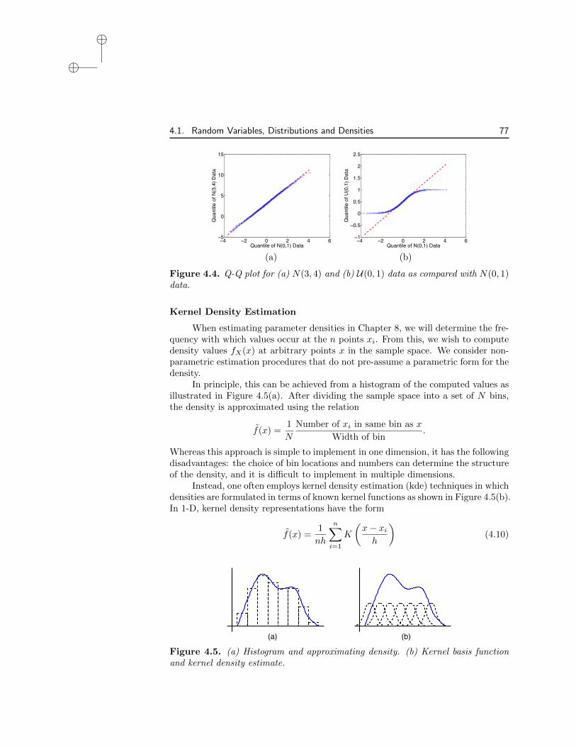
Definition 4.17 (Quantile-Quantile (Q-Q) Plots). A Q-Q plot is a graphi-cal method for comparing data from two distributions by plotting their quantilesagainst each other. We will typically use this to determine the degree to which datais Gaussian but the technique can be used to compare any distributions. If distri-butions are linearly related, Q-Q plots will be approximately linear. In MATLAB,Q-Q plots can be generated using the command qqplot.m.

To illustrate, we compare in Figure 4.4 realizations from N(3, 4) and U(0, 1)distributions with data from a N(0, 1) distribution. The linearity in the first caseillustrates that the two are from the same family whereas the quantiles di↵er sig-nificantly in the comparison between the uniform and normal data.


ii

i

ii

ii


−4 −2 0 2 4 6−5

0

5

10

15

Quantile of N(0,1) Data

Qua

ntile

of N

(3,4

) Dat

a

−4 −2 0 2 4 6−1

−0.5

0

0.5

1

1.5

2

2.5

Quantile of N(0,1) Data

Qua

ntile

of U

(0,1

) Dat

a

(a) (b)

Figure 4.4. Q-Q plot for (a) N(3, 4) and (b) U(0, 1) data as compared with N(0, 1)data.

Kernel Density Estimation

When estimating parameter densities in Chapter 8, we will determine the fre-quency with which values occur at the n points xi. From this, we wish to computedensity values fX(x) at arbitrary points x in the sample space. We consider non-parametric estimation procedures that do not pre-assume a parametric form for thedensity.

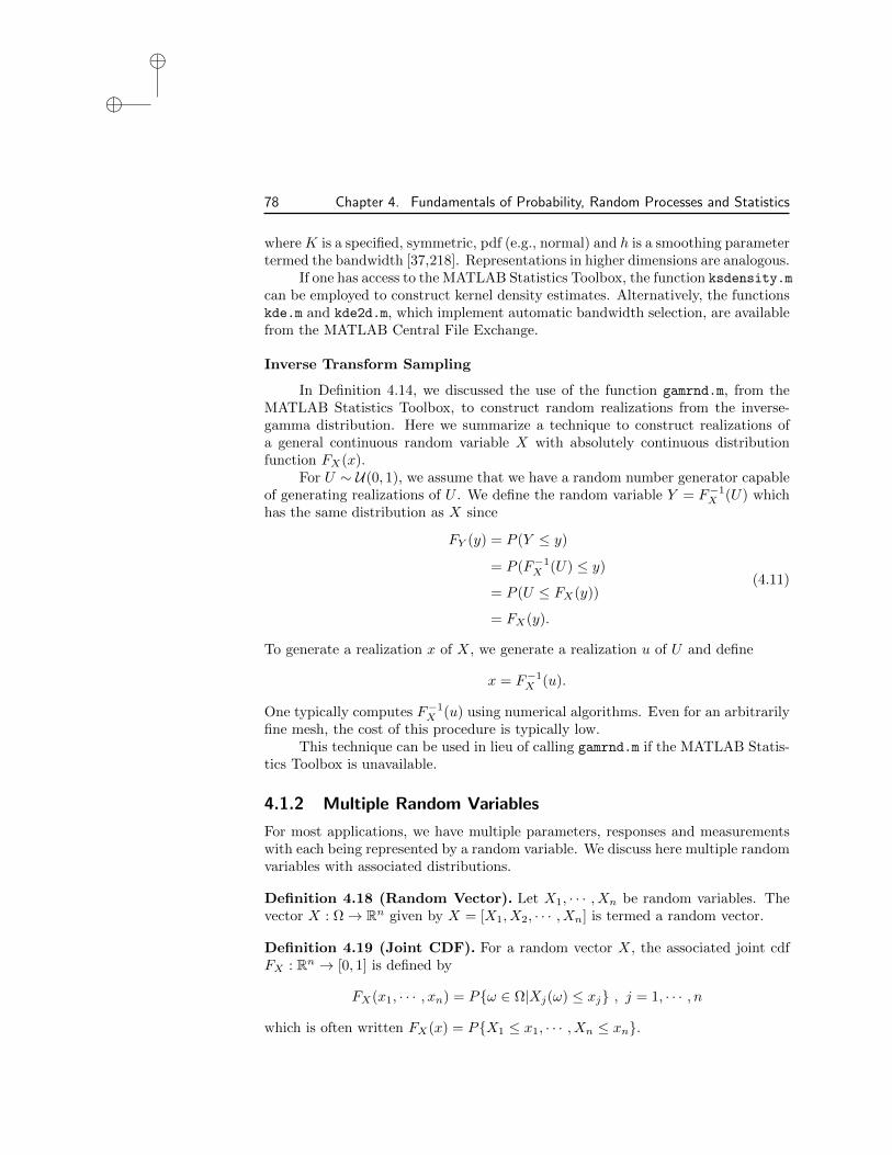
In principle, this can be achieved from a histogram of the computed values asillustrated in Figure 4.5(a). After dividing the sample space into a set of N bins,the density is approximated using the relation

f(x) =1

N

Number of xi in same bin as x

Width of bin.

Whereas this approach is simple to implement in one dimension, it has the followingdisadvantages: the choice of bin locations and numbers can determine the structureof the density, and it is di�cult to implement in multiple dimensions.

Instead, one often employs kernel density estimation (kde) techniques in whichdensities are formulated in terms of known kernel functions as shown in Figure 4.5(b).In 1-D, kernel density representations have the form

f(x) =1

nh

nX

i=1

K

✓

x � xi

h

◆

(4.10)

(b)(a)

Figure 4.5. (a) Histogram and approximating density. (b) Kernel basis functionand kernel density estimate.


ii

i

ii

ii


where K is a specified, symmetric, pdf (e.g., normal) and h is a smoothing parametertermed the bandwidth [37,218]. Representations in higher dimensions are analogous.

If one has access to the MATLAB Statistics Toolbox, the function ksdensity.m

can be employed to construct kernel density estimates. Alternatively, the functionskde.m and kde2d.m, which implement automatic bandwidth selection, are availablefrom the MATLAB Central File Exchange.

Inverse Transform Sampling

In Definition 4.14, we discussed the use of the function gamrnd.m, from theMATLAB Statistics Toolbox, to construct random realizations from the inverse-gamma distribution. Here we summarize a technique to construct realizations ofa general continuous random variable X with absolutely continuous distributionfunction FX(x).

For U ⇠ U(0, 1), we assume that we have a random number generator capableof generating realizations of U . We define the random variable Y = F�1

X (U) whichhas the same distribution as X since

FY (y) = P (Y y)

= P (F�1

X (U) y)

= P (U FX(y))

= FX(y).

(4.11)

To generate a realization x of X, we generate a realization u of U and define

x = F�1

X (u).

One typically computes F�1

X (u) using numerical algorithms. Even for an arbitrarilyfine mesh, the cost of this procedure is typically low.

This technique can be used in lieu of calling gamrnd.m if the MATLAB Statis-tics Toolbox is unavailable.

4.1.2 Multiple Random Variables

For most applications, we have multiple parameters, responses and measurementswith each being represented by a random variable. We discuss here multiple randomvariables with associated distributions.

Definition 4.18 (Random Vector). Let X1

, · · · , Xn be random variables. Thevector X : ⌦ ! Rn given by X = [X

1

, X2

, · · · , Xn] is termed a random vector.

Definition 4.19 (Joint CDF). For a random vector X, the associated joint cdfFX : Rn ! [0, 1] is defined by

FX(x1

, · · · , xn) = P{! 2 ⌦|Xj(!) xj} , j = 1, · · · , n

which is often written FX(x) = P{X1

x1

, · · · , Xn xn}.


ii

i

ii

ii


Consider now the random variables X1

, · · · , Xn each having an expectationE(Xi). It follows immediately that

E

nX

i=1

aiXi

!

=nX

i=1

aiE(Xi) (4.12)

where a1

, · · · , an are real constants. Furthermore, if the n random variables areindependent, then

E(X1

X2

· · ·Xn) = E(X1

)E(X2

) · · ·E(Xn). (4.13)

Definition 4.20 (Covariance and Correlation). The covariance of random vari-ables X and Y is the number

cov(X, Y ) = E[(X � E(X))(Y � E(Y ))] = E(XY ) � E(X)E(Y ) (4.14)

and the correlation or correlation coe�cient is

⇢XY =cov(X, Y )

�X�Y. (4.15)

We note that if X and Y are independent, then cov(X, Y ) = ⇢XY = 0 and therandom variables are uncorrelated. The converse is not true in general since therelation (4.15) quantifies only linear dependencies among random variables.

Returning to the case of n random variables, it is shown in [95] that

var

nX

i=1

aiXi

!

=nX

i=1

a2

i var(Xi) + 2X

i<j

aiajcov(Xi, Xj) (4.16)

which simplifies to

var

nX

i=1

aiXi

!

=nX

i=1

a2

i var(Xi) (4.17)

if the random variables are pairwise uncorrelated.

Theorem 4.21. Let X1

, · · · , Xn be mutually independent, normally distributed,random variables with Xi ⇠ N(µi, �2

i ) and let a1

, · · · , an and b1

, · · · , bn be fixedconstants. As proven in Corollary 4.6.2 of [60], it then follows that

Z =nX

i=1

(aiXi + bi) ⇠ N

nX

i=1

(aiµi + bi),nX

i=1

a2

i�2

i

!

. (4.18)

Like the univariate normal, the multivariate normal distribution plays a centralrole in uncertainty quantification and model validation.


ii

i

ii

ii


Definition 4.22 (Multivariate Normal Distribution). The random n-vectorX is said to be normally distributed with mean µ = [µ

1

, · · · , µn] and covariancematrix

V =

2

6

6

6

4

var(X1

) cov(X1

, X2

) · · · cov(X1

, Xn)cov(X

2

, X1

) var(X2

) · · · cov(X2

, Xn)...

......

cov(Xn, X1

) cov(Xn, X2

) · · · var(Xn)

3

7

7

7

5

, (4.19)

designated X ⇠ N(µ, V ), if the associated density is

fX(x) =1

p

(2⇡)n|V |exp

�1

2(x � µ)V �1(x � µ)T

�

.

Here x = [x1

, x2

, · · · , xn] and |V | is the determinant of V .

We use the next theorem when constructing proposal functions for the MCMCalgorithms detailed in Chapter 8.

Theorem 4.23. Let Y = [Y1

, · · · , Yn]T be a normally distributed random vector,Y ⇠ N(µ, V ), where V is positive definite. Let Z ⇠ N(0, In) where In is the n ⇥ nidentity. Then Y = (RZ + µ) where V = RRT and R is a lower triangular matrix.

A proof of this theorem can be found in [95]. We note that the decompositionV = RRT can be e�ciently computed using a Cholesky decomposition.

Finally, the concepts of marginal and conditional distributions and densitieswill play an important role in statistical inference. We summarize the definitionsfor continuous random variables and refer the reader to [110, 168] for analogousdefinitions for discrete random variables.

Definition 4.24 (Marginal PDF). Let X1

and X2

be jointly continuous randomvariables with joint pdf fX(x

1

, x2

). The marginal density functions of X1

and X2

are respectively given by

fX1(x

1

) =

Z

RfX(x

1

, x2

)dx2

, fX2(x

2

) =

Z

RfX(x

1

, x2

)dx1

.

A representative marginal density is plotted in Figure 4.6(a). Similarly for jointlycontinuous random variables X

1

, · · · , Xn with joint density function fX(x1

, · · · , xn),the marginal pdf of X

1

is

fX1(x1

) =

Z

R· · ·Z

RfX(x

1

, x2

, · · · , xn)dx2

· · · dxn.

Definition 4.25 (Conditional PDF). Let X1

and X2

be jointly continuous ran-dom variables with joint pdf fX(x

1

, x2

) and marginal pdf fX1(x

1

) and fX2(x

2

). Theconditional density of X

1

given X2

= x2

is

fX1|X2(x

1

|x2

) =

(

fX(x1,x2)

fX2(x2)

, fX2(x2

) > 0

0 , otherwise


ii

i

ii

ii

4.2. Estimators, Estimates and Sampling Distributions 81

(a) (b)

Figure 4.6. (a) Marginal density fX2(x2

) and (b) conditional density fX1|X2(x

1

|x2

)at x

2

= � 1

2

for a normal joint density fX(x1

, x2

) with covariance matrix V = 0.09I.

as plotted in Figure 4.6(b). We note that fX1|X2(x

1

|x2

) is a function of x1

. Thedefinition for fX2|X1

(x2

|x1

) is analogous. Similarly, for n jointly continuous ran-dom variables X

1

, · · · , Xn with joint density function fX(x1

, · · · , xn) and marginaldensity fX1

(x1

), the conditional pdf of X2

, · · · , Xn given X1

= x1

is

fX2,··· ,Xn|X1(x

2

, · · · , xn|x1

) =fX(x

1

, x2

, · · · , xn)

fX1(x1

).

Definition 4.26 (iid Random Variables). Random variables X1

, · · · , Xn aresaid to be independent and identically distributed (iid) with pdf f(x) if they aremutually independent and the marginal pdf fXi

for each Xi is the same functionf(x) = fX1

(x) = · · · fXn(x). The joint pdf for iid random variables is

fX(x1

, · · ·xn) =nY

i=1

f(xi). (4.20)

4.2 Estimators, Estimates and Sampling DistributionsIn this section, we summarize concepts pertaining to the estimation of unknownparameters through samples, observations, or measurements. In Section 4.3, we willdetail specific techniques to estimate parameters in the context of model calibration.More general theory pertaining to frequentist and Bayesian inference is provided inSection 4.8.

Definition 4.27 (Point and Interval Estimates). Consider a fixed but unknownparameter q 2 Q ⇢ Rp. A point estimate is a vector in Rp that represents q. Aninterval estimate provides an interval that quantifies the plausible location of com-ponents of q. The mean, median, or mode of a sampling distribution are examplesof point estimates whereas confidence intervals are interval estimates.


ii

i

ii

ii


Definition 4.28 (Estimator and Sampling Distribution). An estimator is arule or procedure that specifies how to construct estimates for q based on randomsamples X

1

, · · · , Xn. Hence the estimator is a random variable with an associateddistribution, termed the sampling distribution, which quantifies attributes of theestimation process. The estimate is a realization of the estimator so it is a functionof the realized values x

1

, · · · , xn. An estimator is said to be unbiased if its meanis equal to the value of the parameter being estimated. Otherwise it is said to bebiased. Two estimators that we will employ for model calibration are ordinary leastsquares and maximum likelihood estimators. We will also employ mean, varianceand interval estimators at various points in the discussion.

Definition 4.29 (Statistic). A statistic is a measurable function of one or morerandom variables that does not depend on unknown parameters.

Example 4.30. Let X1

, · · · , Xn be random variables associated with a sample ofsize n. Suppose we wish to estimate the population mean µ and variance �2 whichare assumed unknown. This can be accomplished using the estimators, or statistics,

X =1

n

nX

i=1

Xi , S2 =1

n � 1

nX

i=1

(Xi � X)2 (4.21)

which are the sample mean and variance. We note that we employ n�1 rather thann in the expression for S2 to ensure that it is unbiased. If we additionally assumethat Xi ⇠ N(µ, �2), it is illustrated in [168] that the sampling distributions for Xand S2 are

X ⇠ N

✓

µ,�2

n

◆

, S2 ⇠ �2

n � 1�2(n � 1). (4.22)

Definition 4.31 (Interval Estimator and Confidence Interval). The goalwhen constructing an interval estimate is to determine functions qL(x) and qR(x)that bound the location qL(x) < q < qR(x) of q based on realizations x = [x

1

, · · · , xn]of a random sample X = [X

1

, · · · , Xn]. The random interval [qL(X), qR(X)] istermed an interval estimator. An interval estimator in combination with a confi-dence coe�cient is commonly called a confidence interval. The confidence coe�cientcan be interpreted as the frequency of times, in repeated sampling, that the intervalwill contain the target parameter q. The (1 � ↵) ⇥ 100% confidence interval is thepair of statistics (qL(X), qR(X)) such that for all q 2 Q,

P [qL(X) q qR(X)] = 1 � ↵. (4.23)

Example 4.32. Consider a sequence of n random variables X1

, · · · , Xn from anormal distribution with known variance �2 and unknown mean µ; that is, Xi ⇠N(µ, �2). To determine information about the unknown mean, we consider thesample mean X given by (4.21) which has the sampling distribution given in (4.22).


ii

i

ii

ii

4.2. Estimators, Estimates and Sampling Distributions 83

It thus follows that¯X�µ�/

pn⇠ N(0, 1) so that

P

✓

�2 <X � µ

�/p

n< 2

◆

⇡ 0.9545

since 95.45% of the area of a normal distribution lies within 2 standard deviationsof the mean. This implies that

P

✓

X � 2�pn

< µ < X +2�p

n

◆

⇡ 0.9545.

Here [X � 2�/p

n, X + 2�/p

n] is an interval estimator for µ where both endpointsare statistics since �2 is considered known. A (1� ↵)⇥ 100% confidence interval is[x� 2�/

pn, x+2�/

pn] where x = 1

n

Pni=1

xi is the realized sample mean based onn measurements, or realizations, xi of the random variables Xi.

Example 4.33. We now turn to the problem of determining the confidence intervalfor the mean µ of a normal distribution when the variance �2 is also unknown. Toestimate �2, we employ the statistic S2 given by (4.21) which has the �2 distribution(4.22). We thus have

X =

pn(X � µ)

�⇠ N(0, 1) , Z =

(n � 1)S2

�2

⇠ �2(n � 1)

so that the quotient

T =X

p

Z/(n � 1)=

pn(X � µ)

S

has a t-distribution with n�1 degrees of freedom; see Definition 4.12. To determinea (1 � ↵) ⇥ 100% confidence interval for a given value of n, we seek values a and bsuch that

P

✓

a <

pn(X � µ)

S< b

◆

= 1 � ↵.

In Figure 4.3(b), it is shown that the t-distribution is symmetric so that b = �awhich we denote by tn�1,1�↵/2 to reflect the n � 1 degrees of freedom and interval1 � ↵/2. It then follows that

P

✓

X �tn�1,1�↵/2Sp

n< µ < X +

tn�1,1�↵/2Spn

◆

= 1 � ↵.

On can employ standard tables of t-distributions to determine tn�1,1�↵/2 given ↵and n and thus specify the (1�↵)⇥100% confidence interval [X�tn�1,1�↵/2S/

pn ,

X + tn�1,1�↵/2S/p

n ]. We remind the reader that for ↵ = 0.05, this is a randominterval that has a 95% chance of containing the unknown but fixed (deterministic)parameter µ. The interval is constructed by obtaining measurements x

1

, · · · , xn andemploying the realizations x = 1

n

Pni=1

xi and s2 = 1

n�1

Pni=1

(xi � x)2 to obtain

x �tn�1,1�↵/2 sp

n, x +

tn�1,1�↵/2 spn

�

.


ii

i

ii

ii


We will use t-distributions in this manner in Chapter 7 to construct confidenceintervals for model parameters determined using least squares estimators when � isunknown and the degrees of freedom is relatively small.

4.3 Ordinary Least Squares and Maximum LikelihoodEstimators

The process of model calibration entails estimating model parameters, and pos-sibly initial and boundary conditions, based on measured data. More generally,the estimation of model parameters, based on observations, comprises a significantcomponent of statistical inference which is further discussed in Section 4.8.

To motivate, consider the statistical model

⌥i = f(ti, q0) + "i , i = 1, · · · , n (4.24)

where ⌥i are random variables whose realizations �i are a set of n measurementsfrom an experiment and f(ti, q) is the parameter-dependent model response orquantity of interest at corresponding times. The random variables "i account forerrors between the model and measurements. Finally, q

0

denotes the true, butunknown, parameter value that we cannot measure directly but instead must inferfrom realizations of the random variables ⌥i. We emphasize that in this context,q0

is not a random variable.

4.3.1 Ordinary Least Squares (OLS) Estimator

Consider (4.24) with the assumption that errors "i are independent and identi-cally distributed (iid), unbiased so E("i) = 0, and have true but unknown variancevar("i) = �2

0

. We assume that the true parameter q0

is in an admissible parameterspace Q and we let Q denote the corresponding sample space. As illustrated in theexamples of Chapter 7, these spaces typically coincide.

The ordinary least squares estimator and estimate1

qOLS = argminq2Q

nX

i=1

[⌥i � f(ti, q)]2

qOLS = argminq2Q

nX

i=1

[�i � f(ti, q)]2

(4.25)

are the random variable and realization in Rp that minimize the respective sum ofsquares errors as illustrated in Figure 4.7(a). Details regarding the distribution ofqOLS based on various assumptions regarding the distribution of the errors "i areprovided in Chapter 7.

1The use of the notation qOLS to indicate the estimator is not universal and many textsdenote the least squares estimate by the hat-notation. Hence care must be taken to establish theconvention employed in the specific text.


ii

i

ii

ii

4.3. Ordinary Least Squares and Maximum Likelihood Estimators 85

MLEq

(a)

qOLS

(b)

Figure 4.7. (a) Ordinary least squares solution qOLS to (4.25) and (b) maximumlikelihood estimate qMLE given by (4.27).

4.3.2 Maximum Likelihood Estimator (MLE)

Maximum likelihood estimators can also be used to achieve the objective of esti-mating a parameter q based on random samples ⌥

1

, · · · , ⌥n.

Definition 4.34 (Likelihood Function). Let f⌥

(�; q) be a parameter-dependentjoint pdf associated with a random vector ⌥ = [⌥

1

, · · · , ⌥n], where q 2 Q is anunknown parameter vector, and let � = [�

1

, · · · , �n] be a realization of ⌥. Thelikelihood function L : Q ! [0,1) is defined by

L�(q) = L(q|�) = f⌥

(�; q) (4.26)

where the observed sample � is fixed and q varies over all admissible parametervalues. The notation L�(q) is somewhat nonstandard but it highlights the fact thatthe independent variable is q. Some authors use the notation

L(q) = L(q|d) = f⌥

(d; q),

where d = [d1

, · · · dn] denotes the outcome from a random experiment, to reinforcethis concept.

We note that because L is function of q, it is not a probability density functionand the notation L(q|�), while standard, should not be interpreted as a conditionalpdf. If Y is discrete, then L�(q) is the probability of obtaining the data � for agiven parameter value q. For continuous ⌥, the fact that L is only defined to withina constant of proportionality can be combined with Riemann sum approximationsof the integral to obtain a similar interpretation.

For n iid random variables, it follows from (4.20) that the likelihood functionis

L(q|�) =nY

i=1

f⌥

(�i; q).

Finally, we denote the log-likelihood function by

`�(q) = `(q|�) = ln L(q|�).


ii

i

ii

ii


Example 4.35. Consider the binomial distribution with probability of success p.The probability mass function

f⌥

(�; p, n) = P (⌥ = �|n, p) =

✓

n�

◆

p�(1 � p)n�p

quantifies the probability of obtaining exactly � = 0, 1, · · · , n successes in a sequenceof n experiments. In this function, p and n are known and � is unknown. Althoughthe likelihood

L(q|�, n) =

✓

n�

◆

p�(1 � p)n�p

has the same functional form, the independent variable now is p, and � and n areknown. Hence the likelihood function is continuous whereas the probability massfunction is discrete.

Estimates for q0

are commonly constructed by computing the value of q thatmaximizes the likelihood which is termed a maximum likelihood estimate (MLE).For iid samples, the maximum likelihood estimate is

qMLE = argmaxq2Q

nY

i=1

f⌥

(�i|q).

To illustrate, we consider (4.24) with the assumption that errors are iid,unbiased, and normally distributed with true but unknown variance �2

0

so that"i ⇠ N(0, �2

0

) and hence ⌥i ⇠ N(f(ti, q0), �2

0

). In this case q and �2 are bothparameters so the likelihood function is

L(q, �|�) =nY

i=1

1

�p

2⇡e�[�i�f(ti,q)]

2/2�2

=1

(2⇡�2)n/2e�

Pni=1[�i�f(ti,q)]

2/2�2

(4.27)

and the maximum likelihood estimate is

qMLE = argmaxq2Q

�22(0,1)

L(q, �|�) (4.28)

as depicted in Figure 4.7(b).Due to the monotonicity of the logarithm function, maximizing L(q,�|�) is

equivalent to maximizing the log likelihood

`(q, �|�) = �n

2ln(2⇡) � n

2ln(�2) � 1

2�2

nX

i=1

[�i � f(ti, q)]2 .

From a computational perspective, however, the log likelihood is advantageous soit is commonly employed in algorithms. For fixed �2, the condition d

dq `(�|q, �) = 0yields

nX

i=1

[�i � f(ti, q)]rf(ti, q) = 0 (4.29)


ii

i

ii

ii

4.4. Modes of Convergence and Limit Theorems 87

where rf denotes the gradient of f with respect to q. It is observed that with theassumption of iid, unbiased, normally distributed errors, the maximum likelihoodsolution qMLE to (4.29) is the same as the least squares estimate qOLS specified by(4.25). The equivalence between minimizing the sum of squares error and maxi-mizing the likelihood will be utilized when we construct proposal functions for theMCMC techniques in Chapter 8.

In frequentist inference, the maximum likelihood estimate qMLE is the param-eter value that makes the observed output most likely. It should not be interpretedas the most likely parameter value resulting from the data since this would requireit to be a random variable which contradicts the tenets of frequentist analysis.

4.4 Modes of Convergence and Limit TheoremsThere are several modes of convergence for sequences of random variables and dis-tributions that are important for our discussion. We summarize the definitions andrefer the reader to [60, 80,81] for additional details, examples and proofs of relatedtheorems.

Definition 4.36 (Convergence in Probability). A sequence X1

, X2

, · · · of ran-

dom variables converges in probability to a random variable X, written as XnP! X,

if for every " > 0,

limn!1

P (|Xn � X| � ") = 0 or, equivalently, limn!1

P (|Xn � X| < ") = 1.

Note that X1

, X2

, · · · are typically not iid in this and following definitions. Thismode of convergence is weaker than almost sure convergence.

Definition 4.37 (Almost Sure Convergence). A sequence X1

, X2

, · · · of ran-dom variables converges almost surely to a random variable X, written Xn

a.s.�! X,if for every " > 0,

P⇣

limn!1

|Xn � X| < "⌘

= 1.

Examples of sequences that converge in probability but not almost surely are pro-vided in [60]. This is sometimes referred to as convergence with probability 1.

Definition 4.38 (Convergence in Distribution). Let X1

, X2

, · · · be a sequenceof random variables with corresponding distributions FX1

(x), FX2(x), · · · . If FX(x)

is a distribution function and

limn!1

FXn(x) = FX(x)

at all points x where FX(x) is continuous, then Xn is said to have a limiting randomvariable X with distribution function FX(x). In this case, Xn is said to converge

in distribution to X, which is often written as XnD! X. Care must be taken when

using this notation since the convergence of random variables is defined in terms


ii

i

ii

ii


of the convergence of the distributions. Hence this mode of convergence is quitedi↵erent from the previous two.

We note that almost sure convergence implies convergence in probability whichin turn implies convergence in distribution. Hence convergence in distribution is theweakest of the three concepts.

Definition 4.39 (Consistent Estimator). A sequence qn of estimators is saidto be consistent, or weakly consistent, if it converges in probability to the value q

0

of the parameter being estimated. In practice, we often construct estimators thatare a function of the sample size n. In this case, the estimator is consistent if thesequence converges in probability to q

0

as the number of samples tends to infinity.

Law of Large Numbers and Central Limit Theorem

The Law of Large Numbers and Central Limit Theorem are two of the pillarsof probability theory. To motivate them, we consider the problem of estimating theunknown mean µ and variance �2 of a population based on samples x

1

, x2

, · · · andassociated random variables X

1

, X2

, · · · . An estimator for the mean is

Xn =1

n

nX

i=1

Xi (4.30)

so a natural question is the following: Does limn!1 Xn = µ? This is addressed bythe strong and weak laws of large numbers.

Theorem 4.40 (Strong Law of Large Numbers). Let X1

, X2

, · · · be iid randomvariables with E(Xi) = µ and var(Xi) = �2 < 1 and define Xn by (4.30). Thenfor every " > 0,

P⇣

limn!1

|Xn � µ| < "⌘

= 1 or Xna.s.�! µ.

The formulation of the weak Law of Large Numbers is similar except XnP! µ.

These laws are of fundamental importance since they establish that the randomsample adequately represents the population in the sense that Xn converges to themean µ.

Given the central role of the sample mean, it is natural to question the degreeto which its sampling distribution can be established. In Example 4.30, we notedthat if Xi ⇠ N(µ, �2) then X ⇠ N(µ, �2/n). The requirement of normally dis-tributed random variables is quite restrictive, however, so we relax this assumptionand pose the same question in the context of iid random variables from an arbitrarydistribution. The remarkable answer is provided by the Central Limit Theorem.

Theorem 4.41 (Central Limit Theorem). Let X1

, · · · , Xn be iid random vari-ables with E(Xi) = µ and var(Xi) = �2 < 1. Furthermore, let Xn be given by(4.30) and let Gn(x) denote the cdf of the random variable

pn(Xn � µ)/�. Then

limn!1

Gn =

Z x

�1

1p2⇡

e�y2/2dy


ii

i

ii

ii

4.5. Random Processes 89

so that the limiting distribution ofp

n(Xn � µ)/� is a normal distribution N(0, 1).The theorem is often expressed as

pn(Xn � µ)

�D! Z

where Z ⇠ N(0, 1).

Because

XnD! X ⇠ N

✓

µ,�2

n

◆

, (4.31)

Xn is approximately normal for su�ciently large n. This result is similar to thatnoted in Example 4.30 for Xi ⇠ N(µ, �2) but with the major di↵erence that (4.31)holds in an asymptotic sense for Xi from an arbitrary distribution as long as n issu�ciently large.

From a broad perspective, the combination of the Law of Large Numbersand Central Limit Theorem establishes that for su�ciently large n, samples arerepresentative of the population (in the sense of the means) and the means of thesesamples behave asymptotically as normal distributions. The question as to howlarge n must be to ensure this asymptotic behavior is problem dependent and theassumption of approximate normality can be questionable when sample sizes aresmall.

We will invoke the asymptotic normality provided by the Central Limit The-orem in Chapter 7 when constructing sampling distributions for model parameters.

4.5 Random ProcessesIn Section 4.1, we summarized the framework associated with random variablesand random vectors. However, uncertainty quantification in the context of di↵er-ential equation models can yield variables that exhibit time or space dependence inaddition to randomness. This necessitates the discussion of stochastic or randomprocesses and fields. We will also see that the Markov chain Monte Carlo (MCMC)techniques of Chapter 8 rely on the theory of stochastic processes.

To motivate our discussion of random processes, consider first the ODE

du

dt= �↵(!)u , t > 0

u(0, !) = �(!)(4.32)

where ↵ and � are random variables and ! 2 ⌦ is an event in an underlyingprobability space. It was noted in Example 3.1 that for every time instance t, therandom solution u(t, !) is an example of a stochastic or random process.

Now consider the partial di↵erential equation

@T

@t=

@

@x

✓

↵(x, !)@T

@x

◆

= f(t, x) , �1 < x < 1 , t > 0

T (t,�1) = T` , T (t, 1) = Tr , t � 0

T (0, x) = T0

(x) ,�1 x 1

(4.33)


ii

i

ii

ii


which, as detailed in Example 3.5, models the flow of heat u in a structure havinguncertain di↵usivity ↵. Here ↵ is an example of a random field and the solutionT (t, x, !) is random for all pairs (t, x) of independent variables.

Definition 4.42 (Stochastic Process). A stochastic or random process is anindexed collection

X = {Xt, t 2 T} = {X(t), t 2 T}

of random variables, all of which are defined on the same probability space (⌦,F , P ).The index set is typically assumed to be totally ordered and often is taken to betime. Taking T to be a subset of consecutive integers yields a discrete randomprocess whereas taking T to be an interval of real numbers yields a continuousprocess.

The random solution u(t, !) to (4.32) is an example of a continuous randomprocess. In the next section, we will devote significant discussion to Markov chains,which are discrete random processes, since they are central to the MCMC methodsused in the Bayesian analysis of Chapter 8 to quantify parameter densities.

Other ordered index sets can be considered including spatial points or inter-vals. However, the ordering in dimensions greater than one is complicated so weemploy the terminology stochastic or random fields for spatially varying quantities.

A stochastic process can be interpreted three ways.

(i) X is a function on T⇥ ⌦ with the realization Xt(!) for t 2 T and ! 2 ⌦;

(ii) For fixed t 2 T, Xt is a random variable;

(iii) For an outcome ! 2 ⌦, the realization Xt(!) is a function of t that is oftencalled the sample path or trajectory associated with !.

We note that continuous stochastic processes are infinite-dimensional and ex-treme care must be taken when extending finite-dimensional convergence results tothese cases. The following class of random processes is important since the conceptsof mean, covariance and correlation functions are well-defined for these processes.

Definition 4.43 (Second-Order Stochastic Process). A second-order stochas-tic process is one for which E(X2

t ) < 1 for all t 2 T.

For second-order random processes, the random variable concepts of mean andcovariance can be directly extended using the interpretation (ii). Specifically, theexpectation and covariance functions of X are defined as

µ(t) = E(Xt) , t 2 T

C(t, s) = cov(Xt, Xs) = E [(Xt � µ(t))(Xs � µ(s))] , t, s 2 T.(4.34)

Hence µ(t) quantifies the centrality of sample paths whereas C(t, s) quantifies theirvariability about µ(t).


ii

i

ii

ii

4.5. Random Processes 91

Definition 4.44 (Gaussian Process). A Gaussian process (GP) is a continuous-time stochastic process X such that all finite-dimensional vectors Xt = [Xt1 , · · · , Xtn ]have a multivariate normal distribution; that is

Xt ⇠ N(µ(t), C(t))

where t = [t1

, · · · , tn], µ(t) = [E(Xt1), · · · ,E(Xtn)] and [C(t)]ij = cov(Xti , Xtj ) forall 1 i, j n. A Gaussian process is thus a probability distribution for a function.

The concept of stationarity is important in the theory of Markov chains sinceit provides criteria specifying when MCMC methods can be expected to converge toposterior distributions for parameters. We consider this in the context of a discreteindex set T but note that a similar definition holds for continuous index sets.

Definition 4.45 (Stationary Random Process). The random process X is saidto be stationary if, for any t

1

, t2

, · · · , tn 2 T and s such that t1

+s, · · · , tn+s 2 T, therandom vectors [Xt1 , · · · , Xtn ] and [Xt1+s, · · · , Xtn+s] have the same distribution.For a stationary process, µ(t) is constant for all t = [t

1

, · · · , tn] and C(t, s) = C(t�s)is a function only of the time di↵erence |t � s|.

Definition 4.46 (Autoregressive (AR) Models). An AR(1) process, or timeseries, X satisfies

Xt = ⇢1

Xt�1

+ "t , "t ⇠ N(0, �2) (4.35)

where ⇢1

is a parameter. If |⇢1

| < 1, the process is said to be wide-sense station-ary. In this case, E(Xt) = E(Xt�1

) so that E(Xt) = 0 and var(Xt) = E(X2

t ) =

⇢21

E(X2

t�1

) + �2 so that var(X2

t ) = �2

1�⇢21. We note that an AR(1) process smooths

the output in the sense of a low-pass filter.An AR(p) process satisfies

Xt =pX

k=1

⇢kXt�k + "t , "t ⇠ N(0, �2). (4.36)

We note that AR(p) processes are a type of Gaussian process.

Definition 4.47 (Random Field). The concept of a random field generalizesthat of a random process by allowing indices that are vector-valued or points on amanifold. Specifically, a random field is a collection

X = {Xx, x 2 X}

of random variables indexed by elements x in a topological space X . For our ap-plications, we will employ random fields to quantify uncertain spatially-varyingparameters such as ↵(x, !) in (4.33).

For the definitions of random processes and random fields, we have consideredindexed families of random variables which, for fixed values of the index, map ⌦


ii

i

ii

ii


to R. When describing Markov processes, however, it is advantageous to generalizethis concept to include random variables that map into a state space S. This isestablished in the following definitions.

Definition 4.48 (S-Valued Random Variable). Let S be a finite or countableset termed the state space. An S-valued random variable is a function X : ⌦ ! Ssuch that {! 2 ⌦|X(!) x} 2 F for each x 2 S. Note that this is exactlyDefinition 2.3 if S = R.

Definition 4.49. A random process X is said to have a state space S if Xt is anS-valued random variable for each t 2 T.

4.6 Markov ChainsIn Chapter 8, we will employ Markov chain Monte Carlo (MCMC) methods toconstruct posterior densities for model parameters. We summarize here the funda-mental properties of Markov chains necessary for that development.

Broadly stated, a stochastic process is said to satisfy the Markov propertyif the probability of future states is dependent only on the present state ratherthan the sequence of past events that precede it. This is completely analogousto the state space concept of modeling in which a system is defined in terms ofstate variables that uniquely define the behavior at time t. When combined withdynamics encompassed in the model, the future state behavior can be completelydefined. Both Markov processes and state space models are memoryless in thesense that the past history is not required to make future predictions. WhereasMarkov processes can be defined for both continuous and discrete index sets T, wefocus solely on the latter since it provides the setting necessary for MCMC analysis.Discrete-time Markov processes are usually called Markov chains although someauthors also use this designation for continuous time processes.

Definition 4.50 (Markov Chain). A Markov chain is a sequence of S-valuedrandom variables

X = {Xi, i 2 Z}that satisfy the Markov property that Xn+1

depends only on Xn; that is

P (Xn+1

= xn+1

|X0

= x0

, · · · , Xn = xn) = P (Xn+1

= xn+1

|Xn = xn) (4.37)

where xi is the state of the chain at time i.

A Markov chain is characterized by three components: a state space S, aninitial distribution p0, and a transition or Markov kernel. As indicated in Defi-nition 4.48, the state space is the range of all random variables so it is the setof all possible realizations. We assume a finite number k of discrete states soS = {x

1

, · · · , xk}. The initial distribution quantifies the starting configurationfor the chain whereas the transition kernel quantifies the probability of transition-ing from state xi to xj so it establishes how the chain evolves. For our discussion,


ii

i

ii

ii

4.6. Markov Chains 93

we assume that the transition probabilities are the same for all time which yields ahomogeneous Markov chain.

We let pij denote the probability of moving from xi to xj in one step so that

pij = P (Xn+1

= xj |Xn = xi).

The resulting transition matrix is

P = [pij ] , 1 i, j k.

We will also be interested in the probability of transitioning between states in m-steps which we denoted by

p(m)

ij = P (Xn+m = xj |Xn = xi)

with the corresponding m-step transition matrix

Pm =h

p(m)

ij

i

= Pm.

The initial density, which is often termed mass when it is discrete, is given by

p0 = [p01

, · · · , p0k]

where p0i = P (X0

= xi). Because p0 and P contain probabilities, their entries arenonnegative and the elements of p0 and rows of P must sum to unity. Matricessatisfying the property are termed row-stochastic matrices.

Given an initial distribution and transition kernel, the distribution after 1 stepis p1 = p0P and

pn = pn�1P = p0Pn

after n steps. We illustrate these concepts in the next example.

Example 4.51. Various studies have indicated that factors such as weather, in-juries, and unquantifiable concepts such as hitting streaks lend a random nature tobaseball [7]. We assume that a team that won its previous game has a 70% chanceof winning their next game and 30% chance of losing whereas a losing team wins40% and loses 60% of their next games. Hence the probability of winning or losingthe next game is conditioned on a team’s last performance.

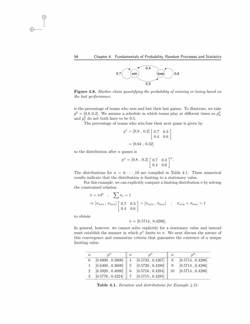
This yields the two-state markov chain illustrated in Figure 4.8 where

S = {win, lose}.

The resulting transition matrix is

P =

0.7 0.30.4 0.6

�

.

There are 30 teams in major league baseball so

p0 = [p0w , p0` ] , p0w + p0` = 1


ii

i

ii

ii


0.7 win lose

0.4

0.3

0.6

Figure 4.8. Markov chain quantifying the probability of winning or losing based onthe last performance.

is the percentage of teams who won and lost their last games. To illustrate, we takep0 = [0.8, 0.2]. We assume a schedule in which teams play at di↵erent times so p0wand p0` do not both have to be 0.5.

The percentage of teams who win/lose their next game is given by

p1 = [0.8 , 0.2]

0.7 0.30.4 0.6

�

= [0.64 , 0.32]

so the distribution after n games is

pn = [0.8 , 0.2]

0.7 0.30.4 0.6

�n.

The distributions for n = 0, · · · , 10 are compiled in Table 4.1. These numericalresults indicate that the distribution is limiting to a stationary value.

For this example, we can explicitly compute a limiting distribution ⇡ by solvingthe constrained relation

⇡ = ⇡P ,X

⇡i = 1

) [⇡win , ⇡lose]

0.7 0.30.4 0.6

�

= [⇡win , ⇡lose] , ⇡win + ⇡lose = 1

to obtain⇡ = [0.5714 , 0.4286].

In general, however, we cannot solve explicitly for a stationary value and insteadmust establish the manner in which pn limits to ⇡. We next discuss the nature ofthis convergence and summarize criteria that guarantee the existence of a uniquelimiting value.

n pn n pn n pn

0 [0.8000 , 0.2000] 4 [0.5733 , 0.4267] 8 [0.5714 , 0.4286]1 [0.6400 , 0.3600] 5 [0.5720 , 0.4280] 9 [0.5714 , 0.4286]2 [0.5920 , 0.4080] 6 [0.5716 , 0.4284] 10 [0.5714 , 0.4286]3 [0.5776 , 0.4224] 7 [0.5715 , 0.4285]

Table 4.1. Iteration and distributions for Example 4.51.


ii

i

ii

ii


As detailed in Section 4.4, it does not make sense to directly consider limitslimn!1

Xn of random variables. Instead, we consider the limit

limn!1

pn = ⇡

which is convergence in distribution. We note that if this limit exists, it must satisfy

⇡ = limn!1

p0Pn = limn!1

p0Pn+1 =⇣

limn!1

p0Pn⌘

P = ⇡P.

Definition 4.52 (Stationary Distribution). For a Markov chain with transitionkernel P , distributions ⇡ that satisfy

⇡ = ⇡P (4.38)

are termed equilibrium or stationary distributions of the chain. In a measure theo-retic framework, ⇡ is an invariant measure.

For every finite Markov chain, there exists at least one stationary distribu-tion. However, it may not be unique and it may not be equal to lim

n!1pn. Criteria

necessary to establish a unique limiting distribution ⇡ = limn!1

pn are motivated by

the following definitions and examples.

Definition 4.53 (Irreducible Markov Chain). A Markov chain is irreducible ifany state xj can be reached from any other state xi in a finite number of steps; that

is p(m)

ij > 0 for all states in finite m. Otherwise it is reducible.

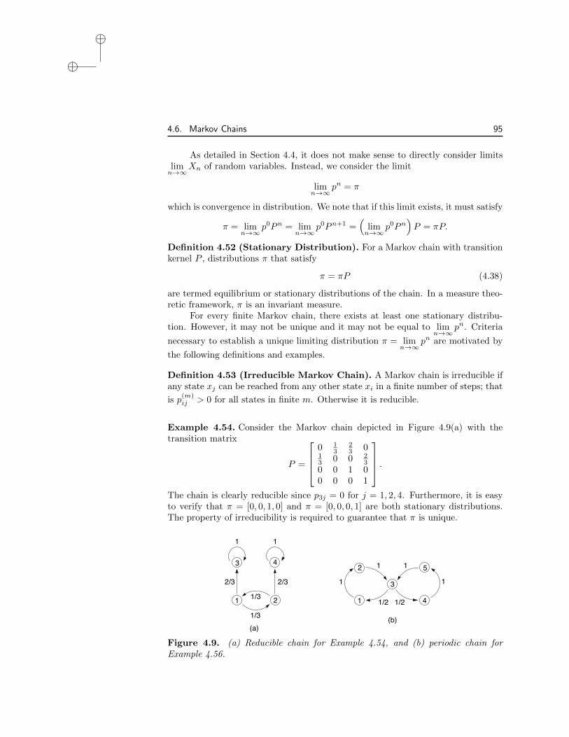
Example 4.54. Consider the Markov chain depicted in Figure 4.9(a) with thetransition matrix

P =

2

6

6

4

0 1

3

2

3

01

3

0 0 2

3

0 0 1 00 0 0 1

3

7

7

5

.

The chain is clearly reducible since p3j = 0 for j = 1, 2, 4. Furthermore, it is easy

to verify that ⇡ = [0, 0, 1, 0] and ⇡ = [0, 0, 0, 1] are both stationary distributions.The property of irreducibility is required to guarantee that ⇡ is unique.

(a)

1 21/3

1/3

1

2

3

(b)

11

5

41/2 1/2

113 4

2/3 2/3

1 1

Figure 4.9. (a) Reducible chain for Example 4.54, and (b) periodic chain forExample 4.56.


ii

i

ii

ii


Definition 4.55 (Periodic Markov Chain). A Markov chain is periodic if partsof the state space are visited at regular intervals. The period k is defined as

k = gcdn

m|⇡(m)

ii > 0o

= gcd {m|P (Xn+m = xi|Xn = xi) > 0} .

The chain is aperiodic if k = 1.

Example 4.56. The Markov chain depicted in Figure 4.9(b) with the transitionmatrix

P =

2

6

6

6

6

4

0 1 0 0 00 0 1 0 01

2

0 0 1

2

00 0 0 0 10 0 1 0 0

3

7

7

7

7

5

has the unique stationary distribution ⇡ = [1/6 , 1/6 , 1/3 , 1/6 , 1/6]. It is estab-lished in Exercise 4.8 that if p0 = [1, 0, 0, 0, 0, 0], then p3 = p6 = p9 = · · · = p0 sothe period is k = 3. Because mass cycles through the chain at a regular interval,it does not converge so lim

n!1pn does not exist. Furthermore, it is demonstrated

in Exercise 4.9 that if the limit of a periodic chain exists for one initial distribu-tion, other distributions can yield di↵erent limits. Hence aperiodicity is required toguarantee that the limit exists.

For infinite chains, one must additionally include conditions regarding thepersistence or recurrence of states. However, we will focus on finite Markov chainsfor which it can be shown that if the chain is irreducible, all states are positivepersistent [119].

Before providing a theorem that establishes the convergence limn!1 pn = ⇡,we summarize relevant results from matrix theory.

Definition 4.57. A k ⇥ k matrix A is

(i) nonnegative, denoted A � 0, if aij � 0 for all i, j

(ii) strictly positive, denoted A > 0, if aij > 0 for all i, j.

Theorem 4.58 (Perron–Frobenius). Let A be an k⇥k nonnegative matrix suchthat Am > 0 for some m � M . Then

(i) A has a positive eigenvalue �0

with corresponding left eigenvector x0

where theentries of x

0

are positive,

(ii) If � 6= �0

is any other eigenvalue of A, then |�| < �0

,

(iii) �0

has geometric and algebraic multiplicity 1.

There are several statements of the Perron-Frobenius theorem, and details andproofs can be found in [119,128,217].


ii

i

ii

ii


Theorem 4.59. For all finite stochastic matrices P , the largest eigenvalue is �0

= 1.

See [119] for a proof of this theorem.

Theorem 4.60. Let P be a finite transition matrix for an irreducible aperiodicMarkov chain. Then there exists M � 1 such that Pm > 0 for all m � M .

Further details are provided in [119] and the theorem is illustrated in Exercise 4.10.The following theorem establishes the convergence of the Markov chain.

Theorem 4.61. Every finite, homogeneous Markov chain that is irreducible andaperiodic, with transition matrix P , has a unique stationary distribution ⇡. More-over, chains converge in the sense of distributions, limn!1 pn = ⇡, for every initialdistribution p0.

Proof. It follows from Theorems 4.58–4.60 that the largest eigenvalue of P is�0

= 1 which has multiplicity 1. There is thus a unique left eigenvector ⇡ thatsatisfies ⇡P = ⇡ and

P

⇡i = 1. To establish the convergence, we first consider theeigendecomposition

UPV = ⇤ =

2

6

6

4

1 0 · · · 00 �

2

.... . .

...0 · · · �k

3

7

7

5

where 1 > |�2

| � · · · � |�k| and V = U�1. It follows that

limn!1

Pn = limn!1

V

2

6

6

4

1 0 · · · 00 �n

2

.... . .

...0 · · · �n

k

3

7

7

5

U = V

2

6

6

4

1 0 · · · 00 0...

. . ....

0 · · · 0

3

7

7

5

U.

Furthermore, we observe that UP = ⇤U implies that

2

4

⇡1

· · · ⇡k

......

uk1 · · · ukk

3

5

"

P

#

=

2

6

6

4

1�2

. . .�n

3

7

7

5

2

4

⇡1

· · · ⇡k

......

uk1 · · · ukk

3

5

and V = U�1 implies that

UV =

2

4

⇡1

· · · ⇡k

......

uk1 · · · ukk

3

5

2

4

1 · · · v1k

......

1 · · · vkk

3

5 =

2

4

1 · · · 0...

...0 · · · 1

3

5


ii

i

ii

ii


sinceP

⇡i = 1. This establishes that the first column of V is all ones. Finally

limn!1

pn = limn!1

p0Pn

= limn!1

⇥

p01

, · · · , p0k⇤

2

4

1 · · · vk1...

...1 · · · vkk

3

5

2

6

6

4

1�2

. . .�k

3

7

7

5

2

4

⇡1

· · · ⇡k

......

uk1 · · · ukk

3

5

=⇥

p01

· · · p0k⇤

2

4

1 · · · vk1...

...1 · · · vkk

3

5

2

6

6

4

10

. . .0

3

7

7

5

2

4

⇡1

· · · ⇡k

......

uk1 · · · ukk

3

5

= [⇡1

, · · · , ⇡k]

= ⇡

thus establishing the required convergence.

Theorem 4.61 establishes that finite Markov chains which are irreducible andaperiodic will converge to a stationary distribution ⇡. However, it is often di�cultor impossible to solve for ⇡ using the relations ⇡P = ⇡ subject to

P

⇡i = 1.The detailed balance condition provides an alternative that is straight-forward toimplement in MCMC methods where the goal is to construct Markov chains whosestationary distribution ⇡ is the posterior distribution for parameters.

Definition 4.62 (Detailed Balance). A chain with transition matrix P = [pij ]and distribution ⇡ = [⇡

1

, · · · , ⇡k] is reversible if the detailed balance condition

⇡ipij = ⇡jpji (4.39)

is satisfied for all i, j. Since

X

i

⇡ipij =X

i

⇡jpji = ⇡j

X

j

pji = ⇡j ,

it follows immediately that ⇡P = ⇡ so that reversibility implies stationarity. Henceif the chains are irreducible and aperiodic, they will uniquely limit to this specifiedstationary distribution. In Chapter 8, we use the Metropolis algorithm to constructchains that satisfy (4.39) and converge to the posterior density.

4.7 Random Versus Stochastic Di↵erential EquationsWe briefly illustrate here the di↵erence between random di↵erential equations, whichwe consider throughout this text, and stochastic di↵erential equations. This is donein part to allay a growing trend in the UQ community to treat these terms assynonymous when in fact they are distinctly di↵erent and they require completelydi↵erent techniques for analysis and approximation.


ii

i

ii

ii

4.7. Random Versus Stochastic Di↵erential Equations 99

Definition 4.63 (Random Di↵erential Equation). Random di↵erential equa-tions are those in which random e↵ects are manifested in parameters, initial orboundary conditions, or forcing conditions that are regular (e.g., continuous) withrespect to time and space. An example is the ODE

dz

dt= a(!)z + b(t, !)

z(0) = z0

(!)

which has the solution

z(t; q) = ea(!)t

z0

(!) +

Z t

0

e�a(!)sb(s, !))ds

�

.

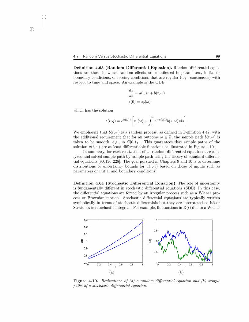
We emphasize that b(t, !) is a random process, as defined in Definition 4.42, withthe additional requirement that for an outcome ! 2 ⌦, the sample path b(t, !) istaken to be smooth; e.g., in C[0, tf ]. This guarantees that sample paths of thesolution u(t, !) are at least di↵erentiable functions as illustrated in Figure 4.10.

In summary, for each realization of !, random di↵erential equations are ana-lyzed and solved sample path by sample path using the theory of standard di↵eren-tial equations [90,136,228]. The goal pursued in Chapters 9 and 10 is to determinedistributions or uncertainty bounds for u(t, !) based on those of inputs such asparameters or initial and boundary conditions.

Definition 4.64 (Stochastic Di↵erential Equation). The role of uncertaintyis fundamentally di↵erent in stochastic di↵erential equations (SDE). In this case,the di↵erential equations are forced by an irregular process such as a Wiener pro-cess or Brownian motion. Stochastic di↵erential equations are typically writtensymbolically in terms of stochastic di↵erentials but they are interpreted as Ito orStratonovich stochastic integrals. For example, fluctuations in Z(t) due to a Wiener

0 0.2 0.4 0.6 0.8 10.7

0.8

0.9

1

1.1

1.2

1.3

t

z(t)

0 0.2 0.4 0.6 0.8 1!1

!0.5

0

0.5

1

t

Z(t)

(a) (b)

Figure 4.10. Realizations of (a) a random di↵erential equation and (b) samplepaths of a stochastic di↵erential equation.


ii

i

ii

ii


process W could be formulated as

dZ(t) = �aZ(t)dt + bdW (t)

which is interpreted as

Z(t) = Z0

�Z t

0

aZ(s)ds +

Z t

0

bdW (s)

where the second integral is an Ito stochastic integral.As illustrated in Figure 4.10, the solutions of SDE exhibit nondi↵erentiable

sample paths due to the irregularity of the driving Wiener process. We do notfurther consider SDE in this text but rather include this definition to delineatethem from random di↵erential equations. The reader is referred to [90, 136] forfurther details about SDE.

4.8 Statistical InferenceThe goal in statistical inference is to deduce the structure of, or make conclusionsabout, a phenomenon based on observed data. This often involves the determinationof an unknown distribution based on observed data in which case the problem ofstatistical inference can be stated as follows. Given a set

S = {x1

, · · · , xn} , xj 2 RN

of observed realizations of a random variable X, we want to infer the underlyingprobability distribution that produces the data S.

Statistical inference can be roughly categorized as being parametric or non-parametric in nature. In parametric approaches, one assumes that the underlyingdistributions can be adequately described in terms of a parametric relation havinga relatively small number of parameters; e.g., mean and variance. The inferenceproblem is to estimate those parameters or the distribution of those parameters.This approach has the advantage of a typically small number of parameters butthe disadvantage of limited accuracy if the assumed functional relation is incor-rect. In nonparametric approaches, one does not presuppose a functional form butinstead describes or constructs the distribution based solely on properties of theobservations. This avoids errors associated with incorrect parametric relations butrequires that some structure be imposed on algorithms to ensure that reasonabledistributions are determined.

4.8.1 Frequentist Versus Bayesian Inference

Frequentist and Bayesian inference di↵er in the underlying assumptions made re-garding the nature of probabilities, models, parameters, and confidence intervals.As detailed in [30], each approach, or a hybrid combination of the two, is advan-tageous for certain problems or applications. Hence it is necessary that scientistsunderstand both.


ii

i

ii

ii

4.8. Statistical Inference 101

From a frequentist perspective, probabilities are defined as the frequencieswith which an event occurs if the experiment is repeated a large number of times.Hence they are objective and are not updated as data is acquired. Parameters areconsidered to be unknown but fixed; hence they are deterministic. To statisticallyestablish confidence in the estimation process, one constructs estimators, such asordinary least squares (OLS) or maximum likelihood estimators (MLE), to esti-mate the parameters in the manner detailed in Section 4.3. Based on either theassumption of normality for the errors or asymptotic theory resulting from the Cen-tral Limit Theorem, one can then construct sampling distributions and confidenceintervals for the parameter estimators.

The interpretation of confidence intervals in the framework of frequentist infer-ence is often a source of confusion. As detailed in Definition 4.31, a 90% confidenceinterval has the following interpretation: in repeated procedures, 90% of realizedintervals would include the true parameter q

0

. In model calibration, this means thatif the estimation procedure is repeated 100 times using data having the same errorstatistics, and a 90% interval estimate is computed each time, then 90% of the in-tervals would include q

0

as illustrated in Figure 4.11(a). The sampling distributionand confidence intervals thus quantify the accuracy and variability of the estimationprocedure rather than providing a density for the parameter. Hence they do notprovide a direct measure of parameter uncertainty.

Because parameters are fixed, but unknown, values in this framework, itcannot be directly applied to obtain parameter densities that can be propagatedthrough models to quantify model uncertainty. In some problems, the samplingdistributions may be similar to parameter distributions but this needs to be verifiedeither experimentally or using Bayesian analysis. This is discussed in more detailin Chapter 7.

Probabilities are treated as possibly subjective in the Bayesian framework andthey can be updated to reflect new information. Moreover, they are considered tobe a distribution rather than a single frequency value. Similarly, parameters areconsidered to be random variables with associated densities and the solution of theparameter estimation problem is the posterior probability density. The Bayesianperspective is thus natural for model uncertainty quantification since it providesdensities that can be propagated through models. The interpretation of intervalestimates, termed credible intervals, is also natural in the Bayesian framework.

90% chance region q0

(a) (b)

Confidence Interval

contains value

Figure 4.11. Interpretation of a (a) frequentist 90% confidence interval and (b)Bayesian 90% credible interval.


ii

i

ii

ii


Definition 4.65 (Credible Interval). The (1�↵)⇥100% credible interval is thatwhich has a (1 � ↵) ⇥ 100% chance of containing the expected parameter. A 90%credible interval is illustrated in Figure 4.11(b).

We next provide details regarding Bayesian inference to provide the back-ground necessary for Chapter 8.

4.8.2 Bayesian Inference

Bayesian inference is based on the supposition that probabilities, and more generallyour state of knowledge regarding an observed phenomenon, can be updated asadditional information is obtained. In the context of parametric models, parametersare treated as random variables having associated densities.

Because probabilities and parameter densities are conditioned on observations,Bayes’ formula

P (A|B) =P (B|A)P (A)

P (B)

for probabilities provides a natural genesis for Bayesian inference. In the contextof parameters Q = [Q

1

, · · · , Qp] that are quantified based on observations � =[�

1

, · · · , �n], one employs the relation

⇡(q|�) =⇡(�|q)⇡

0

(q)

⇡⌥

(�)(4.40)

where ⇡0

(q) and ⇡(q|�) respectively denote the prior and posterior densities, ⇡(�|q)is a likelihood, and the marginal density ⇡

⌥

(�) is a normalization factor. Hereq = Q(!) denotes realizations of Q. We note that the subscripts which indicatespecific random variables are typically dropped from the prior and posterior inBayesian analysis.

The prior density ⇡0

(q) quantifies any prior knowledge that may be knownabout the parameter before data is taken into account. For example, one mighthave prior information based on similar previous models, data that is similar toprevious data, or initial parameter densities that have been determined throughother means such as related experiments.

For most model calibration, however, one does not have such prior informationso one uses instead what is termed a noninformative prior. A common choice ofnoninformative prior is the uniform density, or unnormalized uniform, posed on theparameter support. For example, one might employ

⇡0

(q) = �[0,1)

(q),

for a positive parameter. This choice is improper in the sense that the integral of⇡0

(q) is unbounded. It is recommended that a noninformative prior be used unlessgood previous information is known since it is shown in Example 4.66 that incorrectprior information can degrade (4.40) far more than a noninformative prior.

In “empirical Bayes” inference, one also encounters data-dependent priors inwhich priors estimated using frequentist techniques such as maximum likelihood are


ii

i

ii

ii


employed in the Bayesian model. It is argued in [35] that this double use of datais problematic with small sample sizes and is at odds with the tenets of Bayesiananalysis.

The term ⇡(�|q), which is a function of q with � fixed, quantifies the likelihoodL(q|�) of observing � given parameter realizations q as detailed in Section 4.3.2.We will illustrate various choices for the likelihood function in the examples at theend of this section and at the beginning of Chapter 8. The joint density is given by

⇡(q, �) = ⇡(�|q)⇡0

(q)

and is normalized to unity by the marginal density function ⇡⌥

(�) of all possibleobservations.

Finally, the posterior density ⇡(q|�) quantifies the probability of obtainingparameters q given observations �. It is the posterior density that we will beestimating using the Bayesian parameter estimation techniques of Chapter 8 and wepoint out that the data directly informs the posterior only through the likelihood.Finally, representation of ⇡

⌥

(�) as the integral over all possible joint densities yieldsthe Bayes relation

⇡(q|�) =⇡(�|q)⇡

0

(q)R

Rp ⇡(�|q)⇡0

(q)dq(4.41)

commonly employed for model calibration and data assimilation.A significant issue, which will be discussed in detail in Chapter 8, concerns

the evaluation of the normalizing integral. It can be analytically evaluated only inspecial cases and classical tensored quadrature techniques are e↵ective only in lowdimensions; e.g., p 4. This has spawned significant research on high dimensionalquadrature techniques including adaptive sparse grids for moderate dimensionalityand Monte Carlo techniques for high dimensions; see Chapter 11.

Example 4.66. To illustrate (4.41) in a setting where the posterior density canbe computed explicitly, we consider the results from tossing a possibly biased coin.The random variable

⌥i(!) =

⇢

0 , ! = T1 , ! = H

represents the result from the ith toss and the parameter q is the probability ofgetting heads. We now consider the probability of obtaining N

1

heads and N0

tailsin a series of N = N

0

+ N1

flips of the coin.Because coin flips are independent events with only two possible outcomes,

the likelihood of observing a sequence � = [�1

, · · · , �N ], given the probability q, is

⇡(�|q) =NY

i=1

q�i(1 � q)1��i

= qP

�i(1 � q)N�P

�i

= qN1(1 � q)N0


ii

i

ii

ii


which is simply a scaled binomial density. We consider first a noninformative prior

⇡0

(q) =

⇢

1 , 0 q 10 , else

which yields the posterior density

⇡(q|�) =qN1(1 � q)N0

R

1

0

qN1(1 � q)N0dq=

(N + 1)!

N0

!N1

!qN1(1 � q)N0 .

We note that in this special case, the denominator is the integral of a beta functionwhich admits an analytic solution. In general, however, quadrature techniques mustbe employed to approximate the integral.

For a fair coin with q0

= 1

2

, the posterior densities associated with variousrealizations N

1

and N0

are plotted in Figure 4.12. It is first observed that Bayesianinference yields a posterior density with just one experiment whereas frequentistanalysis would specify a probability of either 0 or 1. It is also observed that thevariability of ⇡(q|�) decreases as N increases. Finally, the manner in which the datainforms the density is illustrated by comparing the results with 5 Heads, 9 Tails,which has a mode of 0.36, to those of 49 Heads, 51 tails which has a mode of 0.495.This illustrates that the method is achieving the goal of having the data informwhen there is no prior information.

We next illustrate the e↵ect of a poor choice for the prior density. For thesame fair coin (q

0

= 1

2

), we consider the choice

⇡0

(q) =1

�p

2⇡e�(q�µ)2/2�2

with µ = 0.3 and � = 0.1. We cannot analytically evaluate the denominator in thiscase so we instead employ Gaussian quadrature. As illustrated in Figure 4.13, evenfor a realization of 50 Heads and 50 Tails, the mean of the posterior is still smallerthan q

0

= 1

2

but is significantly better than the result for 5 Heads and 5 Tails. Thisillustrates the manner in which a poor informative prior can have negative impactfor a large number of observations. Hence if the validity of an informative prior isin doubt, it is recommended that a noninformative prior be used instead.

0 0.2 0.4 0.6 0.8 10

0.5

1

1.5

2

1 Head, 0 Tails

0 0.2 0.4 0.6 0.8 10

1

2

3

4

5 Heads, 9 Tails

0 0.2 0.4 0.6 0.8 10

2

4

6

8

10

49 Heads, 51 Tails

Figure 4.12. Posterior densities associated with a noninformative prior for threerealizations of the coin toss experiment.


ii

i

ii

ii


0 0.2 0.4 0.6 0.8 10

1

2

3

4

5

5 Heads, 5 Tails

0 0.2 0.4 0.6 0.8 10

2

4

6

8

10

50 Heads, 50 Tails

Figure 4.13. Posterior densities associated with a poor informative prior for tworealizations of the coin toss experiment.

Conjugate Priors

Definition 4.67 (Conjugacy). The property that the prior and posterior distri-butions have the same parametric form is termed conjugacy. When this occurs, theprior ⇡

0

(q) is termed a conjugate prior for the likelihood ⇡(�|q). Parameters in theprior relation are often termed prior hyperparameters to distinguish them from themodel parameters q. The corresponding parameters in the posterior relation arecalled posterior hyperparameters.

The use of conjugate priors, when possible, is advantageous since closed formexpressions for the posterior are then available. This will be used when estimatingdensities for measurement errors in Chapter 8.

Example 4.68. Consider the binomial model

⇡(�|q) = qN1(1 � q)N�N1 , N1

=NX

i=1

�i

used for the likelihood in the coin toss Example 4.66. We observe that if the prior isparameterized similarly, the product of the prior and likelihood will be in the samefamily. Specifically, we take ⇡

0

(q) to be a beta density with hyperparameters ↵ and� so that ⇡

0

(q) / q↵�1(1 � q)��1 as shown in Definition 4.16. It then follows thatthe posterior density satisfies

⇡(q|�) / qN1(1 � q)N�N1q↵�1(1 � q)��1

= qN1+↵�1(1 � q)N�N1+��1

so it is a beta density with shape parameters N1

+ ↵ and N � N1

+ �. The betaprior distribution is thus a conjugate family for the binomial likelihood.

Example 4.69. Here we consider normally distributed random variables with knownmean µ and unknown variance �2. This will illustrate techniques employed in Chap-ter 8 to estimate the unknown variance �2

0

of measurement errors. As detailed inSection 4.3.2, the likelihood of observing � = [�

1

, · · · , �N ] iid measurements under


ii

i

ii

ii


these assumptions is

⇡(�|�2) =1

(2⇡�2)n/2e�SS/2�2

where the sum of squares error is

SS =nX

j=1

(�j � µ)2.

This likelihood is in the inverse-gamma family, defined in Definition 4.14, so theconjugate prior is ⇡

0

(�2) / (�2)�(↵+1)e�/�2

. The posterior density can then beexpressed as

⇡(�2|�) / ⇡0

(�2)⇡(�|�2)

/ (�2)�(↵+1)e��/�2

(�2)�n/2e�SS/2�2

= (�2)�(↵+1+n/2)e�(�+SS/2)/�2

so that�2|� ⇠ Inv-gamma(↵ + n/2, � + SS/2).

As shown in Definitions 4.13 and 4.14, if X ⇠ Gamma(↵, �), then Y = X�1 ⇠Inv-gamma(↵, �). This equivalence can be exploited so that the MATLAB com-mand gamrnd.m can be used to generate random numbers from a gamma distribu-tion which can then be used to construct random values from an inverse-gammadistribution.

4.9 Notes and ReferencesThis chapter provides an overview of statistical topics that play a role in uncertaintyquantification and we necessarily leave details to the following references. Thetext [60] provides a very accessible introduction to probability, point and intervalestimation, hypothesis testing, analysis of variance and linear regression with clearlystated definitions. The texts [110, 168] are also excellent sources for obtaining anoverview of probability and statistics at an upper undergraduate level. The book[95] delineates the di↵erence between estimators and estimates by using di↵erentnotation and is an excellent source for details regarding linear regression. Finally,[80, 81] are classics in the field of probability.

There are a number of excellent supplemental texts on random processes andMorkov chains including [98, 119, 124, 128, 156, 181, 251]. Additional theory, exam-ples, and numerical algorithms for random and stochastic di↵erential equations canbe found in [90, 136, 183, 228]. We note that due to the mathematical nature ofthe underlying framework required for stochastic di↵erential equations, these lattertexts also provide a measure-theoretic framework for random variables and otherconcepts discussed in this chapter. Additional details regarding a measure theoreticbasis for aspects of this material can be found in [36].

The reader is referred to [56, 221] for introductory concepts and examples re-garding Bayesian analysis and computing and [34,91] for a more in-depth treatment

chapter 4 fundamentals of probability, random processes ... · fundamentals of probability, random...

Documents