317

CHAPTER 4

FORECASTING THE VALUES OF EXOGENOUS VARIABLES:

TRANSPORTATION SYSTEM ATTRIBUTES

Introduction

The development and use of disaggregate travel demand models fortransportation policy analyses requires auxiliary forecasts of the variablesexogenous to the model system. The previous chapter described a method ofdeveloping the exogenous socioeconomic attributes for a homogenous marketsegment or for a representative sample of households. In this chapter a method isdescribed that provides estimates for the various components of travel time on thevarious modes of travel as a function of the transportation system serving adoor-to-door trip from a given origin zone to a known destination zone. The samemethod can be used to forecast those items of trip user costs that are definedfunctions of trip distance.

The two measures, travel time and travel costs and their components, areoften used to completely characterize the performance of the transportation systemin travel demand models. This is not to say that such measures as on-timeperformance, security, safety, and other system attributes are not important, butthat current knowledge of them is limited. It is acknowledged, then, that moreresearch is needed to quantify those variables but the matter is not pursued here. Another point to note is that headways of buses are taken to be exogenousvariables; the feedback of demand through management is assumed not to exist.

318

The use of networks to compute the travel times and costs is so ingrainedamong transport planners that the use of anything else to represent transportsystem performance is considered to be a questionable shortcut or viewed as a"back-of-the-envelope" computation. Nonetheless, the use of networks hasseveral disadvantages and shortcomings (Talvitie and Dehghani, 1976; see alsoPart IV, Chapter 8) that encourage the development of alternative methods tocomputing network independent "supply" models. These are the accuracy ofnetwork calculations in computing trip times and the aggregation of individualdemands to obtain total demand. As noted by Talvitie (1973), McFadden andReid (1975), and Westin (1975), unbiased aggregation of individual traveldemands requires that the within-group variances are accounted for. However, thenetworks provide only one estimate of level-of-service per mode for an O-D pair;that is, the within-zone variance of level-of-service attributes is assumed to bezero. Is this a reasonable assumption, or more generally do the minimum pathalgorithms operating within coded networks provide accurate values forlevel-of-service to be used either in developing the travel demand models or inforecasting with them? An examination of this issue is undertaken in the next twosections of this chapter.

In the third and fourth sections a method and models are developed anddescribed which permit network-independent description of travel time on variousmodes for access and linehaul. These models are used in a transport corridorpolicy study (FRX).

1This does not guarantee that the chosen or �would be chosen� path was actually measured. A check waspossible with those who reported which path they took (occasional and regular transit users) against what wasmeasured. These paths agreed in seventy-six of the eighty-six cases where the information was available. Ofthe ten misses, five persons took a different bus route altogether, in the other five misses one part of the busroute was different. Thus, there is some justification to take issue with the use of the word �experienced� inthis paper. Those of the readers who prefer to do so should regard this paper as a comparison of twodifferent algorithms to choose a transit path and hence the travel time components of a door-to-door trip.

319

A Comparison of Experienced and Network Based Travel Time Measurements

To start, we need to define the way in which the two types of values wereobtained. The experienced transit travel times were obtained by asking the transitagencies� information service to route travelers as if an inquiry call for a transitroute were made by the traveler.1 The experienced auto travel times were basedon travel time runs (moving vehicle method) made at various times of day and byrouting travelers at the minimum time path at their time of travel.

The network values were obtained through standard network models andassociate either peak or off-peak values with the traveler depending on when thetrip took place. These data were prepared independently of the present researchand are reported in McFadden (1973b). (For a detailed account of the datapreparation see articles by M. Johnson and F. Reid in that publication.) Roundtrip travel time and cost values are used in both sets of data. The comparison ofthe types of measurements will be done in two different ways by comparing themeasurements directly using various indices and by comparing the modelsestimated with the two types of measurements.

Means, standard deviations, and correlation coefficients

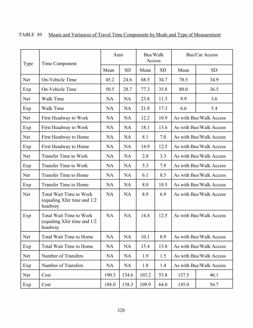
The comparison of the experienced (E) and network (N) travel times maybe started by listing the means and variances of the travel time components ofinterest. These appear in Table 49. Examination of the values in Table 49 revealsno spectacular differences; the variances in the "experienced" data cells appear tobe consistently higher and the means differ somewhat. The greatest concern, onthe basis of the values in Table 49 appears to be with the headway of the first busand with the transfer times, either to work or to home. This difference can, atleast in part, be attributed to headways that can vary substantially within peakhours.

320

TABLE 49 Means and Variances of Travel Time Components by Mode and Type of Measurement

Type Time Component

Auto Bus/WalkAccess

Bus/Car Access

Mean SD Mean SD Mean SD

Net On-Vehicle Time 45.2 24.6 68.5 34.7 70.5 34.9

Exp On-Vehicle Time 50.5 28.7 77.3 35.8 80.0 36.5

Net Walk Time NA NA 23.8 11.5 9.9 3.6

Exp Walk Time NA NA 21.8 17.3 6.6 5.4

Net First Headway to Work NA NA 12.2 10.9 As with Bus/Walk Access

Exp First Headway to Work NA NA 18.1 13.6 As with Bus/Walk Access

Net First Headway to Home NA NA 8.1 7.0 As with Bus/Walk Access

Exp First Headway to Home NA NA 14.9 12.5 As with Bus/Walk Access

Net Transfer Time to Work NA NA 2.8 3.3 As with Bus/Walk Access

Exp Transfer Time to Work NA NA 5.3 7.9 As with Bus/Walk Access

Net Transfer Time to Home NA NA 6.1 8.5 As with Bus/Walk Access

Exp Transfer Time to Home NA NA 8.0 10.5 As with Bus/Walk Access

Net Total Wait Time to Work(equaling Xfer time and 1/2headway

NA NA 8.9 6.9 As with Bus/Walk Access

Exp Total Wait Time to Work(equaling Xfer time and 1/2headway

NA NA 14.4 12.5 As with Bus/Walk Access

Net Total Wait Time to Home NA NA 10.1 8.9 As with Bus/Walk Access

Exp Total Wait Time to Home NA NA 15.4 13.8 As with Bus/Walk Access

Net Number of Transfers NA NA 1.9 1.5 As with Bus/Walk Access

Exp Number of Transfers NA NA 1.8 1.4 As with Bus/Walk Access

Net Cost 190.3 134.6 103.2 53.8 137.5 46.1

Exp Cost 188.0 138.3 109.9 64.0 145.0 56.7

1This coefficient is computed as (�

i(Ni � Ei)

2 / (�i

(N 2i � E 2

i ))1/2 .

The numerator can be decomposed into three components and normalized to unity.

321

"Total wait time," which is the sum of cumulative transfer times and one-half offirst headway, confirms that differences exist in the two types of measurement: theexperienced values being higher than the network values. In summary, exceptingthe walk time whose mean is just two minutes higher by the network algorithm,all the mean values from the network are somewhat lower than the correspondingvalues experienced by the travelers. The standard deviations of the experiencedtravel times are substantially larger than those of the network times. It may becomputed from Table 49 that between zone variance (network data) accounts forthirty to sixty percent of the total variance (experienced data) for the excess timecomponents and about seventy to ninety percent of the on-vehicle time variances. This must have a bearing on aggregation as will be discussed later.

The values of the correlation coefficients, regression intercepts, and"slopes" in Table 50 indicate that other than the on-vehicle times, the desiredvalues of unity and zero for correlation intercept and slope are not achieved; evenfor the on-vehicle times the hypothesis that the slope b equals unity must berejected.

Root mean square errors and Theil-U coefficients

The information produced so far about the similarities and dissimilaritiesof objective and network measurements of travel times can be convenientlysummarized using two measures: the root mean square error and Theil'sU-coefficient.1 The former is often used as an "all around" measure of"goodness-of-fit;" the latter measure is zero for perfect measurements (orforecasts) and has an upper bound of one. Theil's U-coefficient can furthermorebe decomposed to three components, denoted UM , US , UC , which indicate theproportional loss in accuracy that is due to differences in means, in standarddeviations, and in covariances, respectively. These useful summary measures aregiven in Table 51.

322

TABLE 50 Correlation Coefficients, Intercepts, and Slopes for RegressionsBetween Some of the Experienced and Network Times

Travel Time Component

CorrelationCoefficient

Intercept a

(std error)

Slope b

(std error)

Auto Round-Trip On-vehicle Time

.91 6.52 (1.73) .766 (.030)

Bus Round-Trip On-vehicle Time

.89 1.83 (3.18) .862 (.037)

Walk Time Bus/WalkAccess

.45 17.28 (1.40) .297 (.050)

Walk Time Bus/AutoAccess

.32 8.45 ( .45) .213 (.050)

Headway on Bus toWork

.52 4.64 (1.32) .416 (.058)

Transfer-Time on Busto Work

.35 2.07 ( .32) .144 (.033)

Headway on Bus toHome

.50 3.91 ( .79) .279 (.041)

Transfer-Time on Busto Home

.38 3.68 ( .83) .303 (.063)

323

TABLE 51 Root Mean Square Errors and Theil U-coefficients of Travel TimeComponents by Network Measurements as Compared to theExperienced Travel Times

Variable Means (experienced)

RMSE Theil U

U UM US UC

On-vehicle time - auto 50.5 13.1 .17 .16 .10 .74

On-vehicle time -bus(w)a 77.3 18.8 .16 .22 .00 .78

On-vehicle time - bus(a) 80.0 19.3 .16 .24 .01 .75

Walk time - bus(w) 21.8 16.0 .42 .02 .13 .85

Walk time - bus(a) 6.6 6.4 .47 .27 .08 .65

Headway to work 18.1 13.6 .49 .19 .04 .77

Headway to home 14.9 12.8 .58 .28 .18 .54

Transfer-time to work 5.3 7.8 .75 .10 .35 .55

Transfer-time to home 8.0 10.9 .65 .04 .03 .93

a/ w, a denote access mode - a = auto, w = walk

1The sample size was 142; there were 103 auto users, twenty-eight bus riders with walk access and elevenbus riders with car access.

324

The results in Table 51 are revealing. Excepting the linehaul travel times,the root mean square errors are roughly equal in magnitude to the means of theexperienced travel times indicating rather large errors in measurement. The sameresult is conveyed by the Theil U- coefficient. Again, the U-coefficient obtainsvery large values for out-of-vehicle time components, even for on-vehicle timecomponents the U-coefficient, (and the RMSE) is quite high. One wonders iftravel forecasts would be as highly regarded as network travel time data if theywere subject to errors of these magnitudes. Finally, the components of theU-coefficient indicate that the largest share of the error comes from thecovariances between the network and objective measurements; in some cases asubstantial part is also due either to differences in means or standard deviations.

Frequency plots of model variables

As a final item before actually estimating choice models using the twotypes of measurement, it is instructive to examine the frequency plots of some ofthe travel time variables. The analysis performed by McFadden and Reid (1975)tells that zonal averages will yield consistent estimates for coefficients given thatthe distributions of variables within a zone are not skewed. Thus, the distributionof the variables for the entire sample (envisioned as one large zone) ought not tobe skewed either if good coefficients are to result from using zonal averages. Thecomparison of frequency distributions will also help state a priori expectations forthe model coefficients; however, for two reasons caution must be exercised indoing so. First, because the logic model operates on differences, the distributionsought to be plotted separately by choice and the difference examined; due to thesmall sample size this was not possible.1 Second, the components of the TheilU-coefficient indicated that most of the difference between the two types ofmeasurements is due to covariances. This means that the frequency plots for thetwo measurements can look similar without the measurements being similarbecause measurements in any given interval may not pertain to the sameindividuals.

325

It is natural to start with the plots of auto and transit (with walk access)on-vehicle times; these are shown in Figure 13 (auto), (bus), and (bus minus auto). A visual examination of the plots in Figure 13 suggests that there is a great deal ofsimilarity between the two types of measurements; the only noticeable differenceis the "fat tail" of the experienced auto on-vehicle times distribution. One mightsuspect that the lack of "fat tail" in the network times distribution is due toimproper accounting of congestion effects. A χ2 test against the null hypothesisthat the distribution of network times is identical to the distribution of theexperienced travel times had to be rejected, however, at the .95 level ofconfidence.

The walk time (bus-with-walk-access) frequency distribution in Figure 13indicates that the network-coded walk time has a highly peaked distribution whilethe distribution of the experienced walk times both peaks earlier and is much"fatter." The appearance of the two distributions is as expected. Traffic zones areconnected to the network with relatively few common values, and the experiencedvalues show a scatter that relates to the location of individuals with respect to thebus line configuration.

The frequency plot for bus headways (round trip; directional headwayssummed) appears also in Figure 14. It may be noted that the network headwaysare shorter in duration; their distribution also has a noticeably thinner tail than thatof the experienced headways. The apparent reason is that zones have beenconnected to trunk-line streets on which many bus lines operate and have lowheadway for consecutive buses, when actually the travelers� origins anddestinations are dispersed within the zones, and by taking note of schedules, thetravelers can gain the advantage of nearer buslines in spite of their lower servicefrequency.

Finally, a look at the frequency plot for transfer time indicates that thedistributions for transfer time resemble each other; they are also the onlydistributions where the null hypotheses that network travel time distribution is thesame as the distribution of experienced travel times cannot be rejected at the .99level of confidence. It is surprising that transfer time distributions are so similar,because at least fifty-six percent of the travelers are known to take different paths;the Theil U-coefficient was also very high for the transfer times: however, most ofthe error was due to covariances that may explain the outcome.

326

327

328

In order to capture the non-linearity of travelers� response to transitheadways in modeling choice, to be reported in the next section, the headways aresegmented into two components (see also Chapters 1 and 2, Part II). The firstcomponent of the headway is up to a maximum of eight minutes, and the secondcomponent is the remaining headway time. In order to do justice to both legs of around-trip, these two components have been computed separately for bothdirections and then summed. The plots of the two headway segments appear inFigure 15. It may be noted that the distributions for the truncated portion of theheadway are quite similar (note, however, the scale on the vertical axis) while thetail sections of the headway have quite different distributions; the latter is alreadyevident from Figure 15.

Discussion

This section may be concluded by noting that the two types ofmeasurements--experienced and network--of travel time variables are certainlydifferent. On the basis of the frequency plots one would expect that similarcoefficients can, nevertheless, be estimated for on-vehicle time, transfer time, andfirst component of the headway regardless which type of measurement is used. However, one must keep in mind that for these variables most of the error was dueto covariances and cannot be seen in the plots; thus, if the experienced traveltimes are strongly correlated with socioeconomic variables or with each other,then the anticipation of similar coefficients will fail. This latter is most certainlytrue with the headway variable; the first component must correlate highly with thesecond component because well over one-half of the travelers had round-tripheadways greater than sixteen minutes. Correlations between socioeconomic andtravel time variables will also exist: transportation folklore suggests that bus walktimes and socioeconomic variables are highly correlated. Finally, it may be notedthat the experienced travel times have distinctly skewed distributions; this, it maybe recalled, violates one of the conditions for obtaining consistent coefficientestimates using zonal averages measured by the network models. The comparisonof mode choice models using the two types of supply variable measurementsfollows next.

329

1For specification of the variables and the coefficients of the McFadden, Train model, see Table 2, Part II,Chapter 1.

330

A Comparison of Mode Choice Models Developed with Two Types of SupplyMeasurements

The "basic model" specifications used as a benchmark here is the onereported by McFadden and Train (1975).1 Table 52 shows the coefficients for thatmodel (labeled Model Ax; x = N for network or x = E for experienced) andanother model, labeled B , whose specification includes the second, untruncatedportion of the headway and no transfer time, which was deleted from the B model due to the coefficient instability and closeness to zero. The two models areestimated using both experienced and network travel time measurements.

The discussion of these models will be focused on the transportationsystem performance variables: travel times and travel costs. The socioeconomicvariables, which are common to both (N and E) type models and pertain toindividuals rather than zones, are discussed only insofar as their deletion orinclusion affects the coefficients for the travel time or cost components.

A number of points are worth noting in comparing the xN and xE typemodels. First, the coefficient for travel cost is stable across the models, regardlessof the type of measurement. Second, the on-vehicle travel time coefficient istwice as high in the models estimated with experienced travel times as comparedto the model estimated with network travel time measurements. On the otherhand, the coefficient for walk time behaves exactly in the opposite way. It is as ifthese two variables have exchanged coefficients in the two types of models; andthere is no reporting error here. The values of time computed from these modelsare, naturally, similarly reversed. In the E series models the value of theon-vehicle time is around seventy percent of the wage rate and the value of walktime nearly forty percent of the wage rate. In the N series models these twofigures are around forty and eighty-five percent, respectively. The behavior of thetraveling time coefficients, especially that of walk time, is such that one is led tosuspect the underlying correlations to be secretly at work. For example, from thedistribution of the walk times in Figure 14 one is willing to surmise that thecoefficient of experienced walk times will be higher than the one estimated fornetwork measured walk time. This is because the distribution of experiencedwalk times is located to the left of the distribution of network walk times. Morewill be said about walk times later.

331

TABLE 52 Coefficients (t-values) of Work Trip Mode Choice Models Estimated Using Both Experienced andNetwork Travel Times

Model AEExperienced TravelTimes

Model AN NetworkTravel Times

Model BEExperienced TravelTimes

Model BN NetworkTravel Times

INC 1 .000413 (1.4) .000239 ( .80) .000339 (1.1) .000279 ( .90)

INC 2 .000955 (1.8) .000684 (1.4) .0001075 (1.9) .000592 (1.2)

INC 3 -.000743 (2.6) -.000643 (2.5) -.000748 (2.6) -.000624 (2.4)

Residence .178 . (3.0) .193 (2.9) .176 (3.0) .195 (3.0)

Population Density -.643 (2.1) -.449 (1.5) -.713 (2.1) -.480 (1.6)

Parking -.433 (1.2) -.308 ( .92) -.384 (1.0) -.316 ( .90)

Age -.759 (1.1) -.711 (1.02) -.720 (1.0) -.735 (1.1)

Child -1.575 (2.3) -.969 (1.50) -1.676 (2.4) -1.049 (1.6)

Drivers 1.321 (2.8) 1.182 (2.7) 1.248 (2.6) 1.186 (2.7)

Cost/Wage -.0427 (3.1) -.0468 (3.1) -.0448 (3.1) -.0473 (3.1)

On Time -.0293 (1.8) -.0132 ( .60) -.0304 (1.9) -.0175 ( .90)

Walk Time -.0157 ( .74) -.0418 (1.3) -.0185 ( .90) -.0379 (1.1)

Transfer-Time -.0395 (1.0) -.0346 ( .80) --- ---

Number of Transfers -.165 ( .50) -.0387 ( .20) -.321 (1.3) -.134 ( .6)

Headway 1 (< 8 min) -.242 (2.1) -.246 (2.3) -.137 (1.1) -.216 (2.4)

Headway 2 (> 8 min) ------ --- -.0647 (1.9) -.0427 (1.8)

Da -6.399 (2.3) -4.806 (1.9) -5.159 (1.9) -4.640 (1.8)

Dba -2.806 (3.2) -2.989 (3.4) -2.724 (3.1) -2.932 (3.3)

Likelihood ratio index .601 .575 .613 .578

% Right 81.7 83.1 82.4 84.5

Value of On-Time 69% of wage 28% of wage 68% of wage 37% of wage

Value of Walk Time 37% of wage 89% of wage 41% of wage 80% of wage

Ratio of Walk/On-Time .54 3.17 .61 2.17

332

The third outstanding item in Table 52 has to do with the coefficients forthe number of transfers, headways, and transfer time. The number of transfers hasabout a three times higher coefficient in the models using experienced routeinformation; the two headway components also have different weights in the twotypes of models. If only the truncated portion of the headway is included in themodel--as was done in Models AE and AN--then this headway coefficient in thetwo types of models has just about the same value. This is an interesting outcome(it can be surmised by looking at the frequency distributions of these variables inFigure 15) and will be discussed later. Model estimations also showed that thecoefficient for transfer time became very unstable and close to zero when the tailsection of the first headway was added to the set of independent variables. Thisoutcome may be partially due to the fact that when transfers are involved, thetransfer headway is often equal to the first headway in the return trip. Thus, withtruncation of the first headway, something is the matter with transfer time;however, when the first headway is not truncated the effect of the transfer timeseems to fall off. (See also discussion in Part II, Chapter 2.)

The fourth and final item evident from Table 52 is the low statisticalsignificance of most of the coefficients and the equal forecasting accuracy of themodels, as judged from the likelihood ratio and percent right indices. Given thelow statistical significance of the system variables, one can rightly ask are themodels developed using the two different supply measurements statisticallydifferent? The answer appears to be no. This result was arrived at by performinga sort of Chow-test on the two models (McFadden, 1973). The coefficients werefirst estimated using the combined sample (284 observations) and restricting thecoefficients of two types of measurements to be equal and then relaxing thisrestriction and performing the likelihood test on the results.

The χ2 distributed test-statistic with six degrees of freedom had a value of 6.8,which is well below the .95 level critical value of 12.5. Note however thatobservations in the two subsamples are not independent, putting in question thestatistical validity of the test.

Further discussion of results

In evaluating the outcome of the statistical test conducted above it is goodto keep in mind that the sample size used here was quite small and that most ofthe system variables did not obtain statistical significance in the original modelsof Table 52 at the level used in the Chow-test test. In fact, the results of that table

1It is pertinent to remind the reader that the walk and headway times (and transfer times) were previously thevariables that "caused trouble" in validation, see Part II.

333

give grounds for pursuing the matter of network measured attributes andexperienced attributes a little further. A convenient starting point for doing this isprovided by estimating a simpler model than that in Table 52; the discussionpromised earlier regarding the walk times and headways is appropriatelyconducted here also.1

It is seldom the case that all the socioeconomic variables used in themodels applied here are available for the model development of travel forecastingin particular. A question then arises about the effect of dropping some of themfrom the models; that is, what is the effect of model misspecification on theresults. Specifically, let us assume that variables "length of residence,""population density" (as defined here), "parking index," "age," "child-dummy,"and "the number of drivers" are unavailable for model estimation; and let us alsoeliminate the number of transfers from the model and truncate the headway (toform a wait time); these are all quite reasonable assumptions and customarilymade. The models estimated with the remaining variables using the two types ofsupply measurements appear in Table 53. The results show that, excepting thetransfer time, all the coefficients bear statistical significance at reasonable levelsof confidence (one-tailed tests) in the model estimated using experienced traveltime information. In the network-based model, on-vehicle time and the one-income component in addition to transfer time have low statistical significance. Particular attention should generally be paid to values of time that have climbedup substantially due to a nearly fifty percent decrease in the cost coefficient and a100 percent increase in the walk time coefficient. Also of interest is the lowcoefficient (and statistical significance) of the on-vehicle time in the networkbased model; this dilemma is almost daily experienced by travel demand modelersworking with network-based LOS information. On the other hand, theexperienced on-vehicle time coefficient has not substantially changed from theresults obtained earlier.

These changes, especially in the walk time coefficient, must be attributedto their correlation with the socioeconomic variables which were eliminated fromthe model. These correlations between the socioeconomic and transportationsystem variables are related to the locational and transportation choices that

1Past data indicate that people adjust to changes in their circum stances (and vice versa)--for whateverreason--reasonably quickly. Of about 100 working travelers in 1972 only about twenty percent had the sameorigin and destination in 1975 (UTDFP panel travel survey).

334

people make under their own circumstances.1 The "experienced" LOS valuespreserve these correlations and are likely to yield unbiased coefficients anddemand elasticities (given a good model specification) while the networkcalculations do not appear to preserve these correlations, and, by simple logic,must yield biased coefficients.

The effect of the variable specification also deserves examination. Inparticular, attention is drawn to the coefficients of the headway variables. It maybe noted from Tables 52 and 53 that if only the truncated part of the headway (inthis case up to eight minutes, one way) is included in the model its coefficientremains very nearly the same, regardless of the type of measurement. It may berecalled that the frequency plots of this variable were also very similar for bothtypes of measurement. The implication is that the construction of the variable hasprocreated the nearly identical coefficients.

335

TABLE 53 Coefficients (t-values) of Purposefully Underspecified ModeChoice Models Estimated Using Both Experienced and NetworkSupply Data

Variable Experienced

SupplyData

NetworkSupplyData

INC 1 .000207 (1.5) .000154 ( .8)

INC 2 .000961 (2.1) .000693 (1.7)

INC 3 -.000046 (1.9) -.000364 (1.7)

Cost/Wage -.0237 (2.2) -.0259 (2.6)

On-vehicle Time -.0239 (1.8) -.00394 ( .2)

Walk Time -.0377 (2.0) -.0724 (2.3)

Transfer Time -.0228 (1.0) -.0408 (1.1)

Headway 1 -.257 (2.7) -.277 (4.1)

Da -5.42 (2.8) -4.84 (3.0)

Dba -1.29 (2.6) -1.82 (3.1)

Likelihood ratio index .484 .482

% Right 76.8 76.8

Value of On-time 101 15

Value of Walk Time 159 280

Value of Xfertime(as % of wage) 96 158

Ratio Walk/On-time 1.58 18.4

1The perceptive reader may ask, then why does the on-vehicle time have such a low coefficient in thenetwork-based model in Table 53? A hypothesis can again be made that if we omit most of thesocioeconomic variables, then the choice will be attributed to the system variables; however, in building thepaths using the network models such a low weight is given to the linehaul time that linehaul time really doesnot matter in choosing a path; and a result which is a statistical artifact will follow. The hypothesis in themain text is preferred, however, because it is more general and can encompass both types of situationsencountered.

336

There is good reason to take this implication a few steps further. It may beobserved from Table 52 that the relative magnitudes of on-vehicle and walk timecoefficients are between two to three for the network-based models. This is veryclose to the relative weight (two; plus penalties for waiting and a limit ontransfers) of walk time used in building the transit paths. The obvious hypothesisthen is that the conventions used in building the paths and coding the networksprocreate the choice models based on these types of supply data.1 Thus, ifnetworks in two or more cities are coded using similar conventions and withoutregard to correlations with socioeconomic variables, and if paths are built usingsimilar weights, and variables created using the same type of rules (e.g., wait timeis one half of the head way up to ten minutes of headway and one-fourththereafter; this is quite akin to the eight minute maximum used here), then with anormally low percentage of transit users the resulting choice models for thosecities should indeed be nearly identical. The models so obtained are not reallybehavioral nor transferable--in a true sense--travel demand models. They are notlikely to predict correctly travelers� behavior when service changes occur.

If the hypothesis that network-based supply measures procreate the choicemodel coefficients is true, then it logically leads to the unfortunate conclusion thatthe accumulated evidence from numerous studies on travel demand elasticitieswith respect to travel time components cannot be taken as mutually supportingstatements of truth.

Is the hypothesis made true? The statistical test performed earlier tells thatthe null hypothesis of the network-based model of not being "cooked" could notbe rejected. However, two other pieces of information are relevant here. First,logic suggests that unless there is only one path or many paths with similarattributes the hypothesis must necessarily hold. Because, at least in some cases,there are many paths--this has already been shown to be true--the network-basedmodel must be "cooked" at least to some extent. Second, a statistical question canbe asked: is it possible that the coefficients obtained from one set of data, sayfrom the manually coded supply data, can with equal likelihood be obtained fromthe network-based supply data (or vice versa)? If we constrain the six system

1The problem with this test is that the samples are not independent because of the common socioeconomicattributes. If the socioeconomic attributes are deleted and the models run without time, then theindependence problem should disappear (but misspecification will appear); the respective χ2 statistics are16.8 and 1164.6, with eight degrees of freedom (alternative-specific dummies are included); the critical valueis 15.5. Thus, the hypothesis that the coefficients obtained from one data set could also be obtained from theother must be rejected.

337

variables to obtain the coefficients estimated with the "experienced" supply data(Model BE, Table 52) and use the network data to re-estimate the same model, the χ2 distributed test-statistic is equal to 5.58 and the critical value at .05 level withsix degrees of freedom is 12.59. By taking the network-based model coefficients(Model BN, Table 52) as the base, the test-statistic is equal to 48.06 with thecritical value remaining unchanged. These results tell us that, with the data usedhere, it is possible that the coefficients obtained using the "experienced" supplydata can also be obtained from the network data with no loss in statisticalsignificance of the model. The reverse is not true, the coefficients obtained usingthe network data cannot be obtained from the "experienced" supply data. Apossible interpretation here is that when using the network data the likelihoodfunction is quite flat and practically any set of coefficients is possible.1

Implication of results to aggregation

It certainly has not escaped the reader�s attention that the forecastingaccuracy of the models is nearly identical regardless of the type of data used. Furthermore, the network-based models seem to have simple aggregationproperties. Koppelman�s carefully done in-depth study on aggregation (1976)shows that predictions with zonal averages seem to perform remarkably well. Thesame type of results can be read from Atherton and Ben-Akiva (1976), andTalvitie (1975). There are two reasons that cause this to be the case. First,networks ignore the within-zone variances, the source of aggregation bias. Thus,using the networks, there is not much left to aggregate as far as the non-linehaulLOS variables are concerned. Second, assume that the network travel times andcosts are "errors-in-variables" or

(1) X = Z + v ,

338

where Z = network values;

X = true values;

v = a random error.

Let us then assume that X and v are independently and normally distributedwith means mx and zero, and variances of and . These are reasonableσ2

x σ2v

assumptions; any time when a trip is taken and the trip time is not known exactly,it is a random variable; and this random variable is independent of the traveler'slocation within the traffic zone. The hypothesis in disaggregate travel demandmodels is that the choices of travelers depend on the true values X or, in thesense of regression,

V = α + βX + e ,

where V is the demand or choice. In predicting, we do not know the true value X , but we know the network value Z , and thus we need to obtain E(X | Z) ,where E is the expected value operator, equal to (Benjamin and Cornell, 1970)

(2) E(X | Z) �

σ2v � mx � σ2

x � Z

σ2v � σ2

x

,

and the estimated expected demand is

(3) E(V | Z) � �α � �βE(X | Z) � �α � �βσ2

v�mx � σ2x�Z

σ2v � σ2

x

,

where and are consistent errors-in-variables estimators for α and β . On�α �βthe other hand, the least squares predictor is

(4) V � v � b(Z � Z) ,

339

where b is just an OLS estimator of V on network values Z . It has been shown(Johnston 1972) that

b � β / (1 � σ2v / σ2

x) , or

(5) V � V � b(Z � Z) ,

V � α � β�mx � β(Z �Z) / (1 � σ2v / σ2

x) .

Because E(v) = 0 , is an unbiased estimate for mx , andZ

(6) V � α � βσ2

v�mx � σ2x�Z

σ2v � σ2

x

.

But this is exactly what was obtained using the consistent errors-in-variablescoefficients α and β , equation (3).

This discussion can also be interpreted in another way. The networkcoding conventions and practices can be viewed as a process where the true values X and the coded values Z have a joint normal distribution. By working out E(X | Z) that way the same result reached above is obtained.

Thus, even though the coefficient b in Equation (4), obtained using thenetwork values directly, are not unbiased, they yield unbiased forecasts. Therefore, for prediction purposes, the network-based models, whether aggregateor disaggregate, can be used with success, provided that conventions for networkcoding and path building are not changed and normal caution is exercised inout-of-range predictions. Note that incremental forecasts cannot be made becausethe coefficients are not unbiased. Clearly, the usefulness of such a model islimited, particularly in policy analyses.

340

Summary and conclusions

In the two previous sections, experienced and network-based travel timeswere compared and mode-choice models were estimated using both types of data. The implications of the results of this work are obvious. On the demand side,incremental forecasts should be avoided unless the demand elasticities implied byindividual model coefficients can be supported by real-world experience. This isbecause the coefficients estimated with the two types of data were not numericallysimilar even though the statistical inference regarding the two sets of coefficientswas inconclusive. This outcome of the statistical test was felt to be due partiallyto the small sample size and partially to the transportation system componentshaving low or no statistical significance in the models.

On the supply side the burden is clear: data errors in model estimation canbe costly. On the basis of the comparisons made one must express the concern asto whether the models based on contemporary network models are nothing butprocreated constructs of the adopted network-coding and path-buildingconventions aided by suitable variable definitions.

In sum, the results of the comparison and the discussion on aggregationprovide strong motivation for developing alternatives to the network system forobtaining and forecasting the values of the exogenous system attributes. One suchmethod is described in the next two sections.

1This model is from A. Talvitie and T. Leung, "A Parametric Access Network Model" (to appear in the TRBRecord). A simplified version of the model was developed by Talvitie and Dehghani (presented in OSRA/TIMS meeting in Las Vegas, 1975) and applied to Chicago data by Talvitie and Templeton (paper to appearin TRF Proceedings, 1976).

341

Development of Parametric Models to Forecast Level-of-Service Variables forAccess

The results of the previous two sections suggest that it is desirable toreplace the networks by statistically estimated parametric equations. How such amodel might look, and how it could be developed and used, are best demonstratedby an example. Note that the example below does not incorporate all thevariables we might desire in a more general specification.

The example of parametric supply models is a model for the zonal "drivetime to a station."1 The explanatory variables (options) are: area of the zone (A),arterial spacing (S), number of lanes on arterials (L), trip-end density (DE),distance to the station from the zone centroid (DI), and signal synchronization (SD= 0 if yes; = 1 if no). The model was created in the following way: a set of fiftyrandom drawings was made for each of the over 150 different settings of theoptions, the mean and the variance of travel time was computed for each of the150 settings of the options. The means and standard deviations were thenregressed against the values of the options. The models had the followingcoefficients and other relevant statistics.

Model form: y = aebx

(7) Mean (Time) =1.08 + .04A + .76S - .35L + .06DE + .28DI + .04SD

t-values (6.9) (3.3) (6.3) (13.0) (18.4) (4.1)

R 2 = .90 Coefficient of Variation = .10 F = 193.5

(8) Std Dev = .27 + .05A + 1.045 - .51L + .08DE + .27DI + .l0SD

(8.8) (17.4) (8.8) (7.7) (17.8) (11.2)

R = .88 Coefficient of Variation = .31 F = 185.4

1The word "supply" will be used from now on to characterize the technological relationship between traveltime (or cost) and the system definition. It is not the industrial supply curve of economists, but its use intransportation literature is a convention.

342

The null hypothesis that "drive time to a rail station" is lognormally distributedwith mean given by equation (7) and standard deviation by equation (8) could notbe rejected at the .95 level-of-confidence.

When models such as in equation (7) are used for computing travel timesno networks need to be coded. Travel time is derived directly from the definitionof the transportation system and its operation--from the options. Because theseequations can be developed for every component of a door-to-door trip, accessmodes can be explicitly considered. Travel times obtained from the equationsalso cover entire trips or independent components of a multimode trip. Thus, ifthe models are developed using observed data on trips, the data incorporates theinteractions between consecutive links. Such an assumption, made by networkmodels, is untenable in congested conditions.

Transportation policy analyses, including transportation systemmanagement policies, can be performed in a natural and reasonably rapid mannerusing supply models based on equations.1 This is because the coefficients of thesupply models indicate how much travel times would be improved in response tocertain measures: e.g., signal synchronization; the demand effects of travel timeimprovements can then be traced using travel demand models.

The supply model in the example is also sensitive to the size of trafficzones. This facilitates the use of large traffic zones in planning and policyanalysis. The effect that zoning practices (i.e., intensity and type of land use) mayhave on travel time, and hence to travel demand, can also be analyzed through thetrip-end density variable. The supply model in the example also is the result ofthe statistical estimation allowing an explicit assessment of its accuracy.

Finally, it may be noted that a distribution of driving time is attached to themodel; this permits the use of the model not only in making a traditionalaggregate travel forecast but also in making a "disaggregate forecast" (Domencichand McFadden, 1976). Because the distribution and its parameters are defined,disaggregate values of driving time to station can be associated with eachindividual by drawing their values randomly from the distribution.

It is appropriate to conclude this section by noting that the method used tocreate models in equations (7) - (8) may be deceptively simple. The model

343

certainly needs improvement, if not in accuracy, then at least in complexity. Some of these complications will be discussed and introduced in the sections thatfollow. There is one important problem--perhaps a whole area of problems�thathinders the development of aggregate supply models such as the one describedabove. This is the lack of statistical analysis of how much individual trip traveltimes are improved as a result of various transportation improvements. Too muchof the traffic engineering measurement and analysis is based on spot speed, spotvolume, and single intersectlon studies. There exists a real need for trafficengineering studies where travel times over reasonably long distances areexamined in various road, volume, and traffic control conditions. The models, notonly for access but in particular for linehaul, suffer from the lack of such studies.

1Even if the line-choice model does not exist, a model developed in the context of traditional auto-bus modechoice problem has most of the coefficients needed for the line choice model; such a model is used here.

344

Method and Assumptions in Detail

Line choice model needed first

An essential prerequisite for the development of supply models is aline/path choice model. Such a model might look as follows:

(a) Prob (line) = g1 (Headway, Walk time, On-vehicle time, Price, No. ofXfers, S) + Unobserved Reliability, Seat Availability,Security, Safety, etc.

where S denotes socioeconomic attributes.

This model can be estimated using logit/probit techniques. Other thandata problems, the main difficulties with the model are associated with thedefinition of choice set and with the assumption of independence from irrelevantalternatives. For example, does the choice set for line choice include transit linesfrom both rail and bus modes, or can the choice between lines be cast in arecursive relation to the mode choice? Is "express bus" a "mode" in its own rightor is it just a "line" within a mode? If "express bus" is a line, is it a line within"bus" or "rail" modes? That is, is express bus more similar to conventional busthan rail or vice versa? For the purposes of supply model development, a positionis taken here that bus and rail modes exist and are commonly understood topreserve the traditional mode choice problem. If it turns out that scheduled transitis a collection of competing lines, this will not cause any great harm to the supplymodels. The important thing is the concept of line choice from among competinglines.

Within a bus mode, the alternative lines are likely to be quite similar. Thus, the observed attributes should contain the main causes underlying thechoice and the unobserved attributes should be restricted to a few randomlyoccurring causes which to a great extent are specific to lines and thus independentbetween alternatives. Equation (9) is believed to be such a model. Armed withsuch a model, the development of the models for the distributions of the accessattributes may be done in the following way.1

345

Method in detail

Consider a traveler who has an origin (residence) at 0 and destination(work, shopping) at D . The traveler at 0 going to D is served with four buslines Hl, H2, H3, and H4 that are identical, with the exception of their headwaysHi (see Figure 16). There are four feasible paths from 0 to D : 0-1-4-5-D;0-2-6-D; and 0-2-6-5-D (path 0-6-etc. is dominated by other paths). The choiceamong these paths depends on the headways H1, the walk distances to and frombus lines, riding times on bus on the various lines, fare, the number of transfersand socioeconomic attributes of the traveler. A model embodying a decision rulefor this type of choice was shown in equation (9).

1The technique described here has enormous potential. Consider that the random points of origin (residence)and destination (jobs) for work trips were given by a land use model (S), and the destination points fornon-work trips by the travel demand models, one could then develop parametric supply models for entirecities. These models would facilitate a rough comparison of different city forms in a model environmentwhere all the submodels are interdependent. The technique can also be used to create supply models for suchtechnologies as taxi and dial-a-ride, and many other purposes.

346

Once we know the path the individual traveler will take, we can observe his traveltime components, headways, and so forth. By repeating this experiment forseveral randomly drawn individuals from the population distribution f(x,y) toemployment distribution g(x,y) and given an identical transport system betweenthem, we can construct the distributions of the travel time components for travel(by bus) between these two zones. By changing the transportation system or itsoperation between these zones and repeating the experiment for another randomset of individuals (in effect, this is integration using the Monte Carlo technique),these distributions can be related to the underlying transportation system and thedevelopment densities within the origin and destination zones. Thesedistributions may then be used in forecasting travel because they are functions ofthe underlying transportation system; by changing the transportation system thedescriptors of these distributions (e.g., mean variance) will change, and so willtravel demand.1 There are many difficulties in implementing the above approach;simplifications and assumptions made in this work are described next.

Simplifications and assumptions

The first simplification is implied by the title of this section, and it is theseparation of access and linehaul components. For the purpose of access supplymodel development an abstract "basic traffic zone" is used. The assumptionsregarding the basic zone are the following. The "basic zone" is one to sixteensquare miles in size and within it (or in its immediate vicinity) there exists at leastone major street. There can be one major street in both x and y directions butthis is not necessary. The coordinate distances from the zone centroid to thesemajor streets are mx and my . If there is a guideway (BART) station within ornear this zone, it is located in the intersection of these major streets. The spacing ( sx , sy ) of bus routes within the "basic zone" is uniform; it can be different to x and y directions. The spacing of bus stops must be equal for a given direction. The frequency of buses can be different in x and y directions, but the headwayson all minor street bus lines must be equal in a given direction; for the model allheadways are expressed as a difference to bus headways on the major street in the

347

y direction. The population/employment is distributed about the intersection ofthe major streets. This distribution is assumed to be independent normal in both x and y directions; a uniform distribution can also be used, as will be explainedlater. There also can be a "hole" in the population/employment distribution ofradii rx , ry about the center of the distribution ( mx , my ). Finally, all the trafficoriginating from the zone is assumed to go into a point, such as the (BART)station. This means that the choice of transit line at one end of a trip isindependent of what happens at the other end. Figure l7 describes the situation.Before discussing these assumptions, initial model specifications of the transitaccess models will be presented.

348

349

Variable Definitions and Initial Model Specifications

The following variables will be used to define the "basic zone" and itstransportation system; some combinations of them will be used as independentvariables in the access supply model. The range of the variables in the simulationis also given below.

TABLE 54 Definitions of Policy Variables and Their Ranges

� - side length of the square zone; range 1-4 miles

mx, my - distances from the zone centroid to the major streets x and y directions respectively; range 0.0 - (�/2+1) miles

vx, vy - standard deviations of population/employment distributionswithin the zone, with mean mx, my ; range 0.5 - 6.0 miles

rx, ry - radii of a possible empty �cylinder� about the center of the distribution; range 0.0 - 0.6 miles

sx, sy - spacing of bus routes in x and y directions; if no buses to either direction use min(2�,3) as the spacing inthat direction, do not use zero; range 0.5 - 3.0 miles

Hx - headway differences on bus lines operating on major street to xdirection (minutes; Hy assumed to equal zero);range 0 - 15 minutes

hx, hy - headway differences in minor street bus lines with respectto Hy ; range 0 -30 minutes

bx, by - distance between bus stops in bus routes; range 0.125 - 0.5 miles

dummy - 1 if station outside of zone

350

Four models will be developed for transit access using the method andassumptions described earlier. They are: Walk Time to Bus Line; Walk Time toGuideway (BART) Station; Drive Time to Guideway Station; and Ride Time inBus to Guideway Station. (In general, "guideway station" can be regarded as thecenter of the population/employment distribution, not necessarily as a station.) The models can be applied at several different levels of complexity, dependingupon the completeness of available information, by using "default" values oraverages for the missing information. Three different levels of complexity can beenvisioned:

- LEVEL 1 (complex) Information exists regarding:

� location of guideway stations, bus route spacings, and bus stopintervals

� bus headways� population/employment density distributions within zones

- LEVEL 2 (intermediate) Information exists regarding:

� location of guideway stations, bus route spacings, and bus stopintervals

� bus headways

- LEVEL 3 (simple) Information exists regarding:

� location of guideway stations, bus route spacings, and bus stopintervals

The following general mathematical form will be used for estimating thecoefficients of the access supply models.

(10) DV � a0 � a1CO � a2ST � a3SP� �a4L � a5HD � a6HX

� a7BMI � a3SD � a9HO � a10CE � a11LHT a12DU .

The variables of equation (10) are defined in Table 55.

351

TABLE 55 Definitions of Explanatory Variables

Variable Mnemonic Definition

CO coordinates mx + my : sum of the stations or major bus line coordinates(measured from the center of the zone), miles

ST stops bx + by : sum of bus stop intervals in each direction, miles

SP spacing sx + sy : sum of bus route spacings in each direction, miles

L ride � : side length of zone miles

HD headways hx + hy : sum of minor bus line headways , minutes

HX headway Hx : major bus line headway to x-direction (Hy = 0),minutes

BMI bus miles bus miles of service within zone (over and above60� �2( 1sxhx

�1

syhy

) :offered by major line Hy)

SD standard deviations(of developmentdensity)

vx + vy : sum of the development density standarddeviations

HO hole : note, if station outside the zone rx

vx

�

ry

vy

rx �

mx � �/2vx

and ry �

mx � �/2vy

CE centrality this variable is zero if the station is right on zone�/2 � mx

vx

�

�/2 � my

vy

:boundary; it is positive inside the zone andnegative outside of the zone

LHT linehaul time difference in on-vehicle time between the (best) major bus line and (best)minor bus line1

DU dummy 0 if station inside the zone; 1 if station outside the zone

1The linehaul times were computed using the methods of linehaul time computation to be explained in the nextsection. Briefly, it was assumed that 5 passengers boarded at every stop and that the average loading time was 3seconds; a bus speed of 10 mph was assumed.

1There is a good reason for adopting an ad hoc formula for standard deviation instead of blindly assigning alarge value of, say, six for standard deviation to simulate uniform distribution in any size zone. The reason isthat for one square mile zone v = 3 or v = 6 are practically equally uniform; thus zone size-independentchoice would have meant loss in accuracy and sensitivity with respect to population/employment distribution.

352

Note that the summation of the variables simply means that thecoefficients of the summed variables are constrained to be equal. In order toapproximate a uniform population/employment distribution, set the standarddeviation equal to v = � + 1 where v is the standard deviation of thepopulation/employment distribution ( v = � + 2m/� + .5 , where m is the stationcoordinate, is an even better formula but is a little more complicated). Either oneof these ad hoc formulae ensures a nearly uniform distribution, as the reader mayverify by plotting the distributions.1 Thus, in general, the standard deviation ofpopulation/ employment distribution should take the value of v = min(v; � + 1) or v = min(v; �+ 2m/� + .5); do not use v greater than six.

An explanation may be in order for some of the independent variables inequation (10). Basically equation (10) remains simply a linear combination of the"planning options." There are, however, three variables that are constructions. They are: bus miles of service (BMI), "hole" or undeveloped area around theBART stations (HO), and centrality of the population/employment distribution(CE). Of these, bus miles of service is intuitively clear and requires noexplanation; "hole" (HO) and centrality (CE) can be justified and understoodwhen it is recalled that the individuals are drawn randomly from the normaldistributions for employment/population and that nobody could be drawn eitherout of the traffic zone or from the empty area--if one was specified--about theBART station. The effect of those excluded can be accounted for by entering thenormalized excluded (or included) area of the density function into the model.

353

Discussion of the Model Assumptions

Two types of assumptions were made in developing the transit accesssupply models: those relating to the "basic traffic zone" and those to thespecification and mathematical form of the model.

The major assumptions regarding the "basic traffic zone" were thefollowing: assumed grid system of bus routes and uniform spacing within thezone; equal headways on "minor bus routes"; omission of transfers, fare, andegress system from bus line choice considerations, and the shape and center ofpopulation/employment distributions.

The grid system is assumed not only because it simplifies analysis but alsobecause it appears to correspond to the "on the ground" conditions more thanother types of abstractions (e.g., radial). A visual review of the Bay Area busroutes, where unusual topographic conditions should encourage "funny" routing,reveals that, despite some diagonal routes and loops at the end of the line, the gridpattern is surprisingly realistic. The same holds for the uniformity of spacingwhen traffic zone sizes are of reasonable size, e.g., four to sixteen square miles.

The assumption of equal headways on "minor" street bus lines createssomewhat of a problem. But, given that zones are not unreasonably large, theassumption seems realistic. Transfers and fare and egress were omitted from theline-choice model in the interest of reducing model complexity. Fares oncompeting bus lines are often equal and cancel out. Mode-choice modelsdeveloped so far have been unable to generate a plausible coefficient for thenumber of transfers by increasing the values for appropriate headway; however, itis possible to account for transfers, if they are known to exist. Finally egress wasomitted not only in the interest of keeping the model reasonably simple but alsobecause destination within zones was assumed to be independent of origins in anycase.

The (normal) population/employment distributions are centered on theintersection of the major arterial streets (or guideway station) serving the zone. This is somewhat unrealistic, especially in the suburban areas. These distributionscan, however, have a "hole" in the middle (through rx , ry ) , which alleviates theproblem. The reason for installing such variables as (rx , ry) is that in a typicalBART station there seems to be "an empty hole" (due to parking or commercialactivity around the station); thus access travel times computed with the "hole" leftin would be less than actual travel times. The assumptions also imply that theremay be a bus line running parallel and next to the guideway. It may sound odd,

1Proposed Decision Criteria Governing UMTA Commitments to Construction Financing of Major MassTransportation Projects, DOT/UMTA, March 1976.

354

but this appears to be true very often, even though the bus line may be a block ortwo removed from the guideway. This bus line may be eliminated by assigning ita large headway, such as sixty minutes.

The most important contribution of the inclusion ofpopulation/employment densities into the model is that it enables the examinationof transportation consequences of zoning practices. Such capabilities are whollylacking currently. It should be noted that UMTA�s proposed decision criteria withregard to financing major mass transportation projects1 mentions "densifyingselected corridors" and other land use development actions as importantconsiderations. The problem with the inclusion of development densities into themodel has, therefore, little to do with whether they ought to be in the model;rather it is that data do not exist to suggest distributions for within-zonepopulation/employment densities or to test the accuracy of the results obtained. The Normal distribution was adopted here because it is well known andunderstood, and because it is easy to manipulate.

The assumptions regarding the access models� specification concernmainly the linear-in-parameter mathematical form and the exclusion of certainsimultaneous relationships from the equation.

The linear-in-parameters mathematical form of the supply equations fallsshort of producing elegant approximations of the exact travel times which couldbe obtained by integrating over the zone. As a simple example, consider the walktime to station:

(11) WTx �

kc

vw �x�y

x 2� y 2 f(x,y)dxdy

kc = circuitry of sidewalk network

The strength of the linear equations lies in the ease with which they can beestimated and in their simplicity--(much simpler than what equation (11) wouldyield for the average travel time (Kocur and Ruiter, 1975).

355

Correlations that may (and probably do) exist between the location ofindividuals with respect to transit services and their socioeconomic attributes andtastes are not incorporated in the models. In addition, there probably aresimultaneous relationships also between development densities and the transitlevel of service. While these elements are present in the models, and as suchrepresent an advance in the state of the art, they are independent of each other. Itis believed that this independence is the most serious drawback of the describedmodels.

In conclusion, we venture to suggest that the proposed access supplymodels do capture the salient features involved in determining the distribution ofaccess times within traffic zones. These models accomplish that in a manner thatis sensitive both to the transportation system serving the zone and to thedistribution of activities within the zone. The shortcomings of the models can beeliminated to a large extent when the various simultaneous relationships are betterunderstood; for now, they can be alleviated by a careful use of the models.

The results of the access supply model estimations follow.

356

The Estimated Models

Walk and drive time to guideway station

Zonal walk and drive travel times to a given station are similar in the sensethat the distance to be covered is, by and large, the same. For this reason distance,rather than travel time, is regressed against the planning options. To convertdistance to travel time, an appropriate traveling speed must be used. For walking,three mph is a good default value; car values may be chosen from the CUTSmanual (1975), if local studies have not been conducted.

The following model specification was first tried for walk or drive time toguideway station.

(12)Walk/Drive Time � Speed � a0 � a1CO � a2L � a3DU

� a4SD � a5CE � a6HO ,

where the variables are as explained earlier.

In estimating model (12) it was quickly realized that centrality of thestation (CE) and the dummy variable (whether station is inside or outside of thezone boundaries) are, to a great extent, measuring the same effect. For thisreason, if one is entered, the other is not; also, and for the same reason, twodifferent models are developed. The centrality variable (CE) is theoretically morepleasing, but the dummy variable (DU) is easier to use and appears to be morepowerful.

The estimated models for the mean and standard deviation of walk/drivedistance are given in Table 56 at each level of complexity. It may be observedthat both models have statistically highly significant coefficients and possessabout equal forecasting ability ( R2 > .85 and coefficient of variation < .20 ). Itdoes appear interesting that the development density variables (SD, HO) have astrong bearing on walk/drive access times in addition to the contribution made bysuch traditional variables as location of the station and size of the zone. Forexample, in a four square mile zone with station in the center, the average zonalwalk time to the station is eighteen minutes given uniform density oforigins/destinations in the zone. In this case twenty-five percent of the origins anddestinations are within a one mile zone centered about the station. If we increasethe development densities in such a way that, say, fifty percent of theorigins/destinations are within such a one square mile zone (standard deviation ofthe density is dropped to 1.0) then the average walk time drops to approximatelyseven minutes. Thus the density of development can have a dramatic effect on theaccess walk (or drive or bike) travel times to a station.

357

TABLE 56 Walk/Drive Time to Station�Speed = f(variables)

BASIC MODIFIED

Variables MEANcoeff t-value

STDEVcoeff t-value

MEANcoeff t-value

STDEVcoeff t-value

CONST -.241 (3.3) -.0470 (1.7) -.271 (4.6) -.0271 (1.1)

CO coordinates

.381 (34.6) .166 (48.6) .272 (32.1) .175 (48.4)

SDstd dev

.126 (8.6) .0211 (3.9) .138 (11.2) .0159 (3.0)

HOhole

.488 (7.1) -.198 (7.8) .298 (4.7) -.176 (6.6)

CEcentrality

-.154 (6.5) .0369 (4.2)

DUdummy

.563 (12.6) -.0949 (5.0)

Lside

.318 (34.6) .166 (48.6) .272 (32.1) .175 (48.4)

F-value 426.5 703.4 593.8 720.3

R2 .85 .90 .89 .91

CV .19 .16 .16 .15

n 300 200 300 300

Std error of estimate

.28 .11 .24 .10

Mean of thedep var

1.53 .67 1.53 .67

358

Finally, it may be noted that the model can also be used to obtain bikingtimes to a station by using an appropriate biking speed and, in some situations, itcan be usefully applied to calculate "walk to bus stop" travel times; a discussionon this last application is deferred the section dealing with such a model.

Walk time to bus stop

In developing the walk to bus stop model it was assumed that the travelerswalk at a constant speed of three mph and choose their bus line according to themode choice model developed in Part II, Chapter 2 (the maximum utility linebeing chosen by the traveler).

Experimentation with the general specification equation (1) showed thatstandard deviation of the development density did not materially affect the walktimes to bus stop. It was also found that both the dummy variable (DU) whetherthe ultimate trip destination, such as a BART station, is in or out of the zone, andthe on-vehicle time difference between competing bus lines tend to measure thesame effect. This finding makes (limited) intuitive sense; its consequence is thatthe development density distributions do not affect Walk Time to Bus Stopmodels. The following specification was finally adopted for the model:

(13)Walk Time to Bus Stop � a0 � a1{LHT or DU} � a2BMI

� a3HD � a4HX � a5ST � a6SP ,

where the variables are defined in Table 55.

The results in Table 57 indicate that the three estimated models arestatistically highly significant. The R2 �s are approximately .45 and thecoefficient of variation about .25 . In general, the models for the mean of thewalk time are better than for the standard deviation of the walk time. Althoughthe R2 �s are lower for these models than for the walk/drive time to station modelsin Table 52, the predictive accuracy of the models is not worse in terms ofroot-mean-square error; the models can therefore be used with reasonableconfidence.

359

TAB

LE 5

7W

alk

Tim

e to

Bus

Sto

p =

f (v

aria

bles

)

VA

RIA

BLE

SB

ASI

CM

OD

IFIE

D B

ASI

C A

MO

DIF

IED

BA

SIC

B

MEA

NST

DEV

MEA

NST

DEV

MEA

NST

DEV

LHT

.069

7(.8

8).0

952

(1.7

)---

----

----

----

-

DU

----

----

.562

(1.6

).8

46(3

.4)

.549

(1.5

).8

15(3

.0)

BM

I.0

0129

(1.7

).0

0311

(5.9

).0

0137

(1.9

).0

0323

(6.3

)---

----

-

HD

.093

3(9

.6)

.047

7(7

.0)

.093

1(9

.8)

.047

7(7

.2)

.101

7 (1

2.2)

.067

8(1

0.9)

HX

.040

9(2

.4)

.012

6(1

.0)

.045

5(2

.7)

.019

0(1

.6)

.047

3(2

.8)

.023

3(1

.8)

ST5.

541

(5.9

)1.

005

(1.5

)5.

472

(6.0

).9

22(1

.5)

5.44

7(5

.9)

.864

(1.3

)

SP1.

086

(6.6

).5

57(4

.8)

1.15

8(7

.7)

.656

(6.3

)1.

114

(7.5

).5

52(5

.0)

CO

NST

.891

(1

.1)

.711

(1.2

)1.

004

(1.4

).8

30(1

.6)

1.17

9(1

.6)

1.24

1(2

.3)

F-va

lue

41.4

31.6

41.9

34.0

49.1

28.7

R2

.49

.42

.49

.44

.48

.35

CV

.22

.30

.22

.30

.22

.32

n26

726

726

726

726

725

7

Std

erro

r of

estim

ate

2.20

1.56

2.20

1.53

2.21

1.64

Mea

n va

lue

ofde

p va

riabl

e10

.15.

110

.15.

110

.15.

1

360

Finally, two reasons for caution. First, while the dependency of bus walktime and bus headways is an important link to establish, the modeler needs to becareful with applications because bus headways are affected by bus volumes(Morlok, 1974) and because traditional forecasting models operate on a singlezonal headway figure. Another reason for careful use of the models has to do withthe previously noted, and somewhat troublesome result that development densitydistributions do not affect bus walk times. According to the models in Table 57, azone in which all activity is located along a single street where a bus line alsooperates should have walk time equal to that within a zone, served by a single busline, where activities are evenly dispersed. This type of counter-intuitive resultpoints to the need to apply the models carefully; for example, in the extreme caseof one bus line along a densely developed street, one might consider using theequations in Table 56 instead.

Bus ride time to guideway station

The choice of bus line(s) along which the distance to the guideway stationis measured was based on the same mode choice model as in the walk time to busstop model.

The following model specification was found appropriate in this model.

(14) Ride time = a0 + a1SD + a2 + a3HD + a4HX + a4L + a6CO .CEor

DU

The estimated coefficients and the goodness-of-fit statistics for the ridetime model appear in Table 58. All the models are statistically highly significant;the same applies to most of the independent variables. For example, the larger thestandard deviation of development density, the longer the bus ride distance; and,the larger the headways on the minor bus lines with respect to the major (base)bus line in the zone, the shorter the bus ride distance. These both are plausibleresults. Large standard deviations mean more dispersed activities and longer rides.Negative coefficients on headways indicate that bus travelers are willing to walk alonger distance to gain shorter headways--and probably gain in the linehauldistance at the same time.

361

TABLE 58 Bus Ride Time to Station*Speed = f(variables)

VARIABLE BASIC MODIFIED

MEAN STDEV MEAN STDEV

SD .117 (5.9) .0335 (4.0) .150 (8.9) .0401 (5.2)

CE -.0985 (4.1) -.0211 (2.1) ----- -----

HX -.00198 (.71) .00172 (1.5) -.00217 (.84) .00164 (1.4)

HD -.00691 (4.8) -.000581 (1.0) -.00620 (4.7) -.000554 (.91)

DU ----- ----- .942 (8.2) unstable

L .252 (7.2) .209 (14.2) .281 (10.0) .188 (17.6)

CO .471 (18.2) .132 (12.1) .275 (7.4) .147 (17.6)

CONST -.0578 (.54) -.0820 (1.8) -.282 (2.9) -.0991 (2.2)

F-value 241.3 218.0 293.0 257.4

R2 .85 .83 .87 .83

CV .25 .20 .23 .20

n 267 267 267 267

Std error .37 .15 .34 .15

Mean of depvariable

1.49 .79 1.49 .79

362

The statistical indicators give equally high R2 �s (about .80) and equallylow standard errors of estimate (coefficient variation about .25) to all the models.In the statistical sense, the models are equivalent. In applications, however,caution should be exercised when using the models with the in/out zone dummy variable (DU); the dummy indicates that, no matter how far out of the zone thestation is, bus ride distance immediately increases by one mile when the stationmoves out of the zone. It is the authors� feeling that this discontinuous jump istoo sharp. That, however, is the result that was obtained.

1A good discussion of the shortcomings of the speed-volume curve is given by Small (1976). He alsopresents results of an attempt to estimate speed-volume curve for a non-uniform stretch of road. Even thoughthe obtained showed somewhat greater sensitivity of travel time to volume/capacity ratio, it still showedconsiderable scatter near the capacity point and, of course, did not apply to situations when v|C > 1.

363

Development of Models to Forecast the Travel Times as Linehaul

Models for auto travel times

In principle, the auto travel time models could be estimated statistically inthe same manner as the access travel time models. However, time constraints didnot permit such an undertaking. Instead, the driving time models are based onexisting sources of information.

For a given capacity, speed-volume relationship is one of the basicconcepts in traffic engineering; an example of such a curve is shown in Figure 18.

The speed-volume curve in the figure, developed before the fifty-five mphspeed limit law, implies that travel times in non-congested conditions vary onlymarginally. More important, the traffic engineer�s speed-volume curve is validonly for a uniform stretch of highway and for conditions when the volume isbelow the capacity of the road.1 Given that below capacity the speed of traveldoes not differ substantially from the current fifty-five mph speed limit, and thatthe speed-volume relationship is invalid for situations where the volume exceedscapacity and where large delays can occur because of queueing, it is appropriate toseek other means of representing driving time. This is particularly true whenpolicies for priority treatment of high occupancy vehicles are being considered,which in many cases impose considerable congestion delays upon the non-priorityvehicles.

364

1 For detailed assumptions included in this model see Small (1976) and May (1968).

365

Point bottleneck model

The point bottleneck model, formulated by May and Keller (1967), takesthe approach that the effects represented by the upper part of the speed-volumecurve can be ignored altogether and concentrates on the queueing delays thatoccur when capacity is exceeded. They assume also, quite appropriately, that the"arrivals" to the queue are non-random, as is the rate of service (or capacity). Thistype of model can be characterized as a deterministic queueing behind abottleneck; it is graphically illustrated in Figure l9 for the case of no priorityoperations. This example is borrowed from Small (1976); another versionappears in May and Keller (1967).1

366

The road section is assumed to consist of a small number of sections, eachhaving a uniform speed v0 and infinite capacity with each section ending at abottleneck of capacity C .

Bi = net demand inflow between sections i - 1 and i (auto-equiv./hour);

Vi = actual vehicle flows, as shown (auto equiv./hour);

Ai = queue length (auto-equiv.);

Ti = queueing delay (minutes);

T = total travel time (minutes);

Dist = length of section (miles);

v0 = free speed (miles/hour);

t = time of day (minutes past midnight).

Then, with the convention , the equations describing the system are:V out0 � 0

V ini (t) � V out

i�1(t) � Bi(t) ;

dAi/dt �

0 , Ai(t) � 0 ;(V in

i (t) � Ci)/60 , Ai(t) > 0 ;

V outi (t) �

V ini (t) , Ai(t) � 0 ;

Ci , Ai(t) > 0 ;

Ti(t) � 60 Ai(t)/Ci ;

T(t) � �i

Ti(t) � 60L/v0 .

367

T �DistNo

�1P �

t2

t1

x(t)dt

�DistNo

�DC

� 1 P2

.

For the case of only one bottleneck or independent bottlenecks, theseequations become easy to handle. May and Keller (1967) solve them for the caseof trapezoidal-shaped peak-hour demand pattern. In this study a rectangular shapewith zero off peak demand is assumed. Queueing delay x is shown to be, at anytime t ,

x(t) �

0 t � t1(D/C � 1)(t � t1) t1 � t � t2(D/C � 1)P � (t � t2) t2 � t � t30 t3�t .

where t1 and t2 are times at the beginning of the peak period, P = t2 - t1 is thelength of the peak period, and t3 is the time at which the queue is dissipated. Theaverage travel time during the peak is then

(15)

Both Small (1976) and May and Keller (1967) have used the model with apparentsuccess despite its simplicity.

The power of this simple model is that it can be used easily in analyzingpriority treatment policies for high occupancy vehicles by dividing the availablecapacity into two "roads" (Small 1976). The model can also be made to representa collection of parallel and sequential roads and is thus adaptable for service in anequilibration framework which is cast as a simultaneous equation problem. Theseextensions of the model are discussed in Chapter 8 of this part.

368

v1R �

3600Svm

2a�

vm

2a��

3600Svm

Models for transit on-vehicle time

The models for transit on-vehicle time will now be described. All arebased on a very simple relation: travel time on a transit vehicle is equal to thedistance divided by the speed of travel, plus the time incurred in picking up ordischarging passengers. The difficulty in implementing this equation in a sensiblemanner arises from the fact that the speed of a transit vehicle, especially that ofbuses, is dependent upon many factors ranging from drivers� skills to maneuverthe bus under varying volume conditions to the number of cars parked on thestreet sections constituting the bus line.

The equations developed below are not to be used without carefultransportation engineering judgment; in this they are not unlike any other modelemployed to abstract a complicated reality. Specifically, it is assumed that thetransportation engineer specifies the type of system and the operating rulesbetween the two points (or zones) between which the travel time is desired. If thisis done well the equations should yield travel times which are comparable or evenbetter than the times obtained from a coded network. Furthermore, the equationfor bus travel time is such that it can be used for obtaining an equilibrium (volumedependent) travel time.

The travel time equations for BART are developed first, followed by traveltime equations for bus.

BART travel time. Travel time over a distance is, of course, equal to thedistance divided by the average speed of the vehicle. It is assumed here that theaverage speed on BART, , is a function of the following variables: maximumvr

speed, stop frequency, and acceleration/deceleration rates. There are two cases,each obtaining a different mathematical expression for the aversge speed . VR

The first is the case where the station spacing (distance between stations) issufficient for the vehicle (train) to reach its maximum speed; in the second casethe station spacing is not large enough for the train to reach its maximum speed.Denote the average speeds ln these two cases and . The expressions forv1

r v2r

the speeds are as follows.

(16a)

369

v2R �

36007200(a � a �)1/2

Saa �

,

S <v 2

m

7200a �

�

v 2m

7200a �

,

TAB � �N�1

i�1

Si � i�1

vi � i�1� 60 � �

N

i�1twi/60 ,

and

(16b)

where

= average speeds as defined earlier (mph);v1R , v2

r

a = acceleration rate (constant mphps);

= deceleration rate (constant mphps);a �

Nm = maximum cruising speed (mph);

S = station spacing (miles) .

Note that the above formulae are for average moving speeds. It would have beenpossible to obtain an expression for the average overall speed by adding dwelltime to the denominator. However, it appears to be more convenient to simplyadd the dwell time to the running time later.

Total travel time between any pair (AB) of stations can then be computedfrom the following equation:

(17)

I = 1 = A station;

twi = dwell time at station i;

I = N = B station.

370

Applying equation (17) to the Concord-Daly City line, for example, betweenConcord and Daly City stations the following results are obtained:

for vm = 70 mph , TAB = 37.7 + 9.0 = 46.7 min ;

for vm = 55 mph , TAB = 44.9 + 9.0 = 53.9 min .

The tabulated travel time between Concord and Daly City is fifty-six minutes.

It is attractive to simplify the equation (17) in two ways. First, assume thatthe average speed between stations A and B is a function of the average stationspacing between A and B. Second, assume a flat dwell time of, say, thirtyseconds (a figure often observed casually) and add sixty seconds for a transfer.With these assumptions in mind, equation (17) has been applied to various tripson BART and the results are shown in Table 59. Examination of the values inTable 59 indicates that the tabulated travel times and the travel times derivedusing equation (17) differ by less than two minutes, the average deviation beingaround one minute. This certainly is less than any BART rider is able to detect. Equation (17) is thus accepted as dependable in yielding BART travel times.

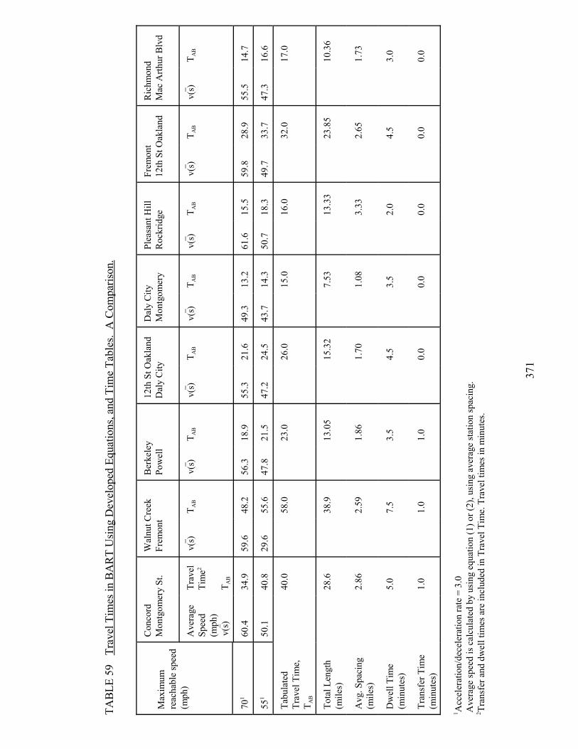
371

TAB

LE 5

9Tr

avel

Tim

es in

BA

RT

Usi

ng D

evel

oped

Equ

atio

ns, a

nd T

ime

Tabl

es.

A C

ompa

rison

.

Max

imum

reac

habl

e sp

eed

(mph

)

Con

cord

M

ontg

omer

y St

.W

alnu

t Cre

ekFr

emon

tB

erke

ley

Pow

ell

12th

St O

akla

ndD

aly

City

Dal

y C

ityM

ontg

omer

yPl

easa

nt H

illR

ockr

idge

Frem

ont

12th

St O

akla

ndR

ichm

ond

Mac

Arth

ur B

lvd

Ave

rage

Spee

d(m

ph)

v(s)

Trav

elTi

me2

T AB

T AB

T AB

T AB

T AB

T AB

T AB

T AB

v(s)

v(s)

v(s)

v(s)

v(s)

v(s)

v(s)

701

60.4

34.9

59.6

48.2

56.3

18.9

55.3

21.6

49.3

13.2

61.6

15.5

59.8

28.9

55.5

14.7

551

50.1

40.8

29.6

55.6

47.8

21.5

47.2

24.5

43.7

14.3

50.7

18.3

49.7

33.7

47.3

16.6

Tabu

late

dTr

avel

Tim

e,T A

B

40.0

58.0

23.0

26.0

15.0

16.0

32.0

17.0

Tota

l Len

gth

(mile

s)

28.6

38.9

13.0

515

.32

7.53

13.3

323

.85

10.3

6

Avg

. Spa

cing

(mile

s)

2.86

2.59

1.86

1.70

1.08

3.33

2.65

1.73

Dw

ell T

ime

(min

utes

) 5.

07.

53.

54.

53.

52.

04.

53.

0

Tran

sfer

Tim

e(m

inut

es)

1.0

1.0

1.0

0.0

0.0

0.0

0.0

0.0

1 Acc

eler

atio

n/de

cele

ratio

n ra

te =

3.0

Ave

rage

spee

d is

cal

cula

ted

by u

sing

equ

atio

n (1

) or (

2), u

sing

ave

rage

stat

ion

spac

ing.

2 Tran

sfer

and

dw

ell t

imes

are

incl

uded

in T

rave

l Tim

e. T

rave

l tim

es in

min

utes

.

372

TB � 60 � Dist / v(s,V/C,F) � ta �N

k�1Vk/60 ,

Bus travel times. In this section equations are developed for buson-vehicle time in mixed traffic: that is, the highway or street capacity is sharedby autos and buses, which in heavy traffic tend to get in each other's way and slowtravel speeds. Besides these volume/ capacity conditions en route, bus travelspeeds are dependent on traffic signalization practices, on-street parking policies,one-waying, and other factors such as the presence of pedestrians and otherdistractions that tend to vary with the location (e.g., residential, downtown) of theroute or link within the metropolitan area.

The on-vehicle time on bus may be expressed as

(18)

where

TB = bus on-vehicle time (minutes);

Dist = linehaul distance (miles);

(s, V/C, F) = average speed evaluated at bus stop spacing s , volumevcapacity ratio V/C , and in location F with given parkingpolicy, signalization, one-way conditions (mph);

ta = boarding/alighting time of one passenger at a bus stop (seconds);

Vk = volume of passengers alighting and/or boarding at stop k(passengers).

The parameters or functions to be determined for applying equation (18)are , and ta . Examining the boarding/alighting time first, for simplicity, itv(�)appears that, on the average, passenger service times range from two seconds(single-coin) to more than eight seconds (multiple zone fares collected by thedriver) per passenger (12).

The boarding times also appear to be somewhat greater than alightingtimes, although at least some of the total dwell time must reflect total passengerexchange and "clearance" to get the bus back to the traffic stream. For currentconditions it is assumed that regardless of the type of payment theboarding/alighting time is 3.0 seconds; this appears to be in agreement withobservations made in the Bay Area and also with values in Table 60.

373

TABLE 60 Approximate Passenger Service Time On and Off Buses

Operation Conditions Time (sec)

Unloading Very little hand baggage and parcels; few transfers 1.5 - 2.5

Moderate amount of hand baggage or many transfers 2.5 - 4

Considerable baggage from racks (intercity runs) 4 - 6

Loadinga Single coin or token fare box 2 - 3

Odd-penny cash fares; multiple-zone fares 3 - 4

Pre-purchased tickets and registration on bus 4 - 6

Multiple-zone fares; cash; including registration on bus 6 - 8

Prepayment before entering bus or pay when leaving bus 1.5 - 2.5

aAdd 1 second where fare receipts are involved.

Source: "Bus Use of Highway--Planning and Design Guidelines," NCHRP Report155, Washington, DC (1975)

The main factor affecting bus on-vehicle time over a given distance is, ofcourse, the average bus speed in the traffic stream. As indicated earlier, bus speedis a function of several variables--volume/ capacity, bus stop frequency,signalization, parking policies, number of lanes, etc. A search of the literature onthe topic turned up one big surprise: there appears to be a total lack of statisticalanalysis of bus speeds under varying operating policies and volume/capacitycircumstances. For this reason somewhat ad hoc methods are employed here tocompute the average bus speed and, hence, the bus on-vehicle time.

The average bus speed is obtained from the average car speed (vC) usingequation (15), by assuming that the average car speed is the maximum speed a buscan attain in any given conditions, and that the bus stop spacing is large enough

374

for buses to obtain this maximum speed. Both of these assumptions arereasonable. Average car speed in turn can be obtained from the Highway CapacityManual using standard assumptions about traffic conditions (e.g., percent trucks,percent right and left turns, etc.) or from the car travel time equations developedearlier for the single "bottleneck" situation. Using the notation defined earlier,and vc is the car speed in prevailing conditions, the bus travel time can then beexpressed as

(19) TB � �s�Dist

60 �

1vc

�

vc

7200s� .05 � �

N

k�1Vk ,

where the first summation is over all intervals between bus stops covering the tripdistance. This equation can be modified to express the approximate bus traveltime over a distance,

(200 TB � TA �(Dist)2

2�s�TA

�

.05Vk�Dist

s,

where the new notation is

TA is the auto travel time over the distance (Dist) under prevailingconditions (e.g., equation (15) or Table 13);

average spacing of bus stops over the distance;s

average number of passengers boarding/alighting at stops.Vk

In equation (20) the second term expresses delay due toacceleration/deceleration and the third term is the delay due to boarding/alightingpassengers.

The use of equation (20) was demonstrated by a test application. Equation(20) was applied to fifteen hypothetical trips between randomly selected originsand destinations. Comparisons were made between tabulated travel times (fromtimetables) network coded travel times, and the calculated travel times from thesupply model. The results are reported in Talvitie and Dehghani (1976).