chapter 4 dam-break ﬂ ood routing - wit press · the well-known malpasset dam-break event shows...

Chapter 4

Dam-break fl ood routing

R. Garcia-Martinez1,2, N. Gonzalez-Ramirez3 & J. O’Brien4

1Applied Research Center, Florida International University, USA2FLO-2D Software, Inc., Pembroke Pines, FL, USA3 Instituto de Mecánica de Fluidos, Universidad Central de Venezuela, Caracas, Venezuela

4FLO-2D Software, Inc., Nutrioso, AZ, USA

Abstract

Dam-break fl ood modelling is the basis for effective fl ood mitigation. One- dimensional (1D) numerical models have been used to simulate dam-break fl oods for more than 25 years. The intrinsic assumptions in 1D models, such as uniform water velocity and constant water surface elevation on each cross-section, fail to provide accurate predictions of fl ood hydraulics, particularly in areas where the fl ow is unconfi ned or fl oodway area relatively fl at. Two-dimensional (2D) models can provide spatially variable velocities and water surface elevations, which better capture the fl oodwave attenuation and overland storage.

This chapter presents RiverFLO-2D: a 2D fi nite-element river and dam-break fl ood-routing model that uses a parallelized explicit time-stepping scheme. We fi rst outline the model spatial discretization using triangular fi nite elements and show details of the time-stepping scheme and its numerical stabil-ity. Then the dying and wetting algorithm in the context of the fi nite- element method is discussed. Several 2D numerical tests show that model results compare very well, not only with simplified solutions, but also with bench-mark experimental measurements and field data. A full 2D application to the well-known Malpasset dam-break event shows that the model accurately replicates f lood wave travel times and water depths for this physically and numerically demanding real case test.

1 Introduction

Dam failures generate a sudden fl ood wave that travels downstream at very high velocities, obliterating almost everything in its path. In almost all cases, bridges, power plants and all infrastructure along the watercourse are destroyed because the fl ood magnitude far exceeds the design fl ood event. For small dams and reservoirs, fl oodwave attenuation limits the downstream extent of the damage.

c04.indd 141c04.indd 141 8/18/2009 10:15:29 AM8/18/2009 10:15:29 AM

www.witpress.com, ISSN 1755-8336 (on-line) WIT Transactions on State of the Art in Science and Engineering, Vol 36, © 2009 WIT Press

doi:10.2495/978-1-84564- 2- /14 9 04

142 DAM-BREAK PROBLEMS, SOLUTIONS AND CASE STUDIES

For large-volume reservoirs in narrow valleys, the fl ood damage can be incurred for many kilometers downstream.

Dam-break fl ood analysis is an essential component of fl ood risk assessment, fl ood hazard delineation, and water resource management. Mathematical models are an essential tool to support studies involving prediction of complex fl ow pat-terns with irregular banks and bathymetry, and overbank fl ood. In the late 20th century, 1D models were the only feasible way to numerically simulate dam-break fl ows (Fread [1]). Unfortunately, the intrinsic assumptions of 1D models of uniform water surface elevation and average velocity on each cross-section do not provide the needed detail to design and analyze dam-break fl oods on valleys that are not confi ned. Although a dam-break fl ood, particularly at or near the dam site, is three-dimensional (3D), two-dimensional (2D) hydrodynamic models are now widely used because of computational effi ciency and relative accuracy in distributing the fl ood volume.

There are a number of 2D depth-averaged models that have been developed and applied for dam-break fl ood routing or fl ood over dry beds. Some models use the fi nite-difference method (Heniche et al. [2], FLO-2D Software [3]), while others use fi nite volumes (Brufau et al. [6]) or fi nite-element methods (Hervouet [7], Garcia et al. [8]). Generally, the application of these models is suffi cient where the channel represents only a minor portion of the total fl ood conveyance. For large rivers with narrow valleys, the use of square grids common to the fi nite-difference methods limits representation of fl oodway geometry. Boundary- fi tted coordinates fi nite-difference models, fi nite-volume models on unstructured grids, and fi nite-element models improve the spatial resolution for complex dam-break fl ood-routing simulations.

The application of fi nite-volume methods using triangular unstructured meshes is expanding (Murillo et al. [9, 10], and Brufau et al. [11]). These models are very attractive options for 2D dam-break fl ood simulations, although they may require some explicit treatment for oscillations arising from the source terms in the shallow water equations (Vazquez-Cendon [12], Garcia-Navarro et al. [13], and Brufau et al. [14]).

The fi nite-element method is a natural choice for river problems because it allows using numerical meshes that adapt to irregular bed and banks, and is backed by a solid mathematical foundation.

This chapter discusses dam-break fl ood routing using RiverFLO-2D: a 2D fi nite-element free surface fl ow and sediment transport model that uses a four-step selective lumping explicit time-stepping scheme to solve the system of ordinary differential equations that results from the application of the Galerkin weighted residual method to the full 2D dynamic wave equations. Unlike other fi nite- element models [4, 5], the model does not require a diffusion term to stabi-lize the solution and the spatial discretization uses linear triangular elements.

Many time integration schemes in the context of fi nite-element methods to solve the unsteady shallow water equations have appeared in the literature. Kawahara et al. [15] presented a 2D shallow water model based on a two-step

c04.indd 142c04.indd 142 8/18/2009 10:15:29 AM8/18/2009 10:15:29 AM


DAM-BREAK FLOOD ROUTING 143

scheme for tsunami wave propagation. However, this scheme showed exces-sive numerical damping due to the use of lumped mass matrix. Later, Kawahara et al. [16] improved the original scheme by implementing the selective lumping algorithm, which substantially reduces the damping effect while maintaining the computational advantages of using lumped mass matrix. Kashiyama et al. [17] proposed a three-step method for the shallow water equations based on the origi-nal Kawahara selective lumping scheme that proved effi cient in further reducing the damping effect while allowing larger time steps. The four-step time- stepping scheme, improves the original Kashiyama three-step method, allowing even larger time steps and enhancing its capability to simulate dam-break fl ooding. To evaluate the stability of the proposed time-stepping scheme, a von Newmann stability analysis is performed. RiverFLO-2D also implements a robust and mass- conservative drying–wetting algorithm that permits modelling regions that get dry and fl ood during the unsteady simulation.

Until recently, 2D dam-break routing models had not taken advantage of the availability of multiple-core processor computers. Most present-day models are still based on sequential codes that do not take advantage of multiple- threading programming techniques. Although some 2D models have been parallelized, they have been confi ned to computer cluster environments that are mostly limited to government agencies or universities, and are often not accessible to many con-sulting engineering companies.

RiverFLO-2D is coded in FORTRAN 95 and was parallelized using OpenMP application programming interface [19]. OpenMP provides extensive functionality to develop shared-memory multiprocessing programs and offers immediate access to multiple-core processors available in dual and quad-core computers, without requiring complex-to-use computer clusters. Unlike most fi nite-element models that are computationally expensive and require simul-taneous solution of matrix systems, RiverFLO-2D element-by-element explicit time-stepping scheme is well suited to effi cient parallelization. Tests in dual- and quad-processor computers indicate that the parallelized RiverFLO-2D model is able to run up to 2.5 faster than the sequential code in single-processor computers.

To verify and validate RiverFLO-2D and demonstrate its capabilities to simu-late dam-break fl ood routing, we follow the verifi cation process recommended by the ASCE 3D Flow Model Verifi cation and Validation Committee [20]. This process involves testing the model with analytical solutions and simplifi ed cases, tests with laboratory experiments, and fi nally comparisons with documented real cases where fi eld data is available. We present a number of tests that include com-parison with idealized comparisons against dam-break laboratory experiments, and application to a real dam-break event. Numerical tests show that RiverFLO-2D model results compare very well, with both simplifi ed solutions and bench-mark experimental measurements. RiverFLO-2D application to the well-known Malpasset dam-break event reveals that the model accurately predicts the wave travel time and water depths.

c04.indd 143c04.indd 143 8/18/2009 10:15:29 AM8/18/2009 10:15:29 AM



2 Governing equations

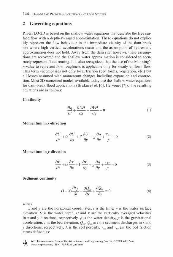
RiverFLO-2D is based on the shallow water equations that describe the free sur-face fl ow with a depth-averaged approximation. These equations do not explic-itly represent the fl ow behaviour in the immediate vicinity of the dam-break site where high vertical accelerations occur and the assumption of hydrostatic approximation does not hold. Away from the dam site, however, these assump-tions are recovered and the shallow water approximation is considered to accu-rately represent fl ood routing. It is also recognized that the use of the Manning’s n-value to represent fl ow roughness is applicable only for steady uniform fl ow. This term encompasses not only local friction (bed forms, vegetation, etc.) but all losses assumed with momentum changes including expansion and contrac-tion. Most 2D numerical models available today use the shallow water equations for dam-break fl ood applications (Brufau et al. [6], Hervouet [7]). The resulting equations are as follows:

Continuity

∂∂

+∂

∂+

∂∂

ηt

UHx

VHy

= 0 (1)

Momentum in x-direction

∂∂

+∂∂

+∂∂

+∂∂

+Ut

UUx

VUy

gx

xη τρb = 0 (2)

Momentum in y-direction

∂∂

+∂∂

+∂∂

+∂∂

+Vt

UVx

VVy

gy

yη τ

ρb = 0

(3)

Sediment continuity

(1 ) = 0−

∂

∂+

∂∂

+∂

∂λ

z

tQx

Q

yf x ys s

(4)

where:x and y are the horizontal coordinates, t is the time, η is the water surface

elevation, H is the water depth, U and V are the vertically averaged velocities in x and y directions, respectively, ρ is the water density, g is the gravitational acceleration, zf is the bed elevation, Qsx, Qsy are the sediment discharges in x and y directions, respectively, λ is the soil porosity, τbx and τby are the bed friction terms defi ned as:

c04.indd 144c04.indd 144 8/18/2009 10:15:29 AM8/18/2009 10:15:29 AM



τbx

gn U U VH

=2 2 2

4/3+

(5)

τby

gn V U VH

=2 2 2

4/3+

(6)

and n is the Manning roughness coeffi cient.

2.1 Sediment transport model

Accounting for sediment transport and mobile bed (degradation and aggradation) is important not only for alluvial river dynamics but also for dam-break fl ood evaluations. It has been documented [7] how dam-break waves often generate considerable bed changes downstream from the dam site.

For projects where mobile bed issues are important, RiverFLO-2D provides several transport formulas to calculate sediment discharge (Stevens and Yang [18]). To illustrate how a sediment transport capacity equation is incorporated into the model, the Meyer–Peter and Muller formula is used as an example.

Sediment discharges in x and y directions are evaluated as follows:

Q Q

UU V

Q QV

U Vx ys s s s=( )

; =( )2 2 1/2 2 2 1/2+ +

(7)

where Qs is the total sediment discharge calculated as:

Q

Qs b c

ss

b c b c

when

when

0

811 2 3 2

τ τ

ρ τ τ τ τγ γ

( ) ≥

(8)

γs and γw are the sediment and water-specifi c weight, respectively, τb is the bed shear stress computed as

τ

γb = ( )

2

1/32 2n

hU V+

(9)

τc is the critical shear stress expressed as

τc = 0.047(γs – γ)Dm

(10)

and Dm is the effective diameter of bed material mixture

D D iii

n

m s b==∑

1 (11)

c04.indd 145c04.indd 145 8/18/2009 10:15:29 AM8/18/2009 10:15:29 AM



where Dsi is the mean grain diameter of the sediment in size fraction i, ib the weight fraction of bed material in fraction i and n the number of size fractions.

2.2 Finite-element discretization

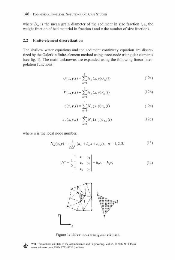
The shallow water equations and the sediment continuity equation are discre-tized by the Galerkin fi nite-element method using three-node triangular elements (see fi g. 1). The main unknowns are expanded using the following linear inter-polation functions:

U x y t N x y U t( , , ) ( , ) ( )

α α

α 1

3

∑

(12a)

V x y t N x y V t( , , ) ( , ) ( )

α α

α 1

3

∑

(12b)

η ηα α

α( , , ) ( , ) ( )x y t N x y t

1

3

∑

(12c)

z x y t N x y z tf f( , , ) ( , ) ( )

α α

α 1

3

∑

(12d)

where α is the local node number,

N x y a b x c yeα α α α α( , ) =

12

( ), = 1,2,3.∆

+ +

(13)

∆ex yx yx y

b c b c=12

111

=1 1

2 2

3 3

2 3 3 2−

(14)

3

2e

e

1

x

y

Figure 1: Three-node triangular element.

c04.indd 146c04.indd 146 8/18/2009 10:15:29 AM8/18/2009 10:15:29 AM



and

a x y x y b y y c x xa x y x y b y y c x

1 2 3 3 2 1 2 3 1 3 2

2 3 1 1 3 2 3 1 2 1

= , = , == , = , =

− − −− − − xx

a x y x y b y y c x x3

3 1 2 2 1 3 1 2 3 2 1= , = , =− − −

(15)

Substituting eqn. (12) in eqns. (1)–(4) and applying the Galerkin weighted residual method, we obtain the following system of ordinary differential equations:

M

d

dtX U H Y V H R He e e e

αββ

αβγ β γ αβγ β γ αβ βη

+ + =

(16)

MdU

dtX U U Y V U N f V

gR G M U

e e e e

efe e

αββ

αβγ β γ αβγ β γ αβγ β γ

αβ β αβ βη

+ + −

+ + = 00 (17)

M

dV

dtX U V Y V V N f U

gS G M V

e e e e

efe e

αββ

αβγ β γ αβγ β γ αβγ β β

αβ β αβ βη

+ + +

+ + = 00 (18)

(1 ) = 0− + +λ αβ

βαβ β αβ βM

dz

dtR Q S Qe f e

xe

xs s

(19)

where:

M N N de

e e

αβ α β αβδ= =12

(1 ) =12

2 1 11 2 11 1 2

∫ +

⎡

⎣

⎢⎢⎢⎢

⎤

⎦

⎥⎥⎥⎥

Ω∆ ∆

(20)

where:

X N NN

xd

b beαβγ α β

γ γαβ

γδ= =24

(1 ) =24

2 1 11 2 11 1 2

∫∂

∂+

⎡

⎣

⎢⎢⎢⎢

⎤

⎦

⎥⎥⎥⎥

Ω

(21)

Y N NN

yd

c ceαβγ α β

γ γαβ

γδ= =24

(1 ) =24

2 1 11 2 11 1 2

∫∂

∂+

⎡

⎣

⎢⎢⎢⎢

⎤

⎦

⎥⎥⎥⎥

Ω

(22)

α =( )1

α =( )2

α =( )3

c04.indd 147c04.indd 147 8/18/2009 10:15:30 AM8/18/2009 10:15:30 AM



N N N N dee

αβγ α β γ β= =60

( )6 2 22 2 12 1 2

,2 2 12 6 21 2 2

∫⎡

⎣

⎢⎢⎢⎢

⎤

⎦

⎥⎥⎥⎥

⎡

⎣

⎢⎢Ω

∆⎢⎢⎢

⎤

⎦

⎥⎥⎥⎥

⎡

⎣

⎢⎢⎢⎢

⎤

⎦

⎥⎥⎥⎥

,2 1 21 2 22 2 6

(23)

R N

N

xd

beαβ α

β β= =6∫

∂

∂ Ω

(24)

S N

N

yd

ceαβ α

β β= =6∫

∂

∂ Ω

(25)

Γ Γve

v e= ∩δ (26)

G

gn U VHf

e =2 2 2

4/3+

(27)

H H

U U

V V

jj

jj

jj

=13

=13

=13

∑

∑

∑

(28)

2.3 Explicit time-stepping scheme

To solve the system of eqns. (16)–(19) we implement an explicit time-stepping scheme that does not require assembly of the global matrices or simultaneous solution of the global algebraic system that is usually required in implicit fi nite-element methods. The solution method involves element-by-element matrix assembly, and consequently, the mesh node numbering does not impact memory requirements or computer time while facilitating code parallelization.

Let us write the system (16)–(19) as

M

d

dtαββ

α βU

F U= ( )−

(29)

where U is the vector of unknowns and F a vector that includes the right-hand terms in the equations. In order to solve eqn. (29), we propose a four-step scheme based on a fractional step decomposition of the following Taylor series expansion for f:

c04.indd 148c04.indd 148 8/18/2009 10:15:30 AM8/18/2009 10:15:30 AM



f t t f t tdf t

dtt d f t

dtt d f t

dtt d

( ) = ( )( )

2( )

6( )

24

2 2

2

3 3

3

4 4

+ + + +

+

∆ ∆∆ ∆

∆ ff tdt

O t( )

( )44+ ∆

(30)

where Δt is the time interval.It can be demonstrated that eqn. (30) can be expressed in the following four-

step fractional-step scheme:

f t

tf t

t df tdt

∆ ∆4 4

⎛

⎝⎜⎜⎜

⎞

⎠⎟⎟⎟⎟ ( )

( )

(31a)

f t

tf t

t df t tdt

∆ ∆ ∆

3 34⎛

⎝⎜⎜⎜

⎞

⎠⎟⎟⎟⎟ ( )

( ( / ))

(31b)

f t

tf t

t df t tdt

∆ ∆ ∆

2 23⎛

⎝⎜⎜⎜

⎞

⎠⎟⎟⎟⎟ ( )

( ( / ))

(31c)

f t t f t t

df t tdt

( ) ( )( ( / ))

∆ ∆∆ 2

(31d)

Applying this scheme to eqn. (29) we obtain the following four-step scheme:

First step

M M

tFn n n

αβ β αβ β α βU U U+ −1/4 =4

( )∆

(32)

Second step

M M

tFn n n

αβ β αβ β α βU U U+ +−1/3 1/4=3

( )∆

(33)

Third step

M M

tFn n n

αβ β αβ β α βU U U+ +−1/2 1/3=2

( )∆

(34)

Fourth step

M M tFn n n

αβ β αβ β α βU U U+ +−1 1/2= ( )∆

(35)

c04.indd 149c04.indd 149 8/18/2009 10:15:30 AM8/18/2009 10:15:30 AM



Defi ning the lumped matrix as:

MM

αββ αβ α β

α β

Σ if if 0 ≠

⎧⎨⎪⎪⎩⎪⎪

(36a)

∆e

3

1 0 00 1 00 0 1

⎛

⎝

⎜⎜⎜⎜⎜⎜⎜

⎞

⎠

⎟⎟⎟⎟⎟⎟⎟⎟

(36b)

and substituting M by M in eqns. (32)–(35) we obtain the following explicit method:

First step

M M

tFn n n

αβ β αβ β α βU U U+ −1/4 =4

( )∆

(37)

Second step

M M

tFn n n

αβ β αβ β α βU U U+ +−1/3 1/4=3

( )∆

(38)

Third step

M M

tFn n n

αβ β αβ β α βU U U+ +−1/2 1/3=2

( )∆

(39)

Fourth step

M M tFn n n

αβ β αβ β α βU U U1 1/2= ( )− +∆

(40)

It has been found [16] that the above scheme artifi cially damps waves in the numerical solution, and hence we adopted the selective lumping approximation used in ref. [16]. This has proved useful to reduce excessive numerical damping. Therefore, defi ning the selective lumping matrix as:

M M Mαβ αβ αβε ε= (1 )+ −

(41)

where ε is a numerical coeffi cient that may vary in the interval [0,1], and substitut-ing M by M in eqns. (37)–(40) we obtain the four-step selective lumping method:

First step

M M

tFij j

nij j

ni j

nU U U+ −1/4 =4

( ) ∆

(42)

c04.indd 150c04.indd 150 8/18/2009 10:15:30 AM8/18/2009 10:15:30 AM



Second step

M M

tFij j

nij j

ni j

nU U U+ +−1/3 1/4=3

( ) ∆

(43)

Third step

M M

tFij j

nij j

ni j

nU U U+ +−1/2 1/3=2

( ) ∆

(44)

Fourth step

M M tFij j

nij j

ni j

nU U U+ +−1 1/2= ( ) ∆

(45)

2.4 Stability analysis

To evaluate the stability of the proposed four-step scheme and obtain estimates for theoretical maximum time steps, we will consider the following one-dimensional (1D) shallow water equations:

∂∂

+∂∂

Ut

gxη

0

(46a)

∂∂

∂∂

ηt

hUx

0

(46b)

where U is the water velocity, η the water elevation, g the gravitational accelera-tion, and h the water depth. Assuming, linear two-node 1D fi nite elements, we obtain the following discretized equations for the ith node:

First step

U U U U

g

in

in

in

in

in

in

+− +

+ −

−+

++

−

− −⎛

⎝⎜⎜

1/41 1

1 1

=1

62

31

6

412

12

ε ε ε

µη η⎜⎜

⎞

⎠⎟⎟⎟⎟

(47)

η η η η

µ

ε ε εin

in

in

in

in

inh U U

+− +

+ −

−+

++

−

− −⎛

⎝⎜⎜

1/41 1

1 1

=1

62

31

6

412

12⎜⎜

⎞

⎠⎟⎟⎟⎟

(48)

c04.indd 151c04.indd 151 8/18/2009 10:15:30 AM8/18/2009 10:15:30 AM



Second step

U U U U

g

in

in

in

in

in

in

+− +

++

−

−+

++

−

− −

1/31 1

11/4

1

=1

62

31

6

312

12

ε ε ε

µη η ++⎛

⎝⎜⎜⎜

⎞

⎠⎟⎟⎟⎟

1/4

(49)

η η η η

µ

ε ε εin

in

in

in

in

inh U U

+− +

++

−

−+

++

−

− −

1/31 1

11/4

1

=1

62

31

6

312

12

++⎛

⎝⎜⎜⎜

⎞

⎠⎟⎟⎟⎟

1/4

(50)

Third step

U U U U gin

in

in

in

in

in+

− + ++

−−

++

+− − −1/2

1 1 11/3

1=1

62

31

6 212

12

ε ε ε µη η ++⎛

⎝⎜⎜⎜

⎞

⎠⎟⎟⎟⎟

1/3

(51)

η η η ηµε ε ε

in

in

in

in

in

inh U U+

− + ++

−−

++

+−

− −1/21 1 1

1/31=

16

23

16 2

12

12

++⎛

⎝⎜⎜⎜

⎞

⎠⎟⎟⎟⎟

1/3

(52)

Fourth step

U U U U gin

in

in

in

in

in=

16

23

16

12

121 1 1

1/211/2−

++

+− − −− + +

+−+ε ε ε µ η η

(53)

η η η η µε ε εin

in

in

in

in

inh U U=

16

23

16

12

121 1 1

1/211/2−

++

+−

− −⎛

− + ++

−+

⎝⎝⎜⎜⎜

⎞

⎠⎟⎟⎟⎟

(54)

where:

µ =

∆∆

tx

(55)

Now consider a solution of the following type

U P ein n I i= ω

(56)

η ωin n I iQ e= (57)

where I = 1− , P and Q are the amplifi cation factors for the velocity and water elevation, respectively. Introducing eqns. (56) and (57) in eqns. (47)–(54) we obtain the following matrix system:

c04.indd 152c04.indd 152 8/18/2009 10:15:30 AM8/18/2009 10:15:30 AM



P

Q

P

Q

P

Q

P

Q

n

n

n

n

n

n

n

n

+

+

+

+

+

+

+

+

⎡

⎣

⎢⎢⎢⎢⎢⎢⎢⎢⎢⎢⎢⎢

1/4

1/4

1/3

1/3

1/2

1/2

1

1

⎢⎢⎢⎢⎢⎢⎢

⎤

⎦

⎥⎥⎥⎥⎥⎥⎥⎥⎥⎥⎥⎥⎥⎥⎥⎥⎥⎥

=

0 0 0 0 0 0

0 0 0 0 0 0

0 0 0

14

14

13

a gb

hb a

a gb 00 0 0

0 0 0 0 0 0

0 0 0 0 0 0

0 0 0 0 0 0

0 0 0 0 0 0

0 0 0 0 0 0

13

12

12

a hb

a gb

a hb

a gb

a hb

⎡

⎣

⎢⎢⎢⎢⎢⎢⎢⎢⎢⎢⎢⎢⎢⎢⎢⎢⎢⎢⎢

⎤

⎦

⎥⎥⎥⎥⎥⎥⎥⎥⎥⎥⎥⎥⎥⎥⎥⎥⎥⎥

+

+

+

P

Q

P

Q

P

n

n

n

n

n

1/4

1/4

1//3

1/3

1/2

1/2

Q

P

Q

n

n

n

+

+

+

⎡

⎣

⎢⎢⎢⎢⎢⎢⎢⎢⎢⎢⎢⎢⎢⎢⎢⎢⎢⎢

⎤

⎦

⎥⎥⎥⎥⎥⎥⎥⎥⎥⎥⎥⎥⎥⎥⎥⎥⎥⎥⎥

(58)

where:

a

e e=

23

13

++

−cos ω

(59)

b I= − µ ωsin (60)

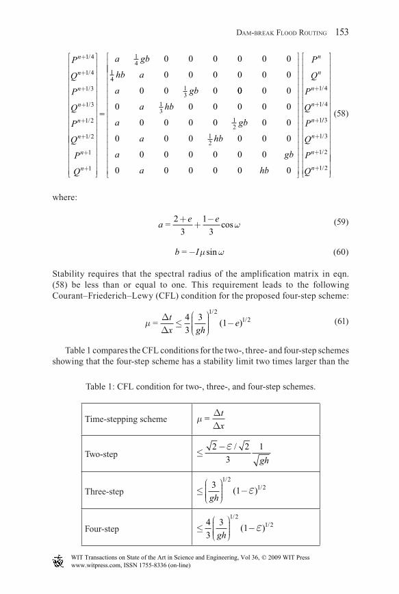
Stability requires that the spectral radius of the amplifi cation matrix in eqn. (58) be less than or equal to one. This requirement leads to the followingCourant–Friederich–Lewy (CFL) condition for the proposed four-step scheme:

µ =43

3(1 )

1/21/2∆

∆tx gh

e≤⎛

⎝⎜⎜⎜⎜

⎞

⎠⎟⎟⎟⎟

−

(61)

Table 1 compares the CFL conditions for the two-, three- and four-step schemes showing that the four-step scheme has a stability limit two times larger than the

Table 1: CFL condition for two-, three-, and four-step schemes.

Time-stepping scheme µ =∆∆

tx

Two-step ≤−2 / 2

31εgh

Three-step ≤⎛

⎝⎜⎜⎜⎜

⎞

⎠⎟⎟⎟⎟

−3

(1 )1/2

1/2

ghε

Four-step ≤⎛

⎝⎜⎜⎜⎜

⎞

⎠⎟⎟⎟⎟

−43

3(1 )

1/21/2

ghε

c04.indd 153c04.indd 153 8/18/2009 10:15:30 AM8/18/2009 10:15:30 AM



two-step scheme and 1.33 times larger than the three-step scheme. It should be kept in mind that these limits correspond to the linear stability analysis, and in practical applications, the actual time steps allowed will normally be different.

3 Numerical treatment of dry bed

RiverFLO-2D is able to simulate the drying and wetting of the bed. This model capability is important when modelling dam-break fl ooding as the river valley is initially dry; then the bed gets fl ooded as the wave progresses downstream. The bed dries again as the wave recedes.

RiverFLO-2D drying and wetting algorithm is an improved version from the one originally proposed by Kawahara and Umetsu [23] and later by Umetsu and Matsumoto [22] in the fi nite-element context. In this approach, the fi nite-element mesh is generated so that it will cover the whole region that is expected to be fl ooded. The wetting–drying algorithm is as follows:

1. At the beginning of each time step all elements are evaluated to see if they are wet or dry. A completely dry element is defi ned when all nodal depths are less than a user-defi ned minimum depth or tolerance value Hmin, that can be zero. A partially dry element has at least one node, where depth is less than or equal to Hmin.

2. If the element is completely dry the following equations are solved:

∂∂

∂∂

∂∂

ηt

Ut

Vt

= 0; = 0; = 0

(62)

These equations are discretized and solved using the fi nite-element proce-dure described above. Also, for these dry elements velocity components are set to zero for all nodes on the element.

3. If an element is partially dry, the full equations are solved and velocity compo-nents are set to zero for all nodes on the element.

4. Water surface elevations are not modifi ed for dry elements.

A similar algorithm was implemented by Garcia et al. [8], which worked adequately when the dry areas occurred over a relatively small portion of the whole mesh, but showed some mass conservation errors when large areas became dry. The example applications presented later in this chapter indicate that the proposed method generates stable numerical solutions with no spurious velocities over dry areas and minimal mass conservation errors.

4 OpenMP parallelization

The OpenMP Application Program Interface (API) supports multiplatform shared-memory parallel programming in C/C++ and Fortran on all architectures,

c04.indd 154c04.indd 154 8/18/2009 10:15:30 AM8/18/2009 10:15:30 AM



including MAC OS, Unix, and Windows NT platforms [19]. OpenMP is portable and scalable, and provides instructions to parallelized existing serial codes to run in shared-memory platforms ranging from affordable and widely available multiple-core computers to supercomputers.

RiverFLO-2D serial code was parallelized using OpenMP directives avail-able in the Intel Visual Fortran compiler version 11.0. Preliminary tests show that the model can run up to 2.5 faster in quad-core processors.

5 Testing RiverFLO-2D model

Numerical fl ood routing models are commonly tested by predicted hydraulic results directly to measured fi eld data and observations. Once the fi eld data is reasonably replicated, the model developer or the user considers that the model is validated. This validation approach is not always satisfi ed and the results can be skewed or fi ltered to the user’s benefi t; this method has often been abused and has raised doubts about its adequacy [20]. Recently ASCE Task Force Committee for 3D Flow Model Verifi cation and Validation [20] reviewed fl ow model testing and recommended an approach for model validation. To verify and validate RiverFLO-2D the verifi cation process recommended by ASCE Committee was followed. The process involves testing the model with ana-lytical solutions and simplifi ed cases, tests with laboratory experiments, and fi nally comparisons with documented real cases, where fi eld data is avail-able. A previous publication (Garcia et al. [8]) has reported on RiverFLO-2D tests using benchmark analytical solutions on wet beds. In this section, we present further tests to verify that RiverFLO-2D is able to simulate fl ow over initially dry beds using simplifi ed cases and experimental measurements fordam-break fl ows.

5.1 Test for wet–dry capabilities under static conditions

The goal of this test is to evaluate the model performance under static conditions, where one part of the fi nite-element mesh is dry and has irregular bed elevations and relatively steep slopes. Dry steep slope elements may pose a severe numerical problem because if handled incorrectly, the 2D gravity term in the equations can generate erratic fl ow. Starting with a static initial water depth that leaves part of the bed dry, a properly working dry bed algorithm should preserve the initial static con-ditions, minimize mass conservation errors and be free from erroneous velocities.

It appears that this numerical experiment was fi rst proposed by Brufau et al. [11]. The problem consists of a square pool 1 m × 1 m with a central bump on the bottom defi ned by the following formula:

z x y x y( , ) = 0, 0.25 512

12

2 2

max − −⎛⎝⎜⎜⎜

⎞⎠⎟⎟⎟ + −

⎛⎝⎜⎜⎜

⎞⎠⎟⎟⎟

⎡

⎣

⎢⎢⎢

⎤

⎦

⎥⎥⎥⎥

⎧⎨⎪⎪⎪

⎩⎪⎪⎪

⎫⎬⎪⎪⎪

⎭⎪⎪⎪

(63)

c04.indd 155c04.indd 155 8/18/2009 10:15:30 AM8/18/2009 10:15:30 AM


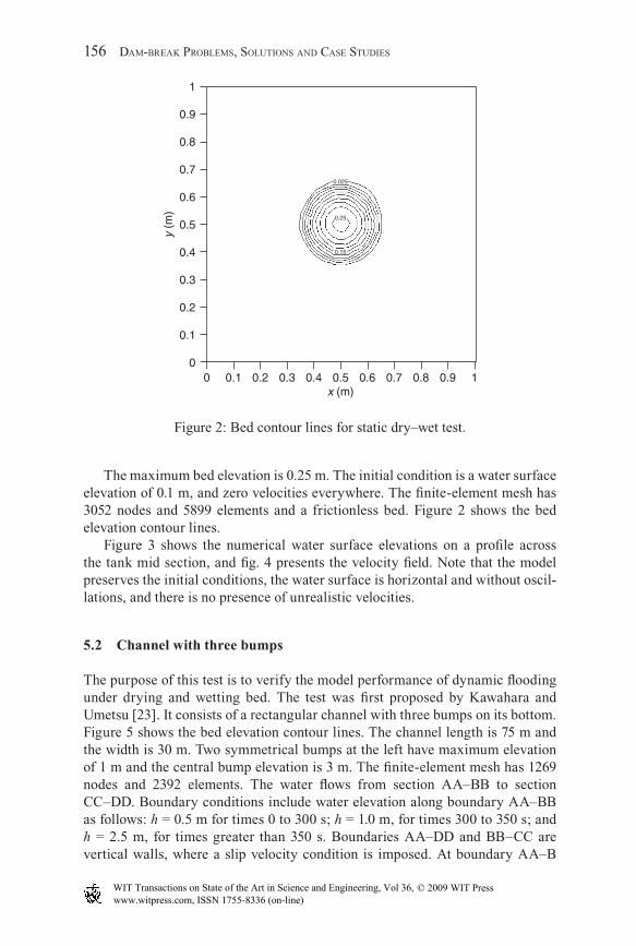
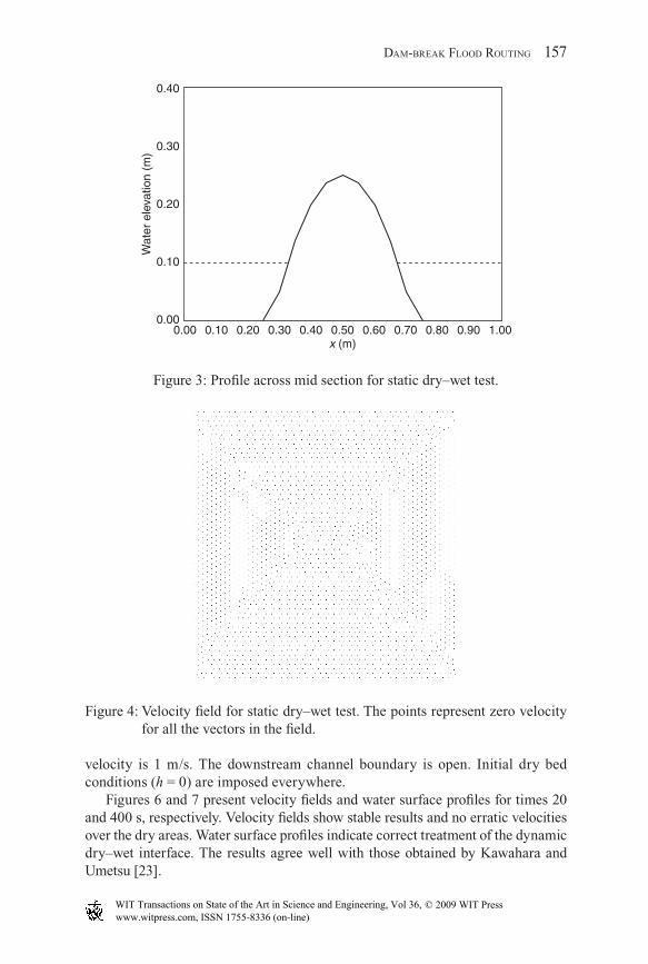
The maximum bed elevation is 0.25 m. The initial condition is a water surface elevation of 0.1 m, and zero velocities everywhere. The fi nite-element mesh has 3052 nodes and 5899 elements and a frictionless bed. Figure 2 shows the bed elevation contour lines.

Figure 3 shows the numerical water surface elevations on a profi le across the tank mid section, and fi g. 4 presents the velocity fi eld. Note that the model preserves the initial conditions, the water surface is horizontal and without oscil-lations, and there is no presence of unrealistic velocities.

5.2 Channel with three bumps

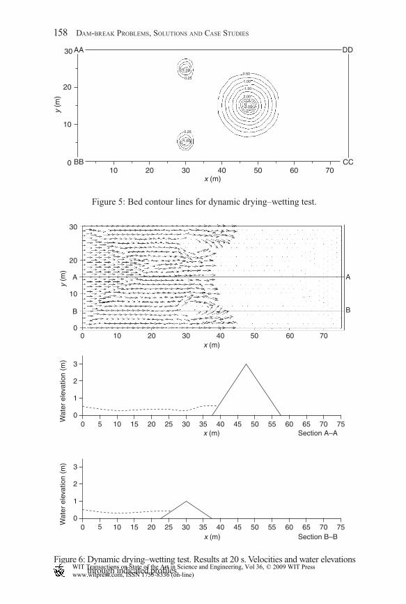
The purpose of this test is to verify the model performance of dynamic fl ooding under drying and wetting bed. The test was fi rst proposed by Kawahara and Umetsu [23]. It consists of a rectangular channel with three bumps on its bottom. Figure 5 shows the bed elevation contour lines. The channel length is 75 m and the width is 30 m. Two symmetrical bumps at the left have maximum elevation of 1 m and the central bump elevation is 3 m. The fi nite-element mesh has 1269 nodes and 2392 elements. The water fl ows from section AA–BB to section CC–DD. Boundary conditions include water elevation along boundary AA–BB as follows: h = 0.5 m for times 0 to 300 s; h = 1.0 m, for times 300 to 350 s; and h = 2.5 m, for times greater than 350 s. Boundaries AA–DD and BB–CC are vertical walls, where a slip velocity condition is imposed. At boundary AA–B

00

0.1

0.1

0.2

0.2

0.3

0.3

0.4

0.4

0.025

0.25

0.15

0.5

0.5

x (m)

y (m

)

0.6

0.6

0.7

0.7

0.8

0.9

1

0.8 0.9 1

Figure 2: Bed contour lines for static dry–wet test.


c04.indd 156c04.indd 156 8/18/2009 10:15:30 AM8/18/2009 10:15:30 AM



0.40

0.30

0.20

Wat

er e

leva

tion

(m)

0.10

0.000.00 0.10 0.20 0.30 0.40 0.50

x (m)0.60 0.70 0.80 0.90 1.00

Figure 3: Profi le across mid section for static dry–wet test.

Figure 4: Velocity fi eld for static dry–wet test. The points represent zero velocity for all the vectors in the fi eld.

velocity is 1 m/s. The downstream channel boundary is open. Initial dry bed conditions (h = 0) are imposed everywhere.

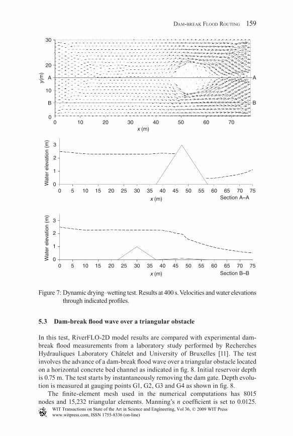
Figures 6 and 7 present velocity fi elds and water surface profi les for times 20 and 400 s, respectively. Velocity fi elds show stable results and no erratic velocities over the dry areas. Water surface profi les indicate correct treatment of the dynamic dry–wet interface. The results agree well with those obtained by Kawahara and Umetsu [23].

c04.indd 157c04.indd 157 8/18/2009 10:15:30 AM8/18/2009 10:15:30 AM


30

20

10

B

00 10

00

1

Wat

er e

leva

tion

(m)

2

3

5 10 15 20 25 30 35 40 45 50 55 60 65 70 75

20 30 40x (m)

x (m) Section A–A

50 60 70

A

B

A

y (m

)

00

1

Wat

er e

leva

tion

(m)

2

3

5 10 15 20 25 30 35 40 45 50 55 60 65 70 75x (m) Section B–B

Figure 6: Dynamic drying–wetting test. Results at 20 s. Velocities and water elevations through indicated profi les.

30

20

10

0 BB10 20 30

0.25

0.250.50

1.00

1.50

2.00

3.00

1.00

1.00

40 50 60 70CC

DDAA

x (m)

y (m

)

Figure 5: Bed contour lines for dynamic drying–wetting test.


c04.indd 158c04.indd 158 8/18/2009 10:15:30 AM8/18/2009 10:15:30 AM



5.3 Dam-break fl ood wave over a triangular obstacle

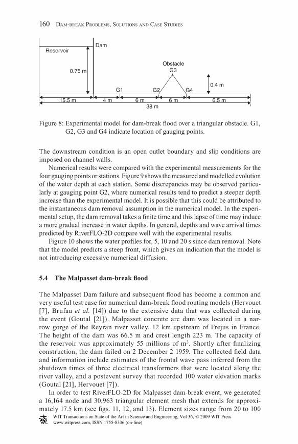
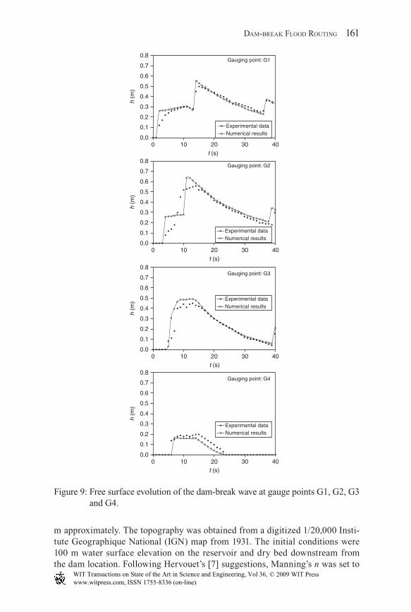
In this test, RiverFLO-2D model results are compared with experimental dam-break fl ood measurements from a laboratory study performed by Recherches Hydrauliques Laboratory Châtelet and University of Bruxelles [11]. The test involves the advance of a dam-break fl ood wave over a triangular obstacle located on a horizontal concrete bed channel as indicated in fi g. 8. Initial reservoir depth is 0.75 m. The test starts by instantaneously removing the dam gate. Depth evolu-tion is measured at gauging points G1, G2, G3 and G4 as shown in fi g. 8.

The fi nite-element mesh used in the numerical computations has 8015 nodes and 15,232 triangular elements. Manning’s n coeffi cient is set to 0.0125.

00W

ater

ele

vatio

n (m

)W

ater

ele

vatio

n (m

)

1

2

3

5 10 15 20 25 30 35

x (m)

40 45 50 55 60 65Section B–B

70 75

00

1

2

3

00

B

10

y(m

)

A

20

30

10 20 30 40x (m)

50 60 70

B

A

5 10 15 20 25 30 35

x (m)

40 45 50 55 60 65Section A–A

70 75

Figure 7: Dynamic drying–wetting test. Results at 400 s. Velocities and water elevations through indicated profi les.

c04.indd 159c04.indd 159 8/18/2009 10:15:31 AM8/18/2009 10:15:31 AM


Reservoir

0.75 m

Dam

G1 G2

G3

G4

Obstacle

0.4 m

6.5 m6 m6 m4 m15.5 m38 m

Figure 8: Experimental model for dam-break fl ood over a triangular obstacle. G1, G2, G3 and G4 indicate location of gauging points.

The downstream condition is an open outlet boundary and slip conditions are imposed on channel walls.

Numerical results were compared with the experimental measurements for the four gauging points or stations. Figure 9 shows the measured and modelled evolution of the water depth at each station. Some discrepancies may be observed particu-larly at gauging point G2, where numerical results tend to predict a steeper depth increase than the experimental model. It is possible that this could be attributed to the instantaneous dam removal assumption in the numerical model. In the experi-mental setup, the dam removal takes a fi nite time and this lapse of time may induce a more gradual increase in water depths. In general, depths and wave arrival times predicted by RiverFLO-2D compare well with the experimental results.

Figure 10 shows the water profi les for, 5, 10 and 20 s since dam removal. Note that the model predicts a steep front, which gives an indication that the model is not introducing excessive numerical diffusion.

5.4 The Malpasset dam-break fl ood

The Malpasset Dam failure and subsequent fl ood has become a common and very useful test case for numerical dam-break fl ood routing models (Hervouet [7], Brufau et al. [14]) due to the extensive data that was collected during the event (Goutal [21]). Malpasset concrete arc dam was located in a nar-row gorge of the Reyran river valley, 12 km upstream of Frejus in France. The height of the dam was 66.5 m and crest length 223 m. The capacity of the reservoir was approximately 55 millions of m3. Shortly after fi nalizing construction, the dam failed on 2 December 2 1959. The collected fi eld data and information include estimates of the frontal wave pass inferred from the shutdown times of three electrical transformers that were located along the river valley, and a postevent survey that recorded 100 water elevation marks (Goutal [21], Hervouet [7]).

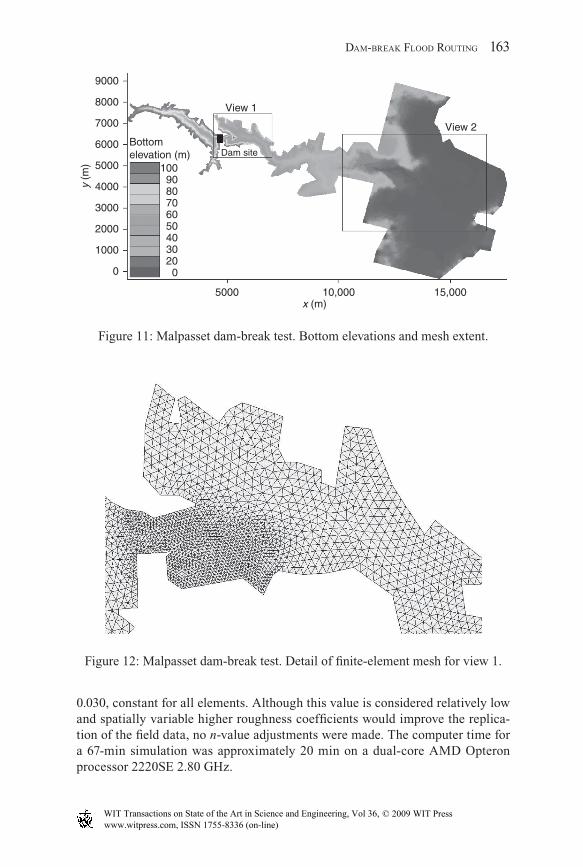
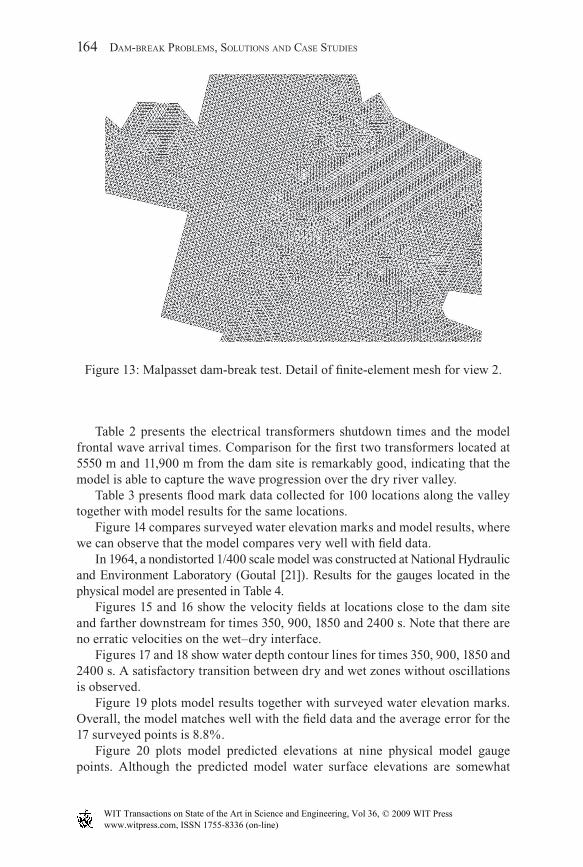
In order to test RiverFLO-2D for Malpasset dam-break event, we generated a 16,164 node and 30,963 triangular element mesh that extends for approxi-mately 17.5 km (see fi gs. 11, 12, and 13). Element sizes range from 20 to 100


c04.indd 160c04.indd 160 8/18/2009 10:15:31 AM8/18/2009 10:15:31 AM



m approximately. The topography was obtained from a digitized 1/20,000 Insti-tute Geographique National (IGN) map from 1931. The initial conditions were 100 m water surface elevation on the reservoir and dry bed downstream from the dam location. Following Hervouet’s [7] suggestions, Manning’s n was set to

0

0.8

0.7

0.6

0.5

0.4

h (m

)

0.3

0.2

0.1

0.010 20

t (s)30

Experimental dataNumerical results

40

Gauging point: G1

0

0.8

0.7

0.6

0.5

0.4

h (m

)

0.3

0.2

0.1

0.010 20

t (s)30 40

Gauging point: G2

0

0.8

0.7

0.6

0.5

0.4

h (m

)

0.3

0.2

0.1

0.010 20

t (s)30 40

Gauging point: G3

0

0.8

0.7

0.6

0.5

0.4

h (m

)

0.3

0.2

0.1

0.010 20

t (s)30 40

Gauging point: G4




Figure 9: Free surface evolution of the dam-break wave at gauge points G1, G2, G3 and G4.

c04.indd 161c04.indd 161 8/18/2009 10:15:31 AM8/18/2009 10:15:31 AM


0

0.8

0.7

0.6

0.5

0.4h

(m)

0.3

0.2

0.1

0.010 20 30

Surface water elevationChannel bed

40

T 3 s

x (m)

0

0.8

0.7

0.6

0.5

0.4

h (m

)

0.3

0.2

0.1

0.010 20 30


40

T 5 s

x (m)

0

0.8

0.7

0.6

0.5

0.4

h (m

)

0.3

0.2

0.1

0.010 20 30


40

T 10 s

x (m)

0

0.8

0.7

0.6

0.5

0.4

h (m

)

0.3

0.2

0.1

0.010 20 30


40

T 20 s

x (m)

Figure 10: Numerical water surface profi le for dam-break wave at 3 s, 5, 10 and 20 s.


c04.indd 162c04.indd 162 8/18/2009 10:15:31 AM8/18/2009 10:15:31 AM



0.030, constant for all elements. Although this value is considered relatively low and spatially variable higher roughness coeffi cients would improve the replica-tion of the fi eld data, no n-value adjustments were made. The computer time for a 67-min simulation was approximately 20 min on a dual-core AMD Opteron processor 2220SE 2.80 GHz.

9000

8000

7000

Bottomelevation (m)

6000

5000

4000

3000

2000

1000

5000 10,000 15,000

0

y (m

)

x (m)

1009080706050403020

0

View 1

View 2

Dam site

Figure 11: Malpasset dam-break test. Bottom elevations and mesh extent.

Figure 12: Malpasset dam-break test. Detail of fi nite-element mesh for view 1.

c04.indd 163c04.indd 163 8/18/2009 10:15:31 AM8/18/2009 10:15:31 AM



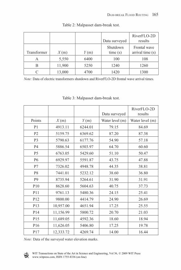
Table 2 presents the electrical transformers shutdown times and the model frontal wave arrival times. Comparison for the fi rst two transformers located at 5550 m and 11,900 m from the dam site is remarkably good, indicating that the model is able to capture the wave progression over the dry river valley.

Table 3 presents fl ood mark data collected for 100 locations along the valley together with model results for the same locations.

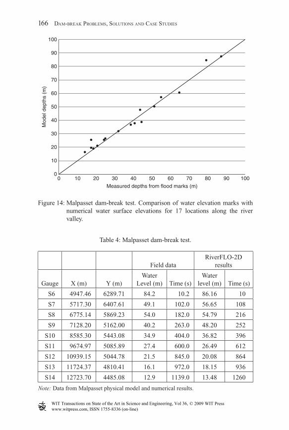
Figure 14 compares surveyed water elevation marks and model results, where we can observe that the model compares very well with fi eld data.

In 1964, a nondistorted 1/400 scale model was constructed at National Hydraulic and Environment Laboratory (Goutal [21]). Results for the gauges located in the physical model are presented in Table 4.

Figures 15 and 16 show the velocity fi elds at locations close to the dam site and farther downstream for times 350, 900, 1850 and 2400 s. Note that there are no erratic velocities on the wet–dry interface.

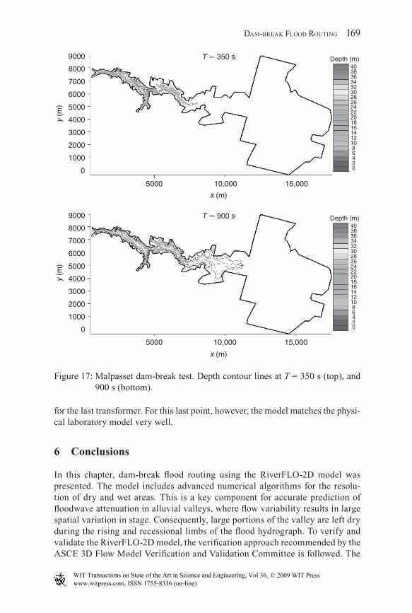
Figures 17 and 18 show water depth contour lines for times 350, 900, 1850 and 2400 s. A satisfactory transition between dry and wet zones without oscillations is observed.

Figure 19 plots model results together with surveyed water elevation marks. Overall, the model matches well with the fi eld data and the average error for the 17 surveyed points is 8.8%.

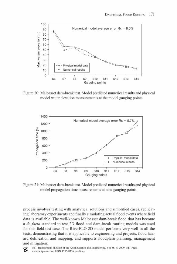
Figure 20 plots model predicted elevations at nine physical model gauge points. Although the predicted model water surface elevations are somewhat

Figure 13: Malpasset dam-break test. Detail of fi nite-element mesh for view 2.

c04.indd 164c04.indd 164 8/18/2009 10:15:31 AM8/18/2009 10:15:31 AM



Data surveyedRiverFLO-2D

results

Points X (m) Y (m) Water level (m) Water level (m)

P1 4913.11 6244.01 79.15 84.69

P2 5159.75 6369.62 87.20 87.38

P3 5790.63 6177.76 54.90 57.18

P4 5886.54 6503.97 64.70 60.60

P5 6763.05 5429.60 51.10 50.47

P6 6929.97 5591.87 43.75 47.88

P7 7326.02 4948.78 44.35 38.81

P8 7441.01 5232.12 38.60 36.80

P9 8735.94 5264.61 31.90 31.91

P10 8628.60 5604.63 40.75 37.73

P11 9761.13 5480.36 24.15 25.41

P12 9800.00 4414.79 24.90 26.69

P13 10,957.00 4651.94 17.25 25.55

P14 11,156.99 5800.72 20.70 21.03

P15 11,689.05 4592.36 18.60 18.94

P16 11,626.05 5406.80 17.25 19.78

P17 12,333.72 4269.74 14.00 16.44

Note: Data of the surveyed water elevation marks.

Table 3: Malpasset dam-break test.

Data surveyedRiverFLO-2D

results

Transformer X (m) Y (m)Shutdown time (s)

Frontal wave arrival time (s)

A 5,550 6400 100 108

B 11,900 5250 1240 1260

C 13,000 4700 1420 1300

Note: Data of electric transformers shutdown and RiverFLO-2D frontal wave arrival times.


c04.indd 165c04.indd 165 8/18/2009 10:15:32 AM8/18/2009 10:15:32 AM



00

10

20

30

40

50

Mod

el d

epth

s (m

)

60

70

80

90

100

10 20 30 40 50

Measured depths from flood marks (m)

60 70 80 90 100

Figure 14: Malpasset dam-break test. Comparison of water elevation marks with numerical water surface elevations for 17 locations along the river valley.


Field dataRiverFLO-2D

results

Gauge X (m) Y (m)Water

Level (m) Time (s)Water

level (m) Time (s)

S6 4947.46 6289.71 84.2 10.2 86.16 10

S7 5717.30 6407.61 49.1 102.0 56.65 108

S8 6775.14 5869.23 54.0 182.0 54.79 216

S9 7128.20 5162.00 40.2 263.0 48.20 252

S10 8585.30 5443.08 34.9 404.0 36.82 396

S11 9674.97 5085.89 27.4 600.0 26.49 612

S12 10939.15 5044.78 21.5 845.0 20.08 864

S13 11724.37 4810.41 16.1 972.0 18.15 936

S14 12723.70 4485.08 12.9 1139.0 13.48 1260

Note: Data from Malpasset physical model and numerical results.

c04.indd 166c04.indd 166 8/18/2009 10:15:32 AM8/18/2009 10:15:32 AM



T 350 s

T 900 s

20 m/s

15 m/s

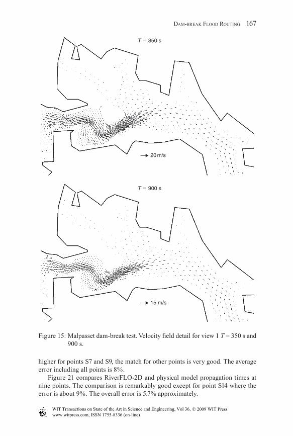
Figure 15: Malpasset dam-break test. Velocity fi eld detail for view 1 T = 350 s and 900 s.

higher for points S7 and S9, the match for other points is very good. The average error including all points is 8%.

Figure 21 compares RiverFLO-2D and physical model propagation times at nine points. The comparison is remarkably good except for point S14 where the error is about 9%. The overall error is 5.7% approximately.

c04.indd 167c04.indd 167 8/18/2009 10:15:32 AM8/18/2009 10:15:32 AM



T 1850 s

T 2400 s

10 m/s

10 m/s

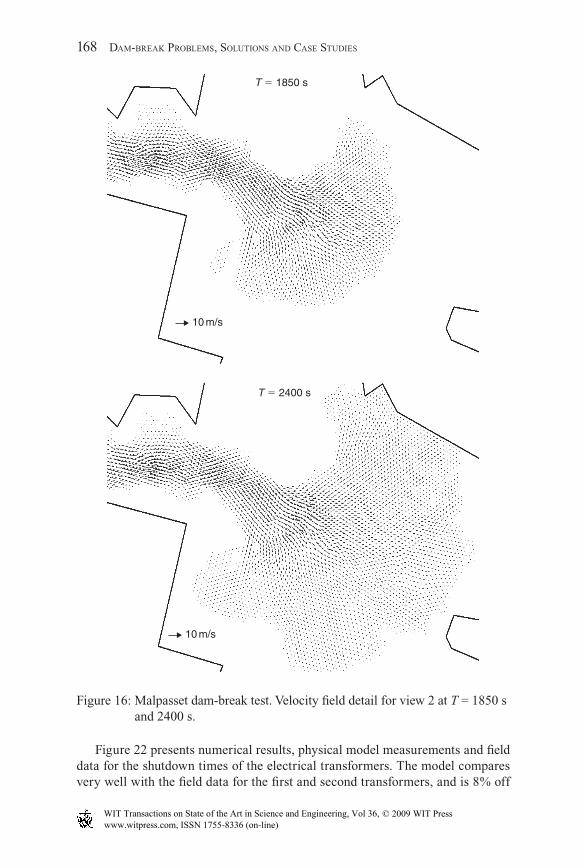
Figure 16: Malpasset dam-break test. Velocity fi eld detail for view 2 at T = 1850 s and 2400 s.

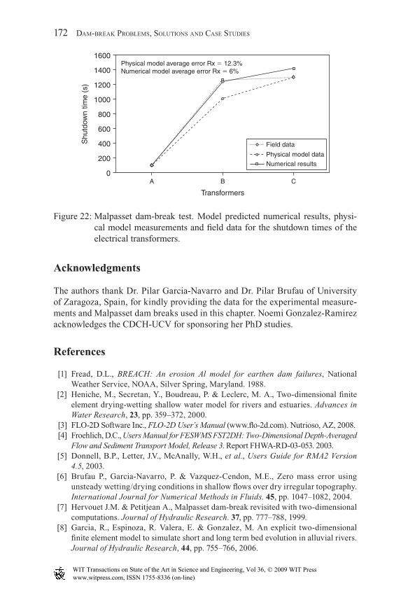
Figure 22 presents numerical results, physical model measurements and fi eld data for the shutdown times of the electrical transformers. The model compares very well with the fi eld data for the fi rst and second transformers, and is 8% off

c04.indd 168c04.indd 168 8/18/2009 10:15:32 AM8/18/2009 10:15:32 AM



for the last transformer. For this last point, however, the model matches the physi-cal laboratory model very well.

6 Conclusions

In this chapter, dam-break fl ood routing using the RiverFLO-2D model was presented. The model includes advanced numerical algorithms for the resolu-tion of dry and wet areas. This is a key component for accurate prediction of fl oodwave attenuation in alluvial valleys, where fl ow variability results in large spatial variation in stage. Consequently, large portions of the valley are left dry during the rising and recessional limbs of the fl ood hydrograph. To verify and validate the RiverFLO-2D model, the verifi cation approach recommended by the ASCE 3D Flow Model Verifi cation and Validation Committee is followed. The

9000

8000

7000

6000

5000

4000

3000

2000

1000

0

y (m

)

5000 10,000

x (m)

15,000

T 350 s Depth (m)4038363432302826242220181614121086420

9000

8000

7000

6000

5000

4000

3000

2000

1000

0

y (m

)

5000 10,000

x (m)

15,000

T 900 s Depth (m)4038363432302826242220181614121086420

Figure 17: Malpasset dam-break test. Depth contour lines at T = 350 s (top), and 900 s (bottom).

c04.indd 169c04.indd 169 8/18/2009 10:15:32 AM8/18/2009 10:15:32 AM


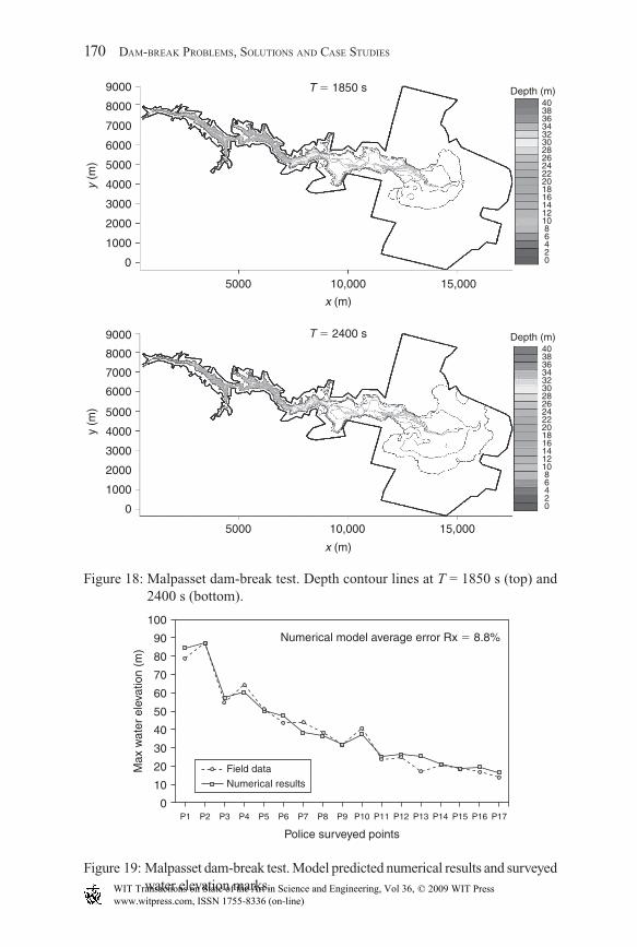
Figure 18: Malpasset dam-break test. Depth contour lines at T = 1850 s (top) and 2400 s (bottom).

9000

8000

7000

6000

5000

4000

3000

2000

1000

0

y (m

)

5000 10,000

x (m)

15,000

T 1850 s Depth (m)4038363432302826242220181614121086420

9000

8000

7000

6000

5000

4000

3000

2000

1000

0

y (m

)

5000 10,000

x (m)

15,000

T 2400 s Depth (m)4038363432302826242220181614121086420

0

10

20

30

40

50

60

70

80

90

100

Max

wat

er e

leva

tion

(m)

P1 P2 P3

Field data

Numerical results

P4 P5 P6 P7 P8

Police surveyed points

P9 P10 P11 P12 P13 P14 P15 P16 P17

Numerical model average error Rx 8.8%

Figure 19: Malpasset dam-break test. Model predicted numerical results and surveyed water elevation marks.


c04.indd 170c04.indd 170 8/18/2009 10:15:32 AM8/18/2009 10:15:32 AM



process involves testing with analytical solutions and simplifi ed cases, replicat-ing laboratory experiments and fi nally simulating actual fl ood events where fi eld data is available. The well-known Malpasset dam-break fl ood that has become a de facto standard to test 2D fl ood and dam-break routing models was used for this fi eld test case. The RiverFLO-2D model performs very well in all the tests, demonstrating that it is applicable to engineering and projects, fl ood haz-ard delineation and mapping, and supports fl oodplain planning, management and mitigation.

0

10

20

30

40

50

60

70

80

90

100

Max

wat

ser

elev

atio

n (m

)


Physical model data

Numerical results

S6 S7 S8 S9 S10 S11 S12 S13Gauging points

S14

Figure 20: Malpasset dam-break test. Model predicted numerical results and physical model water elevation measurements at the model gauging points.

0

200

400

600

800

1000

1200

1400

Pro

paga

tion

time

(s)

S6 S7 S8 S9 S10 S11 S12 S13Gauging points

S14


Physical model data

Numerical results

Figure 21: Malpasset dam-break test. Model predicted numerical results and physical model propagation time measurements at nine gauging points.

c04.indd 171c04.indd 171 8/18/2009 10:15:32 AM8/18/2009 10:15:32 AM



Acknowledgments

The authors thank Dr. Pilar Garcia-Navarro and Dr. Pilar Brufau of University of Zaragoza, Spain, for kindly providing the data for the experimental measure-ments and Malpasset dam breaks used in this chapter. Noemi Gonzalez-Ramirez acknowledges the CDCH-UCV for sponsoring her PhD studies.

References

[1] Fread, D.L., BREACH: An erosion Al model for earthen dam failures, National Weather Service, NOAA, Silver Spring, Maryland. 1988.

[2] Heniche, M., Secretan, Y., Boudreau, P. & Leclerc, M. A., Two-dimensional fi nite element drying-wetting shallow water model for rivers and estuaries. Advances in Water Research, 23, pp. 359–372, 2000.

[3] FLO-2D Software Inc., FLO-2D User’s Manual (www.fl o-2d.com). Nutrioso, AZ, 2008. [4] Froehlich, D.C., Users Manual for FESWMS FST2DH: Two-Dimensional Depth-Averaged

Flow and Sediment Transport Model, Release 3. Report FHWA-RD-03-053. 2003. [5] Donnell, B.P., Letter, J.V., McAnally, W.H., et al., Users Guide for RMA2 Version

4.5, 2003. [6] Brufau P., Garcia-Navarro, P. & Vazquez-Cendon, M.E., Zero mass error using

unsteady wetting/drying conditions in shallow fl ows over dry irregular topography. International Journal for Numerical Methods in Fluids. 45, pp. 1047–1082, 2004.

[7] Hervouet J.M. & Petitjean A., Malpasset dam-break revisited with two-dimensional computations. Journal of Hydraulic Research. 37, pp. 777–788, 1999.

[8] Garcia, R., Espinoza, R. Valera, E. & Gonzalez, M. An explicit two-dimensional fi nite element model to simulate short and long term bed evolution in alluvial rivers. Journal of Hydraulic Research, 44, pp. 755–766, 2006.

0

200

400

600

800

1000

1200

1400

1600

Shu

tdow

n tim

e (s

)

A B

Transformers

C

Physical model average error Rx 12.3%Numerical model average error Rx 6%

Physical model data

Numerical results

Field data

Figure 22: Malpasset dam-break test. Model predicted numerical results, physi-cal model measurements and fi eld data for the shutdown times of the electrical transformers.

c04.indd 172c04.indd 172 8/18/2009 10:15:32 AM8/18/2009 10:15:32 AM



[9] Murillo, J. Garcia-Navarro P., Burguete, J. & Brufau P., A conservative 2D model of inundation fl ow with solute transport over dry bed. International Journal for Numerical Methods in Fluids, 45, pp. 1047–1082, 2006.

[10] Murillo, J., Garcia-Navarro P., Brufau, P., & Burguete, J., Extension of an explicit fi nite volume method to large time steps (CFL¿1): application to shallow water fl ows. International Journal for Numerical Methods in Fluids, 50, pp. 63–102, 2005.

[11] Brufau, P., Vazquez-Cendon, M.E. & Garcia-Navarro, P., A numerical model for the fl ooding and drying of irregular domains. International Journal for Numerical Methods in Fluids, 39, pp. 247–275, 2002.

[12] Vazquez-Cendon, M.E., Improved treatment of source terms in upwind schemes for the shallow water equations in channels with irregular geometry. Journal of Compu-tational Physics, 148, pp. 497–526, 1999.

[13] Garcia-Navarro P. & Vazquez-Cendon, M.E., On numerical treatment of the source terms in the shallow water equations. Computers and Fluids, 126, pp. 36–40, 2000.

[14] Brufau, P. & Garcia-Navarro, P., Unsteady free surface fl ow simulation over complex topography with a multidimensional upwind technique. Journal of Computational Physics, 186(2), pp. 503–526, 2003.

[15] Kawahara, M., Takeuchi, N. & Yoshida, T., Two-step explicit fi nite element method for two-dimensional tsunami wave propagation analysis. International Journal for Numerical Methods in Engineering, 12(2), pp. 331–51, 1978.

[16] Kawahara, M., Hirano, H., & Tsubota, K.. Selective lumping fi nite element method for shallow water fl ow. International Journal for Numerical Methods in Fluids, 2, 89–112, 1982.

[17] Kashiyama, K., Ito, H., Behr, M. & Tezduyar, T., Three-step explicit fi nite element computation of shallow water fl ows on a massively parallel computer. International Journal for Numerical Methods in Fluids, 21, pp. 885–900, 1995.

[18] Stevens, H.H. & Yang, C.T., Summary and use of selected fl uvial sediment-discharge formulas. U.S. Geological Survey. Water Resources Investigations Report No. 89–4026. Denver, 1989.

[19] OpenMP: An API for multi-platform shared-memory parallel programming in C/C++ and Fortran. www.openmp.org, 2009.

[20] Wang, S.S.Y., Roache, P.J., Schmalz, R.A., Jia, Y. & Smith, P.E., Verifi cation and validation of 3D free surface fl ow models. ASCE, 2008.

[21] Goutal, N., The Malpasset Dam failure: An overview and test case defi nition. National Hydraulic and Environment Laboratory. Electricité of France 6, Quai Watier, Chatou, France. Internal EDF report No. E43/91–38, 1991.

[22] Umetsu, T. & Matsumoto, J., Sediment transport FEM analysis using moving bound-ary technique. River sedimentation (eds Jayawaredena, Lee & Wang), Balkema, Rotterdam, 1999.

[23] Kawahara, M. & Umetsu, T., Finite element method for moving boundary problems in river fl ow. International Journal for Numerical Methods in Fluids, 6, pp. 365–386, 1986.

c04.indd 173c04.indd 173 8/18/2009 10:15:32 AM8/18/2009 10:15:32 AM


chapter 4 dam-break ﬂ ood routing - wit press · the well-known malpasset dam-break event shows...

Documents