75

Chapter 4

Aspects of Sampling Procedures

4.1 Introduction

The main scopes of this chapter are the following: (1) to give a description of the

most frequently used sample designs, (2) to give a description of the most frequently used

weighting procedures and (3) to investigate the progress that has been made towards the

harmonisation of the measurement procedures or the measured concepts. The first two

targets are connected with estimation procedures that are being applied in the Member

State level but are being also discussed by Eurostat. The third target is connected with

harmonisation attempts that are manipulated both by Eurostat and the Member States.

The complexity of this domain is its multinational character due to the fact that the

sampling procedures are applied at national level. Consequently, in order to achieve the

targets of our description, we have decided to use as exploratory tools three important

sample surveys that are applied in each Member State. These are the labour force survey,

the European Community household panel and the household budget survey.

The chapter begins by describing the stratified random sampling. The aspects of

proportionate and disproportionate allocations together with the properties of the

estimators under these cases are being examined. Moreover best practices of increasing

the efficiency of the sample and of forming the strata are also described. In the sequel

some alternative sampling designs connected to the stratified sampling are being studied.

These are the systematic sampling and especially the case where the stratified sampling is

combined with systematic sampling and the multistage cluster sampling. Focusing more

on the multistage cluster sampling, the cases of sub-sampling equal (two and three-stage

sampling) and unequal clusters (two-stage sampling with probabilities proportional to

(estimated) size, or with equal probability selection) are being described. Once again, we

76

focus more on the multistage stratified cluster sampling, which is the most frequently

used sample design.

The next pages are devoted in describing two adjustment procedures. The post-

stratification technique and the raking ratio adjustment are described both in the general

and in the non-response case.

In the rest of the chapter three major sample surveys carried out in the European

Union are being studied. The first is the labour force survey. After a general description

of the purposes of the labour force survey and its technical features, attempts for the

harmonisation of the concepts of this survey are being described. Attention is paid in the

sampling and weighting procedures in the Member States and Greece.

The second survey is the European Community household panel. The description

starts with the objectives of the survey, the outline of the design and its special features

i.e. multi-dimensional coverage, cross-sectional comparability (harmonisation), and

longitudinal design. The sampling (sample design, sample size and allocation) aspects of

the first and the subsequent waves are being studied. The cross-sectional and the

longitudinal weighting procedures proposed by Eurostat and aimed in adopting

harmonised weighting procedures are thoroughly examined.

The last survey described in this chapter is the Household Budget Survey. Again the

objectives of the survey, the sampling aspects, the weighting procedures and the cases in

the Member States and Greece are being studied.

4.2 Stratified Random Sampling

4.2.1 Description of The Method

Stratification is one of the most widely used techniques in sample survey design

serving the dual purposes of providing samples that are representative of major subgroups

of the population and of improving the precision of the estimators.

The following steps can roughly describe the stratified sampling: (a) the population of

N units is first divided into subpopulations of L21 N,,...N,N units respectively. These

sub-populations are called strata, are non-overlapping and together comprise the whole

77

population. (b) Within each stratum a separate sample is drawn from all the sampling

units composing that stratum (c) From the sample obtained in each stratum, a separate

stratum estimation (e.g. mean, aggregate, proportion estimate) is computed. These

stratum estimates are properly weighted to form a combined estimate for the entire

population. (d) The variances are also computed separately within each stratum and then

properly weighted and added into a combined estimate for the population.

There are three principal reasons for resorting to stratification:

1. Stratification may be used to decrease the variances of the sample estimates.

In proportionate sampling, the sample size selected from each stratum is made

proportionate to the population size of the stratum. The variance is decreased to the

degree that the stratum estimates (e.g. the mean of the stratum) diverge and that

homogeneity exists within strata.

On the contrary, in disproportionate or optimal allocation, different sampling rates are

used deliberately in the different strata. The variance can be decreased by increasing

the sampling fractions in strata having higher variation or lower sampling cost.

2. Strata may be formed to employ different methods and procedures within them.

(a) If the physical distribution of parts of the population differ radically, it may be useful

to tailor different procedures to the several parts. For example, in selecting a sample

of people separate selection procedures may be employed for persons living in

private dwellings, for those in institutions of various kinds and for those in the

military service.

(b) There may be differences in the lists available for different parts of the population.

For example, we may use a city directory to select most of the dwellings within a

city, then supplement it with an area sample for dwellings missed by the directory.

(c) The diverse nature of elements in parts of the population may call for different

procedures. For example, in a study of a firm’s employees we may prefer written

questionnaires for the ‘white collar’ workers, but personal interviews for the ‘blue

collars’.

3 Strata may be established because the sub-populations within them are also designed

as domains of study. A domain is a part of the population for which separate

estimates are planned in the sample design. For example, the results of national

78

surveys are often published separately for each component region; therefore, it is

helpful to treat the regions as strata with separate selection from each.

4.2.2 Proportionate Sampling of Elements. Properties of The Estimators

– Variance of The Estimators

This is perhaps the most widely recognised method of selection. It is what people

generally and vaguely mean when talking for a ‘representative sampling’ of samples that

are ‘miniatures of the population’ and by the notion that the different parts of the

population should be appropriately represented into the sample. In proportionate samples,

the sampling fraction in each stratum is made equal to the sampling fraction for the

population as a whole. That is hh N/n is made equal to N/n for every h . In terms of

sampling fractions we have ,ffff h21 === which is the overall sampling fraction.

In general terms, the estimate for the population mean used in stratified sampling sty−

,

is given by the following formula: ∑∑

=

−=

−

−

==L

1hhh

L

1hhh

st ywN

yNy , while the variance of this

estimate is given by )f1(nSW

nS)nN(N

N1)y(s)y(V h

L

1h h

h2

h2

L

1h h

h2

hhhst2

st 2 −=−== ∑∑==

−−

.

An alternative form for computing purposes is ∑∑==

−

−=L

1h

2hhL

1h h

2hh

2

st2

NsW

nsW)y(s .

If hy−

is an unbiased estimate of the population mean in every stratum and sample

selection is independent in different strata, then the stratified mean is an unbiased one

with variance given by ∑−

)y(VW h2

h .

The estimate of the proportion- in the general case- appropriate in the stratified

sampling is given by ∑=NpNp hh

st while the variance is given by

79

h

hh

h

hh2

h2st n

)P1(P1N

)nN(NN1)p(V

−−−

= ∑ . Also the aggregate estimate is given by

styNY−

= and the variance of the aggregate estimate is given by

2hh

h

h2h

h

hh sN

ff1s

nN)f1()Y(Var ∑∑ −

=−=

In the case of proportional allocation that we examine in this paragraph the

population mean can be estimated with the simple mean of the sample cases i.e. the

sample total divided by the number of cases in the sample ∑=−

jprop yn1y . This happens

in the proportionate sampling because hh N/n is equal to N/n which means that

ff h = and Nfn = . Expressing this we have that

∑∑ ∑ ∑∑ ===−

j

H

h

n

i

H

h

n

ihihi

hprop y

n1y

Nf1y

f1

N1y

h h

. As a result the mean of a proportionate

sample can be estimated without sorting the elements into different strata.

On the contrary the elements must be sorted into separate strata for computing the

variance. Assuming that N

nNn hh = which is true for the case of proportional allocation

we find that the variance reduces to ∑ ∑−=

−=

−2

hh

2hh

st SWn

f1)N

nN(n

SN

N)y(V .

In the case of the sample total, Y , for a proportionate sample the variance is given by

−

−−= ∑∑

hn

i h

2h2

hi

H

h h

h

nyy

1nn)f1()Yvar( . The variance of proportions for a proportionate

sample can also be computed as )p1(p 1n

nW

n)f1()pvar( hh

H

h

hhprop −

−−

= ∑ .

Generally we obtain only small or moderate gains form the proportionate sampling of

elements, because the variables available for stratification such as age and sex do not

separate the population into very homogeneous strata. Variables with the high

relationships necessary for large gains are rarely available for stratification. Knowledge

of the subject will usually enable the researcher to make good choices from available

variables. However, the wide use of proportionate sample can be justified for several

80

reasons. Firstly, it often yields some modest gains in reduced variances. Secondly, it is

safe because the variances can not be greater than those for an unstratified sample. of the

same size. Thirdly, it can be done simple and easily. Fourthly, and finally, it results in

self-weighting means.

4.2.3 Disproportionate Sampling or Optimum Allocation

This method of using stratification to increase the precision of the estimates is in

contrast to the proportionate sampling. It involves the deliberate use of widely different

sampling rates for the various strata. More specifically, the values of the sample sizes,

nh , in each strata may be selected in order to minimise the variance of the estimate for a

specified cost or to minimise the cost for a specified variance.

Assume a simple cost function of the form

(4.2.3.1) nccC hho ∑+=

where ch is the cost per stratum and nh is the stratum size. In stratified random

sampling, assuming a cost function of the form of (4.2.3.1), means that the variance of

the estimate is minimised when nh is proportional to

(4.2.3.2) c/sN hhh .

In other words the last mathematical expression means that we have to take a larger

sample if the stratum is larger, if the stratum is more variable internally and if sampling is

cheaper in the stratum. From the previous, we conclude that

( ) (4.2.3.3) c/sW

c/sWn

n

hhh

hhhh

∑= .

Equation (4.2.3.3) expresses nh in terms of n which has not been specified yet. There

are two ways in viewing the specification of the sample size. If cost is fixed then the by

substituting the optimal values of the stratum sizes into the cost function (4.2.3.1) we

obtain

( ) ( )( ) (4.2.3.4)

csWc/sNcC

nhhh

hhh0

∑

∑−= .

81

On the other hand if variance, V, is fixed then by substituting the optimal values of the

stratum sizes into the formula for the variance (e.g. for the mean estimate) we obtain

( )(4.2.3.5)

sW)N/1(Vc/sNcsN

n 2hh

hhhhhh

∑+∑∑

= .

In general, optimum allocation sampling leads to the following rules: in a given

stratum, take a larger sample if (a) the stratum is larger (b) the stratum is more variable

internally (c) sampling is cheaper in the stratum. The optimum allocation may give large

gains, much larger than proportional allocation, if the differences among the factors

s ch h/ are large. This can occur for characteristics that are being distributed with great

inequality in the population. Examples of situations where small proportions of the

population account for large proportions of the survey characteristic and its variance, are

frequent in sampling of establishments; farm production; and industrial and commercial

applications.

In the optimum allocation sampling we can follow the following valuable rules: (a)

we should not follow the disproportionate allocation unless there are substantial

differences in the factors s ch h/ from strata to strata. Otherwise, the gain over the

proportionate sampling may be consumed by the extra costs of weighting and special

care. In other words if the factors s ch h/ are roughly equal it is better to use a

proportionate sample. (b) The disproportionate sample is not usually economical for

estimating proportions. (c) In applying disproportionate sampling it is practical to avoid

complex sampling fractions.

With regard to the proportional versus optimum stratification, there are two situations

in which optimum stratification is better. The first is the case where the population

consists of large and small institutions stratified by some measure of size. The variances

are usually much greater for the large institutions than for the small, making proportional

stratification inefficient. The second situation is found in surveys in which some strata are

much more expensive to sample than others.

The ideal variate for stratification is the value of the quantity that we indent to

measure by the survey. If we could stratify by the values of that quantity, there would be

no overlap between strata and the variance within strata would be much smaller than the

82

overall variance. However, in practice we cannot stratify by the values of the quantity of

interest. As a result it is a good idea to use stratification when three conditions are

satisfied. (1) The population is composed of units varying widely in size (2) The principal

variables to be measured are closely related to the sizes of the units (3) a good measure of

the size is available for setting up the strata.

For a desirable type of stratification, special attention should be given to those cases

that the stratum totals are not known exactly or being derived from census data that are

out of date. As a result instead of the true stratum proportions we have only their

estimates. The consequences of using weights that are in error are the following: (1) the

sample estimate is biased. Because of the bias we measure the accuracy of the estimate

by its mean square error rather by its variance. (2) The bias remains constant as the

sample size increases. This means that a size of sample is always reached for which the

estimate is less accurate than simple random sampling and all the gain from stratification

is lost. (3) The usual standard deviation of the estimate underestimates the true error. In

order to overcome this problem a large preliminary sample can be taken in order to

estimate the weights. This technique is known as double or two-phase sampling.

4.2.4 Forming The Strata

In stratified sampling, one of the basic questions raised is the way of forming the

strata. The basic rule is that every sampling unit must be classified distinctly into one

strata. Hence, for every variable of stratification, information must be available for all the

sampling units in the population. Information available for only a small part of the

sampling units is not useful for stratification. However, this strict rule can be relaxed in

several ways. (1) If information is missing for a small proportion of the sampling units,

these can be dropped into a ‘miscellaneous’ stratum. (2) Sometimes no unique variable is

either available or preferred for all the sampling units in the population. However, some

relevant variables may be found and employed efficiently. (3) When we use a multistage

sample, we need to subdivide internally into strata only those sampling units that have

been selected in the previous stage.

83

Typically stratification consists of sorting the units into strata before selection. In

some situations the sorting of all units can be very expensive, although the stratifying

variable is readily available for all units and the stratum weights are also known. In such

a case the desired sample size should be specified and filled by drawing selections at

random from the entire population. The hn selections from the hth stratum represent a

random sampling and this can be understood by regarding all the selections from other

strata as blanks within the hth stratum. This procedure is held until the quotas of hn are

filled within all strata.

There are also cases where some sampling units are sorted into the wrong strata. This

does not greatly decrease the efficiency of stratification. Similarly, minor inaccuracies in

the stratifying variables cause little damage. If, after selection, a few units are discovered

to have been sorted into the wrong strata, it is generally best to leave them in their sorted

strata. This will decrease slightly the efficiency of the stratification but it will not bias the

selection.

Quantitative contributions on the way of constructing best stratum boundaries have

been worked out by Dalenius (1957)17 and other approximate methods by several

workers. More specifically the problem that Dalenius tried to solve was the determination

of intermediate stratum boundaries, such that the variance of the estimator becomes

minimum. In geographical stratification the problem is less amenable to a mathematical

approach. The usual procedure is to select a few variables that have high correlation with

the principal items in the survey. Bases of stratification for economic items have been

discussed by Stephan (1941)18and Haggod and Bernert (1945)19 and for farm items by

King and McCarty (1941)20.

17 see Sampling in Sweden. Contributions to the Methods and Theories of Sample Surveys and Practice. Almqvist and Wicksell, Stocholm. 18 see Startification in Representative Sampling, Journal of Marketing,6, 38-48. 19 see Component Indexes as a Basis for Stratification, Journal of American Statistical Association, 40, 330-341. 20 see Application of Sampling to Agricultural Statistics with Emphasis on Stratified Samples. Journal of Marketing, April, 462-474.

84

4.2.5 Increasing The Efficiency of The Sample

A major concern in stratified sampling deals with the ways of increasing the

efficiency of the sample. In general, the stratified variables should be used where they are

meaningfully denoting important sources of variation. For large reduction in the variance,

we need stratifying variables closing related to the main survey objectives.

The aim is to form strata within which the sampling units are relatively homogeneous.

Hence, we strive to increase and maximise the homogeneity of sampling units within the

strata. This is equivalent to increasing the differences between the means of the different

strata. This holds for proportionate and disproportionate samples. However for

disproportionate samples we also have to increase the heterogeneity among the standard

deviations of the different strata.

In the stratified sampling, it is not clear which variables yield more gain. But the

researcher normally knows enough about the subject to make a satisfactory choice. Two

practical rules are given in the sequel: i.e. (1) More gain accrues from the use of coarser

divisions of several variables than from the finer divisions of one. (2) Stratifying

variables unrelated to each other (but related to the survey purposes) should be preferred.

If two stratifying variables are highly correlated, using either one will give us as much

gains as using both.

4.3 Systematic Sampling

Suppose that the N units in the population are numbered from 1 to N in some order.

In order to select a sample of n units, we take a unit at random from the first k units and

every kth unit thereafter. This type of selecting a sample is called an every

kth systematic sample.

The apparent advantages of this method over simple random sampling are as follows.

Firstly, under this approach it is easier to draw the sample without mistakes. Moreover,

intuitively systematic sampling seems to be more precise than simple random sampling.

The systematic sampling stratifies the population into n strata, which consist of the first

k units the second k units and so on. We might therefore expect the systematic sample

85

to be about as precise as the corresponding stratified random sample with one unit per

stratum.

One variant of the systematic sample is to choose each unit at or near the center of the

stratum. That means, that instead of starting the sequence using a random number, we

take the starting number as 2/)1k( + if k is odd, and 2/k or 2/)2k( + if k is even.

Under this procedure there are grounds for expecting that this centrally located sample

will be more precise than one randomly located.

Special attention should be paid during the selection of the sample in case that N is

not an integral multiple of n . That means that different systematic samples from the

same finite population may vary by one unit in size. This fact introduces a disturbance in

the theory of systematic sampling.

Another method for selecting the sample, suggested by Lahiri in 1952, produces both

a constant sample size and an unbiased sample mean. Assume the N units to be arranged

round a circle and let k now be the integer closest to n/N . Select a random number

between 1 and N , and take every kth unit thereafter, round the circle until the desired n

units have been selected.

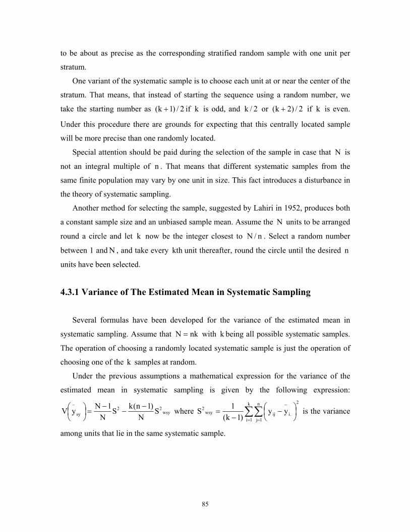
4.3.1 Variance of The Estimated Mean in Systematic Sampling

Several formulas have been developed for the variance of the estimated mean in

systematic sampling. Assume that nkN = with k being all possible systematic samples.

The operation of choosing a randomly located systematic sample is just the operation of

choosing one of the k samples at random.

Under the previous assumptions a mathematical expression for the variance of the

estimated mean in systematic sampling is given by the following expression:

wsy22

sy SN

)1n(kSN

1NyV −−

−=

−

where 2k

1i

n

1j.iijwsy

2 yy)1k(

1S ∑∑= =

−

−

−= is the variance

among units that lie in the same systematic sample.

86

An alternative form for the variance is given by the following expression.

[ ]w

2

sy )1n(1N

1Nn

SyV ρ−+

−

=

−

where wρ is the correlation coefficient between

pairs of units that belong to the same systematic sample and it is defined as

2ij

iuij

w

)Yy(E

YyYyE

−

−−

−

−

−

=ρ .

4.3.2 Stratified Systematic Sampling

There are cases where the systematic sampling can be combined with stratified

sampling. This is possible in the case that we choose to stratify the sample according to

some criteria and then draw a separate systematic sample within each stratum with

starting points independently determined. This method will be more precise than the

stratified random sampling if systematic sampling within strata is more precise than

simple random sampling within strata. If syhy−

is the mean of the systematic sample in

stratum h , the estimate of the population mean −

Y and its variance are given by

∑∑−−−−

== syh2

hstsysyhhstsy )y(Vw)Y(V ,ywY .

In practice the stratified systematic sampling is used in the labour force surveys in

Sweden and in Finland. More specifically, in these countries the sampling unit is the

individual. The population is stratified according to variables such as sex, region and

employment status and finally a systematic sample is drawn from each stratum.

4.4 Cluster Sampling

Clustering or cluster sampling denotes methods of selection in which the sampling

unit, the unit of selection contains more than one population element; hence the sampling

unit is a cluster of elements (individuals). This sample design can be applied either in one

or in more steps. If it is applied in one step, then in this single step, we select a sample of

87

primary units (clusters) and we take into account the whole amount of elements that each

primary unit contains. If it is applied in more than one step, after the selection of the

primary units, we sub-sample in order to select only some of the elements that each

primary unit contains.

There are two main reasons for the widespread application of cluster sampling.

Although the first intention is to use the elements as the sampling units, it was found in

many surveys that no reliable list of elements in the population is available. For example

in many countries there are no up-to date lists of people, houses or farms in large

geographic regions. However, a region can be divided into area units such as blocks in

the cities and segments of land. Even when a list of elements is available, economic

considerations may lead to the choice of a larger cluster unit. Generally, if we compare a

cluster sample with an element sample of the same size, we will find that in cluster

sampling (1) the cost per element is lower due to the lower cost of listing (2) the element

variance is higher and (3) the costs and problems of statistical analysis are higher.

Clustering should be preferred over individual selection when the lower cost per element

comprises for its two disadvantages.

In the following paragraphs we describe the cluster sampling in more than one stage

in the case that we have either equal primary units or unequal primary units. Also we

focus on the most frequently sample design where the multistage cluster design is

combined with the stratified sampling Finally, we describe cases derived from European

surveys where the multistage cluster sampling is applied.

4.4.1 Sub-Sampling With Units of Equal Size

In the majority of the sample surveys that are conducted in the European Union, a

sample design applied in one stage is not sufficient by itself. This happens because

sometimes it seems uneconomical to take into account every element of the primary unit

(cluster). This technique of taking the sample in more than one stage, is called sub-

sampling, since the primary unit is not measured completely but is sampled itself.

Another name due to Mahalanobis is two-stage sampling, because the sample is taken in

two steps. Consequently many Member States apply more complex sample designs such

88

as the multistage sampling. In the sequel the two and the three stage sampling designs are

described for the case that the primary units are of equal sizes and formulas for the

estimates and the variance of these estimates are obtained. The scope of this part is not to

fully enumerate all the possible ways of choosing a sample. This is impossible since

every Member State has a unique methodology. This part only intends to describe the

philosophy of how we obtain estimates when we deal with sampling in more than one

stage and the primary units are of equal size.

The principal advantage of two-stage sampling is that it is more flexible than one

stage sampling. When sub-units in the same unit agree very closely, considerations of

precision suggest a small value of sub-sample. On the other hand, it is sometimes almost

as cheap to measure the whole of a unit than to sub-sample it. This happens for example

when the unit is a household and a single respondent can give accurate data about all

members of the households.

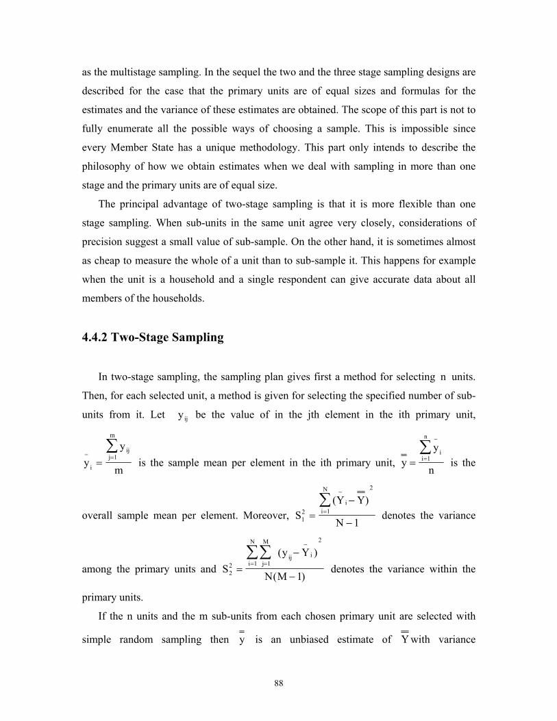
4.4.2 Two-Stage Sampling

In two-stage sampling, the sampling plan gives first a method for selecting n units.

Then, for each selected unit, a method is given for selecting the specified number of sub-

units from it. Let yij be the value of in the jth element in the ith primary unit,

yy

mi

ijj

m

− ==

∑1 is the sample mean per element in the ith primary unit, y

y

n

ii

n

=

−

=∑

1 is the

overall sample mean per element. Moreover, SY Y

N

ii

N

12 1

2

1=

−

−

−

=∑ ( )

denotes the variance

among the primary units and Sy Y

N Mj

M

ij ii

N

22 11

2

1=

−

−=

−

=∑∑ ( )

( ) denotes the variance within the

primary units.

If the n units and the m sub-units from each chosen primary unit are selected with

simple random sampling then y is an unbiased estimate of Y with variance

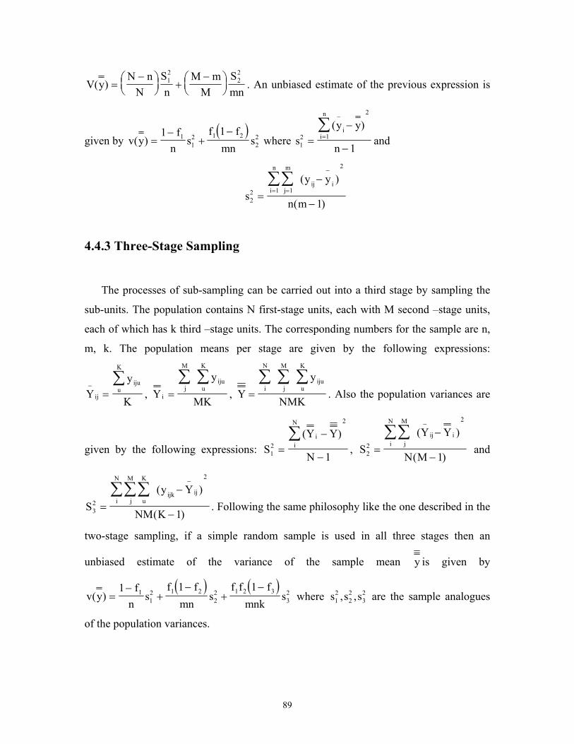
89

V yN n

NSn

M mM

Smn

( ) =−

+

−

12

22

. An unbiased estimate of the previous expression is

given by ( )

v yf

ns

f fmn

s( ) =−

+−1 11

12 1 2

22 where s

y y

n

ii

n

12 1

2

1=

−

−

−

=∑ ( )

and

sy y

n mj

m

ij ii

n

22 11

2

1=

−

−=

−

=∑∑ ( )

( )

4.4.3 Three-Stage Sampling

The processes of sub-sampling can be carried out into a third stage by sampling the

sub-units. The population contains N first-stage units, each with M second –stage units,

each of which has k third –stage units. The corresponding numbers for the sample are n,

m, k. The population means per stage are given by the following expressions:

Yy

Kij

ijuu

K

−=

∑, Y

y

MKij

M

ijuu

K

=∑ ∑

, Yy

NMKi

N

j

M

ijuu

K

=∑ ∑ ∑

. Also the population variances are

given by the following expressions: SY Y

N

ii

N

12

2

1=

−

−

∑ ( ), S

Y Y

N Mj

M

ij ii

N

22

2

1=

−

−

∑∑−

( )

( ) and

Sy Y

NM Ku

K

j

M

ijk iji

N

32

2

1=

−

−

∑∑∑−

( )

( ). Following the same philosophy like the one described in the

two-stage sampling, if a simple random sample is used in all three stages then an

unbiased estimate of the variance of the sample mean y is given by

( ) ( )v y

fn

sf f

mns

f f fmnk

s( ) =−

+−

+−1 1 11

12 1 2

22 1 2 3

32 where s s s1

222

32, , are the sample analogues

of the population variances.

90

4.4.4 Stratified Sampling of The Units in Two-Stage Sampling

Sub-sampling may be combined with any type of sampling of the primary units. The

sub-sampling itself may employ stratification or systematic sampling. Variance formulas

can be build up from the formulas of the simple methods.

Assume that the primary units in a two-stage sampling are obtained through

stratification. The hth stratum contains hN primary units, each with hM second stage

units. The corresponding sample units are hn and hm . The estimated population mean

per second stage unit is hh

h

hhh

hhhh

st yWMN

yMNy ∑∑

∑== where ∑= hhhhh MN/MNW is

the relative size of the stratum in terms of second-stage units and hy is the sample mean

in the stratum. The estimated population variance is given by

−+

−= ∑ 2

h2hh

h22h1

h

h12

hhst S

mnf1S

nf1W)y(V where hhh2hhh1 M/mf,N/nf == . An

unbiased sample estimate is

−+

−= ∑ 2

h2hh

h2h12h1

h

h12

hhst s

mn)f1(fs

nf1W)y(v where

( ) ( ))1m(n

yys and

1n

yys j

iiji2

2

n

i2

1 −

−=

−

−=

∑∑∑ express the variance among primary unit

means and the variance among sub-units within primary units respectively.

4.4.5 Sub-Sampling With Units of Unequal Size

In most clustered samples, we must deal with clusters of unequal sizes. Natural

clusters of both human and non-human populations contain unequal numbers of elements

e.g. dwellings in blocks or houses in villages Even a sample designed and initiated with

equal clusters may often end up with unequal clusters. Moreover, non-response is another

factor, which introduces inequalities into the final cluster results.

91

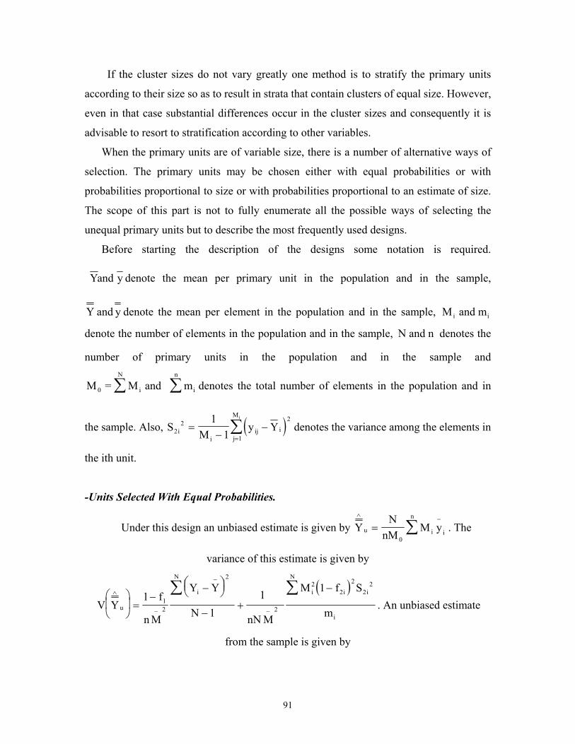
If the cluster sizes do not vary greatly one method is to stratify the primary units

according to their size so as to result in strata that contain clusters of equal size. However,

even in that case substantial differences occur in the cluster sizes and consequently it is

advisable to resort to stratification according to other variables.

When the primary units are of variable size, there is a number of alternative ways of

selection. The primary units may be chosen either with equal probabilities or with

probabilities proportional to size or with probabilities proportional to an estimate of size.

The scope of this part is not to fully enumerate all the possible ways of selecting the

unequal primary units but to describe the most frequently used designs.

Before starting the description of the designs some notation is required.

Yand y denote the mean per primary unit in the population and in the sample,

Y and y denote the mean per element in the population and in the sample, Mi and mi

denote the number of elements in the population and in the sample, N and n denotes the

number of primary units in the population and in the sample and

M0 = M and mi

N

i

n

∑ ∑ denotes the total number of elements in the population and in

the sample. Also, ( )SM

y Yii

ij ij

Mi

22

2

1

11

=−

−=∑ denotes the variance among the elements in

the ith unit.

-Units Selected With Equal Probabilities.

Under this design an unbiased estimate is given by YN

nMM yu i i

n∧−

= ∑0

. The

variance of this estimate is given by

( )V Y

f

n M

Y Y

N nN M

M f S

mu

i

N

i i i

N

i

∧

−

−

−

=

−−

−+

−∑ ∑11

1 112

2

2

22

2

22

. An unbiased estimate

from the sample is given by

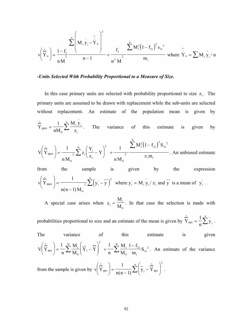
92

( )v Y

f

n M

M y Y

n

f

n M

M f s

mY M y nu

i i u

n

i i i

n

iu i i

∧

−

− −∧

−

−∧

−

=

−

−

−+

−=

∑∑

∑11

112

2

1

22

22

2

22

where /

-Units Selected With Probability Proportional to a Measure of Size.

In this case primary units are selected with probability proportional to size zi . The

primary units are assumed to be drawn with replacement while the sub-units are selected

without replacement. An estimate of the population mean is given by

YnM

M yzppesi i

i

n∧−

= ∑1

0. The variance of this estimate is given by

( )V Y

n Mz

Yz

Yn M

M f S

z mppes ii

i

N i i i

N

i i

∧

= −

+

−

∑∑1 1 1

0

2

2

0

2

22

2

22

. An unbiased estimate

from the sample is given by the expression

( )v Yn n M

y y M y z yppes i

n

i i i i

∧−

=

−− =∑

1

1 0

2

2

( )/' ' ' ' where y and is a mean of yi

' .

A special case arises when zi =MM

i

0. In that case the selection is made with

probabilities proportional to size and an estimate of the mean is given by Yn

ypps i

n∧−

= ∑1.

The variance of this estimate is given

V Yn

MM

Y Yn

MM

fm

Sppsi

i

Ni i

ii

N∧

= −

+

−∑ ∑1 1 1

0

2

0

22

2 . An estimate of the variance

from the sample is given by v Yn n

y Ypps i pps

n∧ ∧

=

−−

∑

11

2

( ).

93

-Units Selected With Probability Proportional to a Measure of Size - Ratio to Size

Estimate.

The selection of units with probability proportional to size appears highly efficient,

but the sampler possesses only estimates of the relative sizes zi . In this case an alternative

estimate for the mean in two-stage cluster sampling with unequal clusters is given by

YM y z

M zRppes

n

i i i

n

i i

∧

−

=∑

∑

/

/. The variance of this estimate is given by

V Yn

MM z

Y Yn

MM z

fm

SRppesi

ii

Ni

i

i

ii

N∧

= −

+

−∑ ∑1 1 12

02

2 2

02

22

2 . The estimate of the

variance is given by v Yn n M

Mz

y YRppesi

ii Rppes

n∧ ∧

=

−−

∑11 0

2

2

( ).

4.4.6 Stratified Sampling of The Units in Two-Stage Cluster Sampling

with Unequal Clusters

In the majority of applications the primary units are selected with stratified sampling.

If h denotes the stratum, M0h the total number of sub-units in stratum h and

M0 = ∑ M hh

L

0 the total number of sub-units in the population the estimated mean per sub-

unit is given by y W yMMst h h

h

Lh= =∑ , Wh

0

0. The variance of the estimate from the

sample is given by ( ) ( )v y W v yst h hh

L

= ∑ 2 . The variance formulas are obtained from the

previously referred formulas depending on the selection design that we have selected.

94

4.4.7 Application of Multistage Cluster Sampling in European Surveys

The multistage cluster sampling is perhaps the most frequently used sample design.

There are a number of advantages in using clustered, multistage sampling. By

concentrating the units to be enumerated, it reduces travel costs and other costs of data

collection. For the same reason, this sample design can improve the coverage,

supervision, control, follow up, and other aspects of determining the quality of the data

collected. The major disadvantage is the decrease in efficiency of the sample due to

clustering. The complexity of the design and the analysis are also increased.

In the household budget surveys, sample designs involve the selection of the samples

in multiple stages. Summing up the individual cases (Member States) we identify that the

most common practice is to use a two-stage sampling. First, a stratified sample of suitable

area units is selected, typically with probabilities proportional to size (PPS selection)

after stratification by geographical areas and other variables. The second stage consists of

the selection of households or addresses for inclusion in the survey. There are cases

where a three-stage is used. An example is Greece, where initially we have a two-area

stage (first some larger areas are selected as primary units, then one or more smaller areas

are selected from each primary unit) and a stage where households or addresses are

selected.

Multistage cluster sampling is used also in the European Community household

surveys. In the majority of cases a two-stage sampling is applied (selection of areas and

then selection of households within the selected areas). However, there are cases where a

single-stage cluster sample or element sample is used (Denmark, Luxembourg, Northern

Ireland).

In labour force surveys the sampling designs are similar to those previously

described. For example Belgium, Ireland and Spain use a two-stage stratified cluster

design and Greece follows a three stage stratified cluster design.

95

4.5 Post Stratification or Stratification After Selection

The motive for using stratification is based on the belief that responses of people may

vary with age, sex, occupation, education and similar factors none of which are available

for stratification at the individual level prior to sampling. However, censuses provide

information on all these variables at the aggregated level. If after selection of the sample

the individual units are cross-classified according to these factors then the known census

totals can be employed as measures of the population size to obtain estimates of the

population totals in each cell. The aggregate of these estimates yields an overall

population estimate and this procedure is known as post stratification or stratification

after selection. The one way post stratification is potentially more efficient than

stratification before selection, since after sampling, the stratification factor can be chosen

in different ways for different sets of variables in order to maximise the gains in

precision. The post stratification technique is particularly useful in multipurpose surveys

where stratification factors selected prior to sampling may be poorly correlated with large

numbers of secondary variables.

Assume that the population comprises N units which can be partitioned into H strata

of sizes .N,...,N,N H21 A variable Y takes values hiY h1,2,...Ni ,H,...,2,1h == . The

sample is of fixed size n which after selection falls into the strata according to the vector

∑ == nn ),n,...,n,n(n hH21 . The components of n are not known until the sample is

drawn. The sample mean and the sample variance in the hth stratum are

( )1n/)yY(s ,n/Yy h2

hhi2

hhhih −−==−−

∑∑ . The post-stratified estimator of −

Y is

given by ∑−

−

=

h

hh

estps

NyN

Y . We observe that each stratum mean is weighted by the

relative size of that stratum. Thus if a sample is badly balanced for some characteristic

the post - stratified estimator automatically corrects for this. This procedure is widely

used and its only obvious drawback is the lack of control over the sample allocation

which in extreme circumstances may lead to some hn being zero.

One would have thought at this point that since there is no disagreement about the

statistical analysis of stratified samples there would be no disagreement about the

96

analysis of post stratified samples. However, this is not the case and a clear divergence

can be found. Actually, there is no disagreement about the form of the post stratified

estimator assuming that the stratum sizes are known, but there is a disagreement

concerning the variance of the post stratified estimator and in particular the sampling

distribution to which it should be related.

There are two views on this problem. The first suggests a distribution conditional on

the vector n of the stratum sample sizes actually attained in the sample under study. The

second suggests the unconditional distribution determined by all possible sample sizes of

fixed size n . The form of the conditional variance is given by

h

2h

h h

h2

hestps

nS

Nn1

NNn/)Y(V ∑

−

=

−

which is the usual variance of stratified

samples. The unconditional variance is given by

( ) ( ) 2h

h

h22h

h

h11

h

1h

1h

2h

2h

estps SN

N1nSN

NNnNnESN

N)Y(V ∑∑∑

−+

−≅−

= −−−−−

−

where the approximation for ( )1hnE − is due to Stephan (1945)21. The question is which

variance (the conditional or the unconditional) should be used. Hansen et al. (1953) and

Des Raj (1972)22 are quite clear and advocate the use of the unconditional form with 2hS

estimated by 2hs . Cochran (1963) and Kish (1965) also advocate the use of the

unconditional variance for the post stratified estimate. On the other hand Yates (1960)

advocates the use of the conditional variance. This position is supported on the theoretical

grounds by Durbin (1969)23 who argues that the achieved sample size should be treated

as an ancillary statistic and hence the sample sizes should be made conditional on n . Cox

and Hinkley (1974)24 adopt also a similar position. A general rule that can be applied in

order to overcome this dilemma is the following. When comparing sampling strategies

before the sample is drawn the unconditional variance should be used whereas for

inferences after the sample is drawn the conditional variance is appropriate. This happens

21 see the Expected Value and Variance of the Reciprocal and Other Negative Powers of a Positive Bernoullian Variate. Annals of Mathematical Statistics., 16, 50-61. 22 see The Design of Sample Surveys. New York: McGraw-Hill. 23 see Inferential Aspects of the Randomness of Sample Size in Survey Sampling. New Developments in Survey Sampling. NewYork: Wiley. 24 see Theoretical Statistics by Cox and Hinkley. London: Chapman and Hall.

97

because after the sample is drawn we know the configuration of n and as a result we

know whether it is close to a proportional allocation or not.

Post stratification requires: (a) information on the proportions hW of the population

in the several strata and (b) information for classifying the sample cases into the same

strata. It must be stressed that the criteria of classification must be the same for (a) and

(b) and if they differ, the procedure is biased. As we have already said, post stratification

does not require, as proportionate selection does, every member of the population to be

classified and sorted into each stratum before selection. The question that is raised at this

point is when should post stratification be used instead of a proportionate selection.

Generally speaking some cases where post stratification is suggested are the following:

(1) When the stratifying variable is not available for classifying and sorting each

element.

(2) When the stratified variable although available, is not used. Perhaps at the time of

selection the sampler overlooked it or perhaps there were too many variables

available and he chose some others instead.

(3) Post stratification may be used on the subclasses even if a proportionate sample of the

entire population has been already selected. The effect of proportionate sampling

becomes lost on small subclasses; the sample sizes vary into strata and the variance of

the mean approaches that of the simple random sampling. By introducing the proper

weights, the number of subclass members in each stratum can restore most of the

gains of proportionate sampling.

The post stratification is a technique that can be applied to the simplest case of a

single stage design or in situations of more complex survey designs. Especially in the

case of multipurpose surveys the post stratification may be employed in such a way that

different sets of post strata variables estimate different variables. Concluding, this

technique can be viewed as a robust technique that offers protection against unfavorable

sample configurations and against non-response bias.

98

4.5.1 Post-Stratified Non-Response Adjustment

As we have already mentioned the post-stratification technique can offer protection

against non-response bias.

Assume that hiY is the characteristic to be studied for the ith unit in the hth sub-

population with hN,...,2,1i = and H,...,2,1h = . The post-stratified estimator treats the

sub-populations as strata employing the known { }hN and the number of responses { }hm

in each of the H groups. Expressing now the post-stratified estimator we obtain the

following expression ∑=

H

1h

~

h

h

estps

~Y

mN

Y .

The assumptions behind this estimator are the following: (1) We assume that within

each sub-population, the response mechanism is an independent Bernoulli sampling

process with common probability 0h >Φ of a response for each of the hn sampled units

and (2) the response mechanisms are independent from one sub-population to another.

4.6 Raking Ratio Adjustment.

The raking ratio adjustment was first proposed by Deming and Stephen25 as a way of

assuring consistency between complete count and sample data from the 1940 U.S. census

of population. Since then their procedure has been used for a variety of problems

including that of adjusting for non-response.

The raking ratio estimation is an iterative procedure for scaling sample data to known

from other sources marginal totals. One way to specify the raking algorithm is to set up a

series of constrained equations. Assume, a two-way table of weighted counts

( ){ }hkn n/N where H,...,2,1h = and K,...,2,1k = . Assume that the row { }.hN and

column { }k.N population marginal totals are known. Suppose further that we want to

obtain adjusted counts such that

25 see On a Least Square Adjustment of a Sampled Frequency Table When the Expected Marginal Totals Are Known. Annals of Mathematical Statistics 11: 427-444.

99

=

=

∑

∑

k.hk~H

1

.hhk

~K

1

NnnN

NnnN

To derive adjusted counts so that the previous expression hold, the raking algorithm

proceeds by proportionately scaling the cell values { }hkn so that each of the equations is

satisfied in turn. Each step begins with the results of the previous step, and the process is

terminated when all the equations are simultaneously satisfied to the closeness desired.

4.6.1 Raking Non-Response Adjustment.

The discussion of raking as a non-response adjustment technique requires the

following stipulations. Suppose, that we have L sub-populations )HKL( = with the

number of respondents in each sub-population being given by { }hkm where H,...,2,1h =

and K,...,2,1k = . Further, we assume that (1) within each sub-group the responses are

generated by an independent Bernoulli sampling process with common probability

0hk >Φ , (2) the response mechanisms are independent from one sub-population to

another, and (3) the { }hkΦ have a structure across subgroups such that

{ } khhkhk )1/(ln α+α=Φ−Φ . This means that the logarithm of the response probabilities

depends on constants { }hα and { }kα , or, in other words, that the response probabilities

are determined solely by the row or the column a unit fails and do not depend also the

particular cell. The first two of these conditions are the same as those postulated for the

post-stratification adjustment. The third condition is new and imposes a restriction that

we did not require earlier. On the other hand, we are not assuming here, as we did before,

that the 0mhk > . All that is needed is that the pattern of zeros among the hkm be such

that the algorithm converges.

100

The raking estimator in the case of non-response is then given by ∑∑−

=L

1

K

1

*

hkhk

~

r

~yNY

with hkk

~

h

~

hk

~mbaN = where

h

~a and

k

~b are the convergent adjustment factors

developed from the iterative use of the raking algorithm. 4.7 Sample Surveys in The European Union

In the following sections three sample surveys conducted in the European Union are

studied. The sample surveys that are analysed are the Labour Force survey, the European

Community Household Panel and the Household Budget survey.

Concerning these surveys an overview of the sampling designs and weighting

procedures is given. Furthermore, some attempts for harmonisation between the national

surveys are also described.

4.7.1 The Labour Force Survey (LFS) 4.7.1.1 The Objectives of The Labour Force Survey

The labour force survey is an inquire designed to obtain information on the labour

market and related issues by collecting data through administrative records and sample

surveys of households and enterprises. The labour force survey serves a number of

purposes. Firstly, it provides information on relevant labour market aspects across all

sections of economy. Moreover, it facilitates the interpretation of the information in a

wider population setting, since the information collected need not necessarily to be

confined to persons in the labour force but also to all people in the households covered.

Another advantage of the labour force survey is that it affords the opportunity to define

certain labour market characteristics not normally available from other statistical sources.

Due to the fact that definitions used to measure the entities are the same for each

country, the comparability between Member States is guaranteed for certain estimates.

This aspect is of considerable importance in the content of the European Union. There

are, however, some limitations connected with labour force survey. Cost considerations

101

place a constraint on the overall household sample size and the resultant sampling

variability limits the level of detail. Thus, while the labour force survey can be used to

compile estimates of employment across economic sectors, it cannot be expected to yield

reliable figures neither at a detailed level of regional disaggregation, nor for individual

small industrial or commercial sub-sectors. The sampling base on which such estimates

would depend would be to small and the degree of variability correspondingly high. For

the same reason, there is also a limit to what can be achieved with labour force survey in

monitoring trends over time.

4.7.1.2 The Development of The European Union Labour Force Survey

- Attempts For The Harmonisation of The Concepts

The first labour force survey was introduced on a monthly base in the United States in

1940. The movement towards the use of the labour force survey was somewhat slower in

Europe. Apart from the war another reason for this was the existence of alternative

sources of information which provided at least a partial insight into aspects of the labour

force. However, in time, as the need to take a more global view of the labour market

become apparent, European countries began to initiate labour force surveys. The first was

France in 1950. Germany initiated annual series of labour force survey in 1952 and

Sweden after experimentation a quarterly series in 1963. The first attempt to carry out a

labour force survey covering the European Community was made in 1960 with the six

original Member States.

The definitions used in the early surveys were necessarily somewhat imprecise, due

to the lack of internationally accepted terminology. This gap was filled in 1982 when the

thirteenth international conference of labour statisticians at Geneva, passed a resolution

concerning statistics of the economically active population, employment, unemployment

and underemployment, containing exact definitions of the various categories of the

population that the labour force survey indents to measure. The Member States agreed to

apply these recommendations in a new series of labour force surveys which would be

conducted annually.

102

A new series of surveys was introduced in 1992. The survey continued to be

conducted annually, but for the first time a criterion of statistical reliability at a regional

level was introduced. Furthermore, the list of variables and the questions related to the

job search were revised.

In the mid-1990´s a number of concurrent developments become apparent and new

statistical requirements emerged. More specifically there was a need for more recent and

more frequent data on employment trends for choosing employment policies. Also there

was need for annual estimates on average employment which take into account the

seasonal trends in employment. Moreover the measurement of annual volume of work

which takes account of the trends in part-time work was important. Last but not least, the

better knowledge of relations between earnings and certain forms of employment and

between household composition and participation was also of high importance. Thus,

after four years of negotiations with the Member States a new regulation that indents to

achieve the previously refereed targets was adopted.

4.7.1.3 Technical Features of The European Union Labour - Force

Survey

In an attempt to discriminate the responsibilities of each part that participates in the

design of the European Union labour force survey, we can say the following. The

technical aspects of the survey, are discussed by Eurostat and the representatives of the

respective national statistical institutes and the employment ministries. The national

statistical institutes are responsible for selecting the sample, preparing the questionnaires,

conducting the direct interviews to the households and forwarding the results to Eurostat

and especially to Unit E126. Eurostat, devises the programme for analysing the results and

is responsible for disseminating the information sent by the national statistical institutes.

The technical features of the EU labour force survey can be described by the

following components.

Field of survey: the survey is indenting to cover the whole of the resident population i.e.

all persons whose usual place of residence is in the territory of the Member States of the

103

European Union. Population leaving in collective houses is not included for technical and

methodological reasons. Consequently this comprises all persons living in the households

surveyed during the reference week, and all persons absent from the households for short

periods. People who have emigrated or moved to other households are not covered.

Reference period: the labour force characteristics refer to the situation of the sample unit

in a particular week.

Units of measurement: the main units of measurement are individuals and households.

Reliability of results: as in any sample survey, the results of labour force survey are also

affected by non-sampling errors (i.e. inability or unwillingness of the respondents to

provide correct answer or even answer at all). However, experience shows that at national

level the survey information provides sufficiently accurately estimates for the levels and

structures of the various aggregates into which the labour force is divided. Reliability of

the results is assured by the size of the samples and the sampling methods used in

addition to the thorough planning of the various survey operations.

Comparability over space: perfect comparability is difficult to be achieved.

Nevertheless, the degree of comparability is considerably high. This can be attributed to

the record of the same set of characteristics in each country, to a close correspondence

between the European list of questions and the national questions and to the use of the

same definitions and classifications for all countries.

Comparability over time: since 1983 improved comparability over time has been

achieved, mainly due to the greater stability of content and the higher frequency of the

surveys. However, there are some problems mainly due to modifications in the sample

designs and in the order of the questions or due to changes in the reference period and in

the adjustment procedures.

4.7.1.4 Sample and Weighting Procedures in Member States and Greece

Concerning The Labour - Force Survey

Concerning the labour force survey, the majority of the Member States use multistage

stratified clustered sample designs. Examples of countries that use such sample designs

26 Eurostat’s Unit E1 is responsible for the Labour Market characteristics.

104

are Belgium, Greece, Spain, Germany, Ireland, Italy, France and Netherlands. However

there are cases where element sample designs are used. This happens in Finland, Sweden

and Denmark. More specifically, Finland and Sweden use a stratified sample design with

systematic selection of the units while Denmark a stratified sample design with random

selection of the units.

As far as it concerns the weighting procedures, we have found that all countries

except Greece use the post-stratification method.

The labour force survey in Greece is a continuous one providing quarterly results.

The sample size is 30000 households which represents a rate of 0.87%. The survey base

for samplings is the census and the sampling unit is the household. Stratification is

carried out by administrative region and degree of urbanisation. Thus, each NUTS II

region constitutes the first stratification level. Within each NUTS II region, communes

and municipalities are stratified according to the department (NUTS III) region to which

they belong and to the population of the main town. A rotation system comprising six

waves is used. Each sampling unit is kept in the sample for six consecutive quarters.

No stratification is carried out a posteriori, while in the majority of the Member States

a posteriori stratification is carried out, and when a household fails to respond it is

replaced by the next household on the list.

4.7.2 The European Community Household Panel (ECHP)

4.7.2.1 Objectives of The European Community Household Panel

The European Community household panel is a standardised survey conducted in

Member States of the European Union under auspices of Eurostat i.e. Unit E227. (living

conditions and social protection). The survey involves annual interviewing of a

representative panel of households and individuals in each country, covering a wide

range of topics of living conditions. It was established in response to the increasing

demand for comparable information across the Member States on income, work and

27 Eurostat’s Unit E2 is responsible for the Living Conditions and the Social Protection.

105

employment, poverty and social exclusion, housing, health and many other diverse social

indicators concerning living conditions of private households and persons.

The ECHP forms a component of a co-ordinated system of household surveys aimed

at generating comparable social statistics at the European Union level. The two other

main and well-established components of the system are the Labour Force survey (LFS)

and the Household Budget survey (HBS). The ECHP has a central place in the

development of comparable social statistics in the EU and is designed to supplement

information generated by the LFS and the HBS surveys.

A major aim of the survey is to provide an up-to-date and comparable data source on

personal incomes. Information on incomes of households and persons is indispensable for

policy-makers at the national and European levels. The survey provides detailed

information at the individual and household levels on a variety of income sources: wage

income, rent subsidies, unemployment and sickness benefits, social assistant benefits,

occupational and private pensions. Hence the strength of the ECHP is its focus on the

income received from all sources by every member of the household.

4.7.2.2 Outline of The Design

Three characteristics make the ECHP a unique source of information. These are (a) its

multi-dimensional coverage of a range of topics simultaneously (b) a standardised

methodology and procedures yielding comparable information across countries and (c) a

longitudinal or panel design in which information on the same set of households and

persons is gathered in order to study changes over time at the micro level.

a) Multi-Dimensional Coverage

In each country, the survey begins with a nationally representative sample of a few

thousand households, interviewing around 60.000 households and 130.000 adults in the

European Union. Within each household of the sample, a listing of its members along

with their demographic characteristics is obtained. This is followed by a detailed

household interview. This covers information on migration status of the household,

106

tenure of accommodation, housing amenities and costs, possession of durable goods,

major sources of income and diverse indicators of the household’s financial situations.

Finally, all household member aged 16 and over are subject to a detailed personal

interview. Two major areas covered in considerable detail in the interview concern the

economic activity and the personal income. In addition, a wide range of other topics are

covered such as, the individual’s social relations and responsibilities, health, pension and

insurance, degree of satisfactions with various aspects of work and life, education and

training, and biographic information. Hence compared to other social surveys in the EU,

the ECHP has much broader and integrative character. It aims at providing comparable

and inter-related information on earnings and social protection, benefits employment and

working conditions, housing and family structures and social relations and attitudes.

b) Cross Sectional Comparability

The inter-relations that the ECHP aims to study can be analysed and compared across

countries. Comparability is achieved through a standardised design and common

technical and implementation procedures, with centralised support and co-ordination by

Eurostat. The ECHP has a number of features introduced to enhance comparability.

These are: (1) a common survey structure and procedures, (2) common standards for data

processing and statistical analysis including editing, variable construction, weighting,

imputation and variance computation, (3) common sampling requirements and standards,

(4) common frameworks of analysis through a collaborative network of researchers and

(5) common “blue-print” questionnaire which serve as the point of departure for all

national surveys.

c) Longitudinal or Panel Design

The unique feature of the ECHP is its panel design. Within each country, the original

sample of households and persons is followed over time at annual intervals. In this

manner, the sample reflect demographic changes in the population and continues to

107

remain representative of the population over time, except for losses due to sample

attrition and non-inclusion of the households.

In each wave, the sample data are edited, weighted and imputed as required to obtain

a representative picture of the study population. Similarly, across waves, the data are

linked, edited, imputed and weighted as required to construct micro-level database.

4.7.2.3 Sampling Aspects of The First Wave

• Sampling Frame Sampling Size and Allocation

The target population includes all the households throughout the national territory of

each country. The sampling frames used in the Member States included the population

register, master samples created from the most recent census of population and houses,

the postal address registers, and the electoral roll.

The sample size of each Member State was determined on the basis of various

theoretical considerations, practical considerations and the available budget. The total

community sample was slightly over 60.000 households and 130.000 persons aged 16

and over. Generally larger countries, because of their greater need for disaggregate results

and also greater capacity, received larger sample sizes. Mostly, the range is between

4.000 completed households and 7.800 completed personal interviews in the smaller

countries, and 7.500 households and 17.000 personal interviews in the larger ones.

Within each country, the sample was distributed proportionally across geographical

region, so as to maximise the precision of estimates at the national level. However, Italy

and Spain chose disproportionate allocations i.e. sampling smaller regions at higher rates

with a view to ensure a minimum sample size for each region of the country.

• Sample Design And Selection

All surveys in ECHP are based on probability sampling. Most of the surveys are

based on a two-stage sampling i.e. a selection of sample areas in the first stage, followed

by the selection of a small number of addresses or households at the second stage within

108

each selected area. However, there are cases where a single stage sample is drawn or

even a three-stage sample (i.e. large areas smaller clusters

addresses of households).

Diverse criteria are used for the stratification of area units before selection. The most

common criterion is the geographical region and/or urban-rural classification.

Stratification by population size and other social indicators is also used in some countries.

Within explicit strata, areas can be selected systematically or randomly.

4.7.2.4 Recommendations for Cross Sectional Weighting – A Step By

Step Procedure

• Design Weights

The design weights are introduced to compensate for differences in the probabilities

of selection into the sample. The weight given to each household is inversely proportional

to its probability of selection. With multi-stage sample design, the design weight refers to

the overall selection probabilities of the households. If ip is the overall sampling

probability of the household i , and in the number of households successfully

enumerated into the sample, the design weights are

=

∑∑

ii

i

ii p/n

np1w . The weights are

computed for all households selected, but the summation over in is confined to

households where the interview was completed.

In the majority of ECHP surveys, households have been selected with uniform

probabilities so that design weights are all the same. However, in a number of countries,

large variations in household selection probabilities exist.

• Non-Response Weight

In the ECHP surveys, non-response rates are generally high and vary across different

groups in the population. It is necessary therefore to weight the data for non-response.

109

These weights are introduced in order to reduce the effect of differences in unit responses

rates in different parts of the sample and are based on characteristics which are known for

responding as well for non-responding households. Weighting for non-response involves

the division of the sample into certain appropriate weighting classes, and the weighting of

the responding units inversely to their response rate. More specifically, the following

steps are involved:

-Division of the sample groups into groups of weighting classes, showing the number of

households that selected and the number of households that interviews were completed in

each class.

-Computation of the response rate for each category in the classification.

-Assignation of a uniform weight to all households in a category, in inverse proportion to

the response rate in this category.

-Normalisation the weights.

Basically, the response rate is computed as the ratio of the number of households

interviewed to the number of households selected in the weighting class. In addition, if

the households within a class have different design weights, then the response rate is

more appropriately computed as the ratio of the weighted number of households

interviewed to the weighted number of households selected.

In cases where additional information is available, the sample may be classified in

several ways, for instance by main geographical and stratification variables, or by other

characteristics of areas. Moreover when additional information is available for both

responding and non-responding households, the sample may be classified by tenure of

accommodation, by household size or type, and by other social -economic characteristics.

For each category in the classifications, the numbers of the households selected and the

number interviewed are obtained, and the response rates computed. By considering the

marginal distributions by each of these classification variables, a generalised raking

procedure can be used to control for them simultaneously. This means that the sample

data are weighted such that, after weighting, the marginal distribution of the interviewed

households agrees with the corresponding distribution of the household originally

selected into the sample.

110

• Weights Correcting The Distribution of Households

The third step in the weighting procedure has the purpose of adjusting the distribution

of households by various characteristics, so as to make the sample distribution agree with

the same from some more reliable external sources. The distribution in various categories

may involve numbers of households and/or aggregates of some variables measured on

each household.

The basic requirement is that the characteristics used for matching the sample

distribution to the external control distribution be the same in two sources, i.e. defined

and measured in exactly the same way. In most cases, the best available source of

information for this purpose is the labour force Survey or some other similarly large

survey.

In most situations it is not sufficient to consider the distribution by only a single

characteristic. It is desirable to control all important characteristics simultaneously. This

can result in too many controls to be applied, and consequently in small adjustment cells

and large variations in the resulting weights. Hence the procedure used in ECHP is to

control for a number of marginal distributions simultaneously, rather than to consider a

detailed classification. In order to achieve this, a generalised raking technique is used.

• Weights Correcting The Distribution of Persons

The next step in the ECHP weighting procedure involves the adjustment of the

household-level weights so as to make the distribution according to certain characteristics

covered in the sample agree with the same from some more reliable external source.

More specifically, this step controls the distribution of persons (with completed

interview) according to external information. The most important controls that are

applied in the ECHP are by age (normally in 5-year groups) and sex.

111

• Final weights

At the end of the weighting procedure, each household receives a weight which, is the

product of the weights assigned sequentially to it at the four previously described steps.

Any extreme weights are trimmed so as to avoid large inflation in variances. Finally, after

each step, the weights are normalised.

4.7.2.5 Second and Subsequent Waves of The ECHP

As we have already mentioned, the unique feature of the ECHP is its panel design.

Within each country, the original sample of households and persons is followed over time

at annual intervals. In this manner, the sample reflect demographic changes in the

population and continues to remain representative of the population over time.

The initial (wave1) sample consists of a probability sample of households in each

country. At any subsequent wave, the eligible population consists of the sample persons

i.e. (1) all initial (wave1) residents who are still alive and eligible for the ECHP, and (2)

children born subsequent to wave1, and those that become over 16 years old and as result

are eligible for interview. Newly formed households are added, resulting from the

movement of sample members since the last wave.

4.7.2.6 Longitudinal Weighting

Eurostat has recommended the following for longitudinal weighting. The starting

point for the weighting of panel data is provided by the initial weights of households and

persons enumerated in wave 1. These initial weights are adjusted to reflect main changes

in the study population and evolution of the sample over time.

More specifically we start with the initial weights )1(k,i

)1(i uu = . These refer to the weights

at 1t = for household i and for person k in hat household. Initial weights are computed

taking into account the selection probabilities of households in wave 1, the response rates

in wave 1, external information on the distribution of households, and external

112

information on the distribution of persons. These initial weights are defined for all

households interviewed and for all initial sample persons.

At each wave t, the basic weight )t(k,iu is obtained by adjusting the basic weight of the

previous wave )1t(k,iu − . This adjustment is made by using an adjustment factor f that

depends on changes in the population and the samples between waves t-1 and

t : )t1t(k,i

)1t(k,i

)t(k,i fuu ⇒−−= . The following adjustments are involved: (1) Adjustments for non-

response. Weights for wave t-1 are multiplied by a factor inversely proportional to the

person’s propensity to respond at wave t after having responded to wave t-1. (2) At each

wave the weights may be also adjusted for consistency with external information on the

distribution of the population. (3) Large variations in the weights is avoided by

constrained the adjustment factor within practical limits. (4) Children born between t-1

and t are given appropriate weights determined by the basic weights of their parents.

Sample persons from wave t-1 no longer alive are excluded from the survey while all

non-sample persons have a zero basic weight.

4.7.3 The Household Budget Survey (HBS)

4.7.3.1 The Objectives of The Household Budget Survey

The household budget surveys are sample surveys carried out in the Member States of

the European Union. The information collected via these surveys covers a wide variety of

items concerning consumption expenditure, income of private households, savings and

indebtedness, and other household characteristics.

The narrow purpose of the conducting household budget surveys is to obtain the

weights that are used for the construction of the consumer price indices and the cost of

living indices. The purpose of conducting an HBS in a more broad sense is to give a

picture of living conditions of private households in a defined area and time. In this

sense, the aim of the survey is to give a precise picture of the household’s total

consumption broken down in sufficient detail as a function of household characteristics

such as income, social and economic characteristics, size and composition, degree of

113

urbanisation, and region. The surveys also provide information about the living and

expenditure levels.

The use of the household budget surveys reflects their multipurpose character. The

use of the household budget surveys for constructing consumer price indices is being

reviewed in connection with establishing harmonised indices at the European Union

level. The surveys are also used as an input for building the national accounts for the

purpose of measuring household final consumption at an aggregate level. Furthermore,

the survey information is used widely as the basis for studies of living conditions and

nutrition patterns of private households and for analyses of poverty.

4.7.3.2 Attempts for The Harmonisation of The Concepts

Despite the common focus of the surveys on the study of the patterns of consumption

of private households, the national household budget surveys present a diversity of

structures and designs as well as differences in the topics covered. In order to reduce this

diversity Eurostat gives specific recommendations on many technical issues.

Harmonisation attempts of this type are: (1) the emphasis that is given on defining a

common approach to measure the consumption expenditure, and the income of the

households, (2) the agreement for the use of a common set of variables and (3) the

agreement for the use of a harmonised nomenclature regarding consumption.

Eurostat is committed in assisting Member States, as well as other interested

countries, for the improvement of their survey methods through the provision of

guidelines and direct technical support. Generally, Eurostat does not emphasise the use of

same questions or survey structure. The major importance is put into the use of

harmonising concepts and definitions. There are two reasons for this. Firstly it could be

argued that the adoption of certain definitions and concepts is not specifically based on

national circumstances but has a more universal character and secondly the use of certain

concepts and definitions can be justified by the nature of the survey. Examples of

concepts that Eurostat seeks to harmonise are the consumption expenditure and the

income of the households.

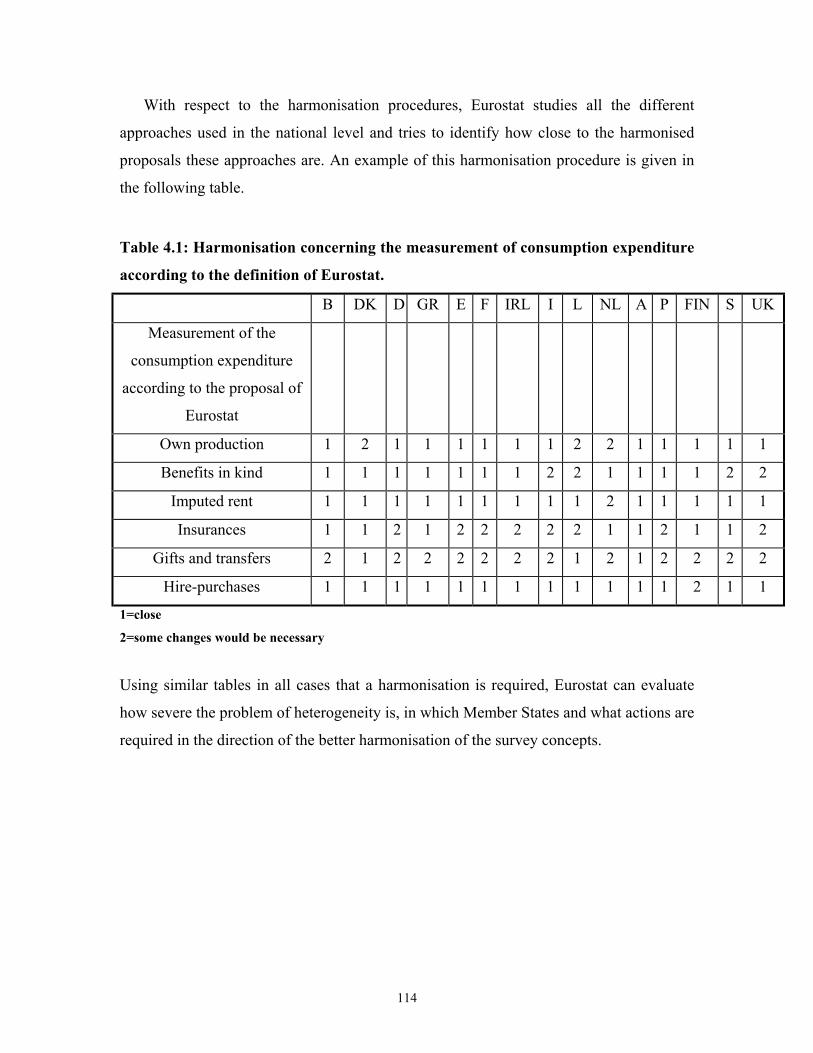
114

With respect to the harmonisation procedures, Eurostat studies all the different

approaches used in the national level and tries to identify how close to the harmonised

proposals these approaches are. An example of this harmonisation procedure is given in

the following table.

Table 4.1: Harmonisation concerning the measurement of consumption expenditure

according to the definition of Eurostat.

B DK D GR E F IRL I L NL A P FIN S UK

Measurement of the

consumption expenditure

according to the proposal of

Eurostat

Own production 1 2 1 1 1 1 1 1 2 2 1 1 1 1 1

Benefits in kind 1 1 1 1 1 1 1 2 2 1 1 1 1 2 2

Imputed rent 1 1 1 1 1 1 1 1 1 2 1 1 1 1 1

Insurances 1 1 2 1 2 2 2 2 2 1 1 2 1 1 2

Gifts and transfers 2 1 2 2 2 2 2 2 1 2 1 2 2 2 2

Hire-purchases 1 1 1 1 1 1 1 1 1 1 1 1 2 1 1

1=close

2=some changes would be necessary

Using similar tables in all cases that a harmonisation is required, Eurostat can evaluate

how severe the problem of heterogeneity is, in which Member States and what actions are

required in the direction of the better harmonisation of the survey concepts.

115

4.7.3.3 Sampling Aspects of The Household Budget Survey

All household budget surveys are confined to the population residing in private

households. As to the geographical coverage, most of the surveys cover the entire

population residing in private households in the national territory.

A variety of sampling frames exists for obtaining the sample for the household budget

survey: (1) Obtain the sample from households participating in another survey. There are

a number of advantages in selecting the sample as a sub-sample of some larger survey.

Firstly, more efficient stratification can be made and weighting for non-response is easier

by using information on non-respondents characteristics available from an earlier survey.

(2) Registers can provide up-to date lists of households or individuals, with many

relevant characteristics useful for stratification and efficient selection of the sample. (3)

Another common arrangement is to obtain a sample area of units from a suitable source

such as the population census or a master sample of areas. A master sample is a large

sample drawn for the purpose of common use in different surveys. It may be for example

a large sample of addresses from which samples for a particularly survey can be drawn

directly.

The range of the sample size varies from around 2000 in the Netherlands to 50000 in

Germany.

Probability sampling is used in the majority of the household budget surveys. Most

sample designs involve the selection of the sample in multiple stages. There are a number

of advantages in using multistage sampling. By concentrating the units to be enumerated,

the travel costs and other costs of data collection are reduced. For the same reason, it can

improve the coverage, supervision, control, follow up and other aspects determining the

response rates and the quality of the data collected. The major disadvantage is the

complexity of design and analysis. The most common practice is the use of a two-stage

design. First, a stratified sample of suitable area units is selected, typically with

probabilities proportional to size after stratification by region, social-economic status of

the reference person and household type or size. The second stage consists of the

selection, within each sample area, of households and addresses for inclusion in the

survey. However, there are cases where a three- stage sampling is performed. This design

116

involves a two area stages: first some larger areas such as localities are selected as the

primary sampling units; then one or more smaller areas are selected from the primary

sampling units and lastly, the household or addresses are selected.

In most cases the entire population is sampled uniformly and the sample is distributed

proportionately across different areas and population groups in the country. However, in

some surveys, population groups of special interest such as farmers or poorer households

are over-sampled.

4.7.3.4 Recommendations Concerning the Weighting Procedures

The need to weight data from the household budget survey is generally recognised.

Two types of weighting procedures are proposed. (1) Spatial weighting and (2) temporal

weighting.

The spatial weighting aims at improving the quality of the sample in relation to the

size, distribution and characteristics of the population, selection probabilities and survey

non-response. The procedure recommended by Eurostat is a multi-stage one similar to the

one described for the ECHP survey. Firstly, weights inversely proportional to the

probability of selection are calculated, next weights that take into account the non-

response are introduced and finally weights correcting for the distribution of households

are computed. The final weights are worked out as the product of the weights of the

previous stages.

The temporal weighting of the data stems from the fact that the household

observation period is often different from the reference period.

4.7.3.5 Procedures Followed in Greece Concerning the Household

Budget Survey

The household budget survey in Greece serves the following scopes: i.e. of revising

the Consumer Price Index, of estimating the total private consumption, of investigating

changes in the standard of living of households and finally of investigating the link

between household purchases and income.

117

The sampling method applied for this survey is the multistage stratified one. The

primary stratification criterion was the degree of urbanisation of the municipalities and

the communes in Greece. This criterion was used to create 11 main strata. In the first 6

major strata a two-stage sampling was employed while in the remaining strata a three-

stage sampling.

4.8 Concluding Remarks

The complex feature of this domain is the multivariate character of the surveys that

are being conducted in each Member State. Due to this complexity we have chosen to

describe two aspects of the surveys i.e. the sample designs and the weighting procedures.

In other words, we have tried to identify the most frequently used sample designs and

weighting procedures.

With respect to the sample designs we have found that generally the Member States

are in favour of clustered samples. More specifically, the Member States usually use

multistage stratified cluster samples with probability proportional to size or with uniform

probability selection for the primary units. However, there are cases where one-stage

element samples are used. These designs involve stratified samples with random or

systematic selection of the units within each stratum.

As far as it concerns the weighting procedures, we have found that the most

frequently used are the post-stratification and the raking ratio adjustment procedures.

Furthermore, in this chapter we have used the three surveys in order to investigate the

progress that has been made in the domain of the over space harmonisation of the

concepts and of the measurement procedures. Eurostat studies the different aspects of the

surveys that are being conducted in the Member State level in order to identify cases

where more harmonisation is required and to be able to make proposals for such a

harmonisation.

For the European household panel survey and for the household budget survey

Eurostat proposes a step by step cross sectional and a longitudinal weighting procedure.

This proposal aims at achieving harmonised weighting procedures. Another example of

harmonisation but in the sense of measuring common concepts is given for the labour

118

force survey. For this survey, the thirteenth international conference of labour

statisticians at Geneva, passed a resolution concerning statistics of the economically

active population, employment, unemployment and underemployment and generally

containing exact definitions of the various categories of the population that the labour

force survey indents to measure. The Member States agreed to apply these

recommendations in a new series of labour force surveys that would be conducted

annually. Similar harmonised targets are secured by the cross-sectional comparability

character of the European Community household panel. This character assumes the use

of common survey structures, of common standards for data processing and statistical

analysis and of common sampling requirements. Finally, harmonisation attempts of the

same type have been made also for the household budget survey. These attempts involve

the adoption of common definitions for the consumption expenditures and the income of

the households and for the use of a common set of variables.