chapter 3 water flow in pipes - islamic university of...

Water Flow in Pipes

The Islamic University of Gaza

Faculty of Engineering

Civil Engineering Department

Hydraulics - ECIV 3322

Chapter 3

2

3.1 Description of A Pipe Flow

• Water pipes in our homes and the distribution

system

• Pipes carry hydraulic fluid to various components

of vehicles and machines

• Natural systems of “pipes” that carry blood

throughout our body and air into and out of our

lungs.

5

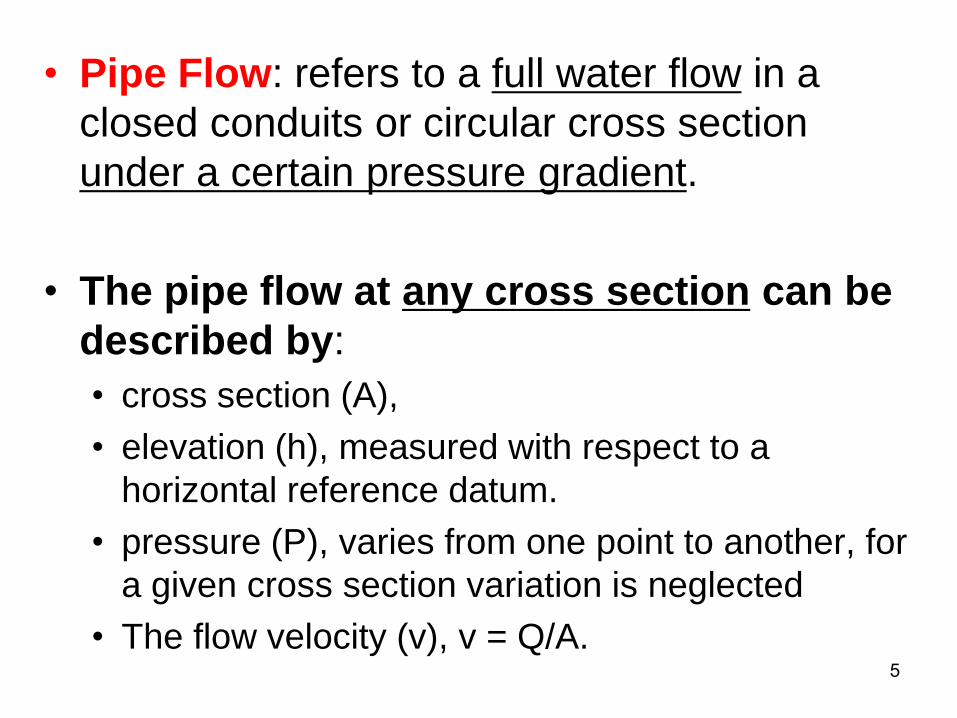
• Pipe Flow: refers to a full water flow in a

closed conduits or circular cross section

under a certain pressure gradient.

• The pipe flow at any cross section can be

described by:

• cross section (A),

• elevation (h), measured with respect to a

horizontal reference datum.

• pressure (P), varies from one point to another, for

a given cross section variation is neglected

• The flow velocity (v), v = Q/A.

6

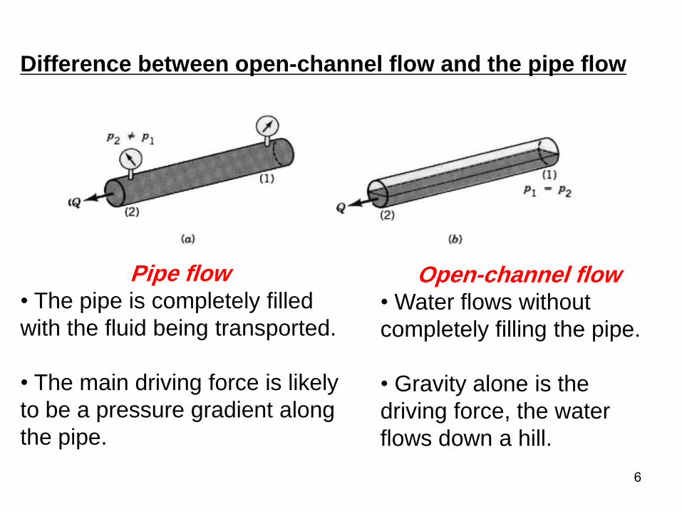
Difference between open-channel flow and the pipe flow

Pipe flow • The pipe is completely filled

with the fluid being transported.

• The main driving force is likely

to be a pressure gradient along

the pipe.

Open-channel flow • Water flows without

completely filling the pipe.

• Gravity alone is the

driving force, the water

flows down a hill.

7

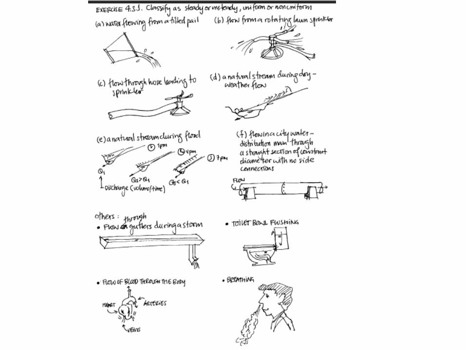
Types of Flow

Steady and unsteady flow Steady flow: conditions at any point remain constant,

but may differ from point to point. Velocities do not

change with time.

0ooo ,z,yx

tv

0ooo ,z,yx

tv

Unsteady flow: velocities change with time.

Based on time criterion

8

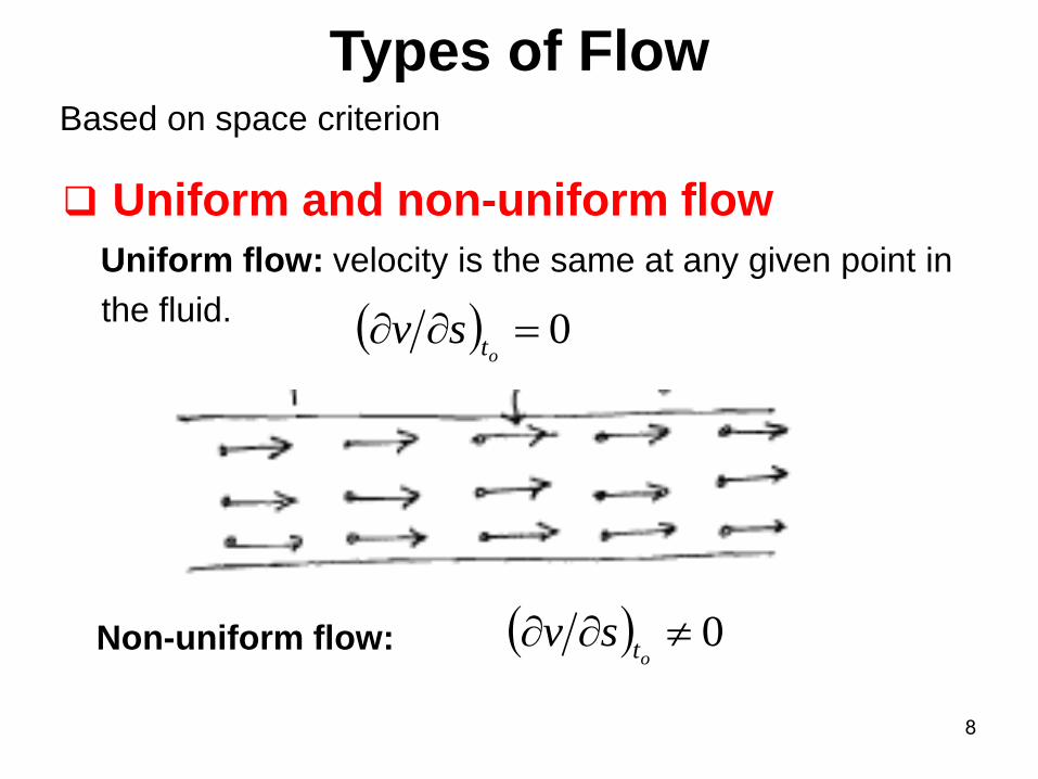
Uniform and non-uniform flow

Uniform flow: velocity is the same at any given point in

the fluid.

0

otsv

Non-uniform flow: 0ot

sv

Types of Flow Based on space criterion

9

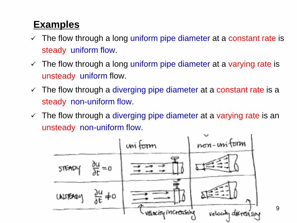
Examples

The flow through a long uniform pipe diameter at a constant rate is

steady uniform flow.

The flow through a long uniform pipe diameter at a varying rate is

unsteady uniform flow.

The flow through a diverging pipe diameter at a constant rate is a

steady non-uniform flow.

The flow through a diverging pipe diameter at a varying rate is an

unsteady non-uniform flow.

11

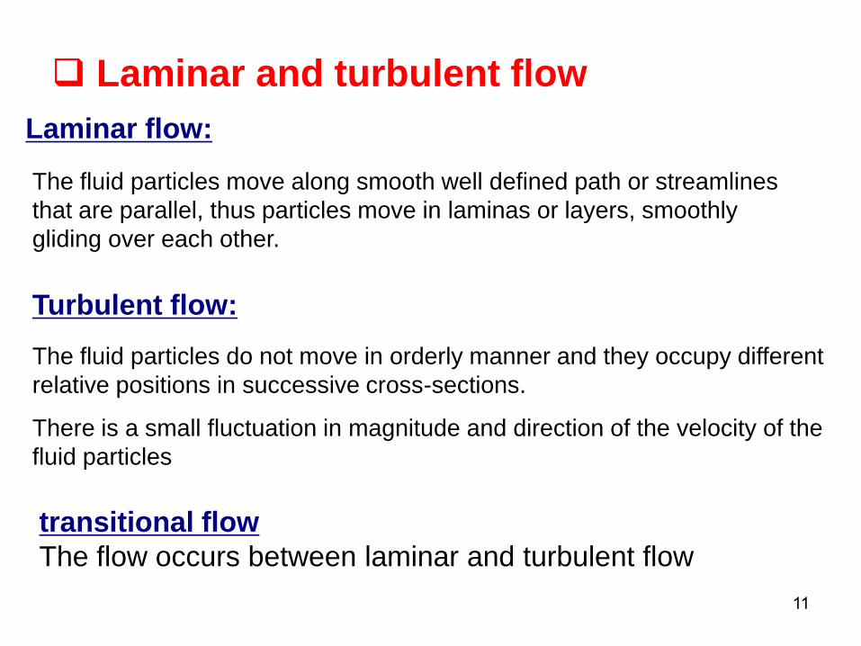
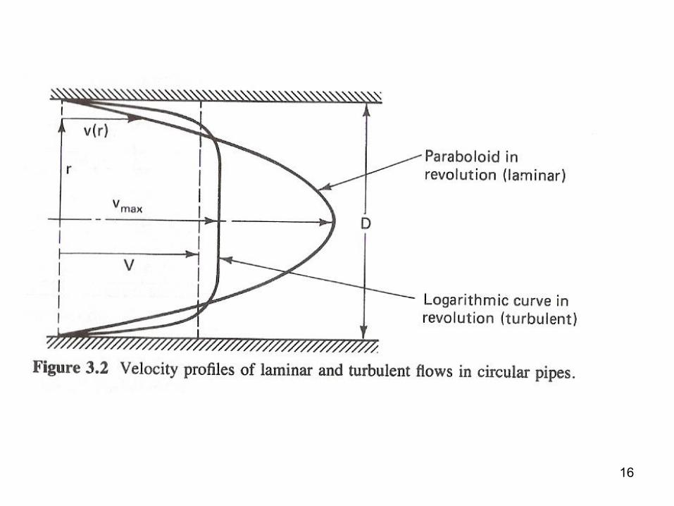
Laminar and turbulent flow

Laminar flow:

Turbulent flow:

The fluid particles move along smooth well defined path or streamlines

that are parallel, thus particles move in laminas or layers, smoothly

gliding over each other.

The fluid particles do not move in orderly manner and they occupy different

relative positions in successive cross-sections. There is a small fluctuation in magnitude and direction of the velocity of the

fluid particles

transitional flow

The flow occurs between laminar and turbulent flow

12

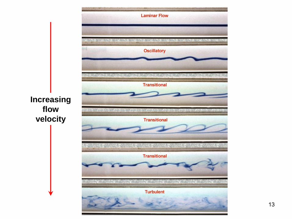
3.2 Reynolds Experiment Reynolds performed a very carefully prepared pipe flow

experiment.

13

Increasing

flow

velocity

14

Reynolds Experiment

• Reynold found that transition from laminar to turbulent

flow in a pipe depends not only on the velocity, but also

on the pipe diameter and the viscosity of the fluid.

• This relationship between these variables is commonly

known as Reynolds number (NR)

ForcesViscous

ForcesInertialVDVDNR

It can be shown that the Reynolds number is a measure of

the ratio of the inertial forces to the viscous forces in the

flow

FI ma AFV

15

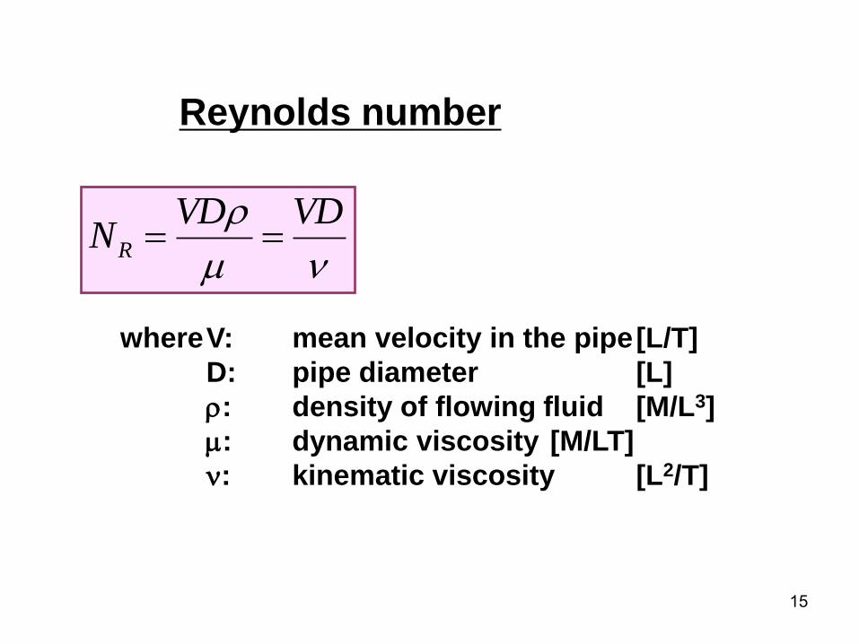
Reynolds number

VDVDNR

where V: mean velocity in the pipe [L/T]

D: pipe diameter [L]

: density of flowing fluid [M/L3]

: dynamic viscosity [M/LT]

: kinematic viscosity [L2/T]

17

Flow laminar when NR < Critical NR

Flow turbulent when NR > Critical NR

It has been found by many experiments that for flows in

circular pipes, the critical Reynolds number is about 2000

The transition from laminar to turbulent flow does not always

happened at NR = 2000 but varies due to experiments

conditions….….this known as transitional range

18

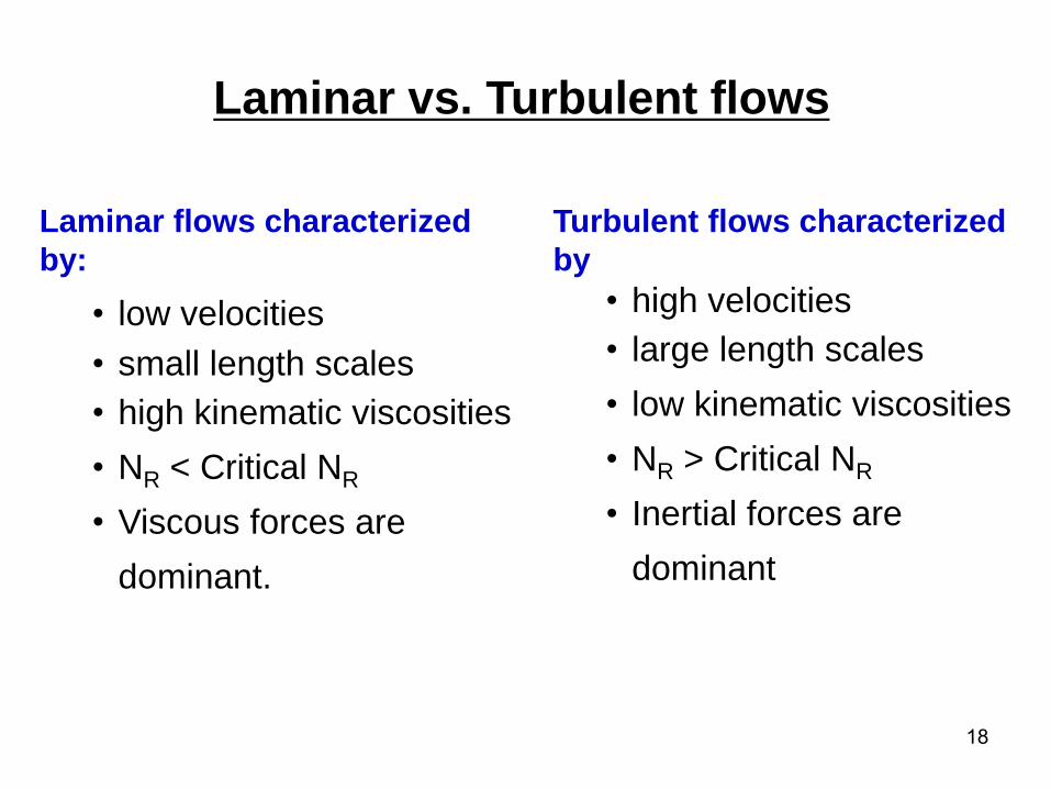
Laminar flows characterized

by:

• low velocities

• small length scales

• high kinematic viscosities

• NR < Critical NR

• Viscous forces are

dominant.

Turbulent flows characterized

by

• high velocities

• large length scales

• low kinematic viscosities

• NR > Critical NR

• Inertial forces are

dominant

Laminar vs. Turbulent flows

19

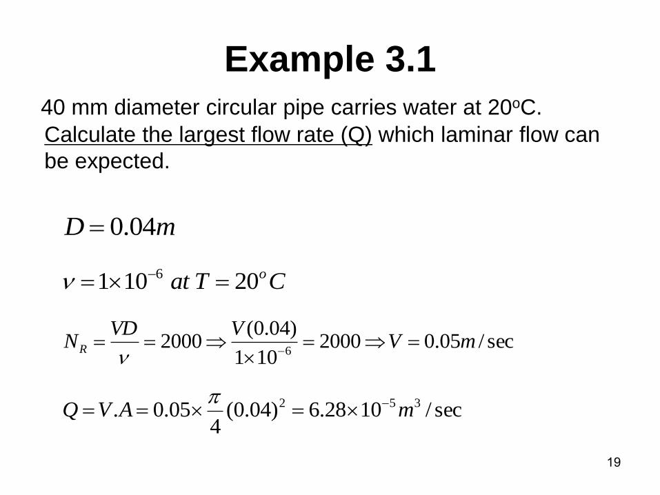
Example 3.1

40 mm diameter circular pipe carries water at 20oC.

Calculate the largest flow rate (Q) which laminar flow can

be expected.

mD 04.0

CTat o20101 6

sec/1028.6)04.0(4

05.0. 352 mAVQ

sec/05.02000101

)04.0(2000

6mV

VVDNR

20

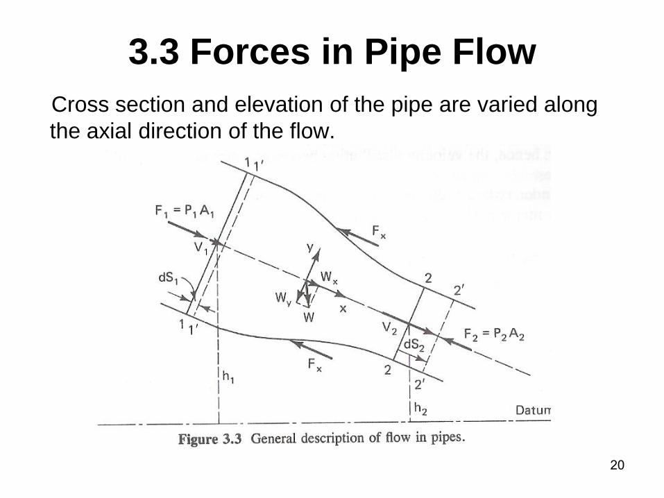
3.3 Forces in Pipe Flow

Cross section and elevation of the pipe are varied along

the axial direction of the flow.

21

)(.. '22'11 massfluidfluxmassdVoldVol

Conservation law of mass

Mass enters the

control volume

Mass leaves the

control volume

QVAVAdt

dSA

dt

dSA

dt

dVol

dt

dVol

.......

..

22112

21

1

'22'11

QVAVA 2211 ..

For Incompressible and Steady flows:

Continuity equation for

Incompressible Steady flow

22

Apply Newton’s Second Law:

t

VMVM

dt

VdMaMF

12

xxx WFAPAPF 2211

)(.

)(.

)(.

.

12

12

12

zzz

yyy

xxx

VVQF

VVQF

VVQF

rateflowmassQtMbut

Fx is the axial direction force exerted on the control volume

by the wall of the pipe.

)(. 12

VVQF

Conservation of

moment equation

23

dA= 40 mm, dB= 20 mm, PA= 500,000 N/m2, Q=0.01m3/sec.

Determine the reaction force at the hinge.

Example 3.2

24

3.4 Energy Head in Pipe Flow

Water flow in pipes may contain energy in three

basic forms:

1- Kinetic energy,

2- potential energy,

3- pressure energy.

25

Consider the control volume:

• In time interval dt:

- Water particles at sec.1-1 move to sec. 1`-1` with velocity V1.

- Water particles at sec.2-2 move to sec. 2`-2` with velocity V2.

• To satisfy continuity equation:

dtVAPdsAP ..... 111111

• The work done by the pressure force

dtVAdtVA .... 2211

dtVAPdsAP ..... 222222

-ve sign because P2 is in the opposite direction to distance traveled ds2

……. on section 1-1

……. on section 2-2

26

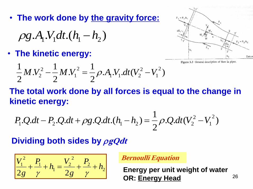
• The work done by the gravity force:

).(.. 2111 hhdtVAg

)(...2

1.

2

1.

2

1 2

1

2

211

2

1

2

2 VVdtVAVMVM

)(..2

1).(......

2

1

2

22121 VVdtQhhdtQgdtQPdtQP

• The kinetic energy:

The total work done by all forces is equal to the change in

kinetic energy:

Dividing both sides by gQdt

22

2

21

1

2

1

22h

P

g

Vh

P

g

V

Bernoulli Equation

Energy per unit weight of water

OR: Energy Head

27

Energy head and Head loss in pipe flow

28

11

2

11

2h

P

g

VH

22

2

22

2h

P

g

VH

Kinetic

head

Elevation

head

Pressure

head

Energy

head = + +

LhhP

g

Vh

P

g

V 2

2

2

21

1

2

1

22

Notice that:

• In reality, certain amount of energy loss (hL) occurs when the

water mass flow from one section to another.

• The energy relationship between two sections can be written

as:

29

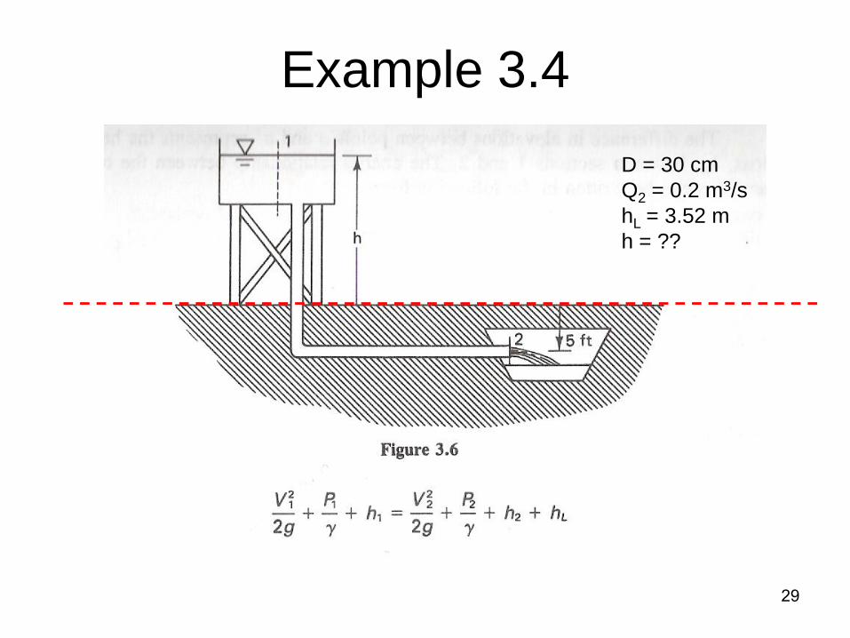
Example 3.4

D = 30 cm

Q2 = 0.2 m3/s

hL = 3.52 m

h = ??

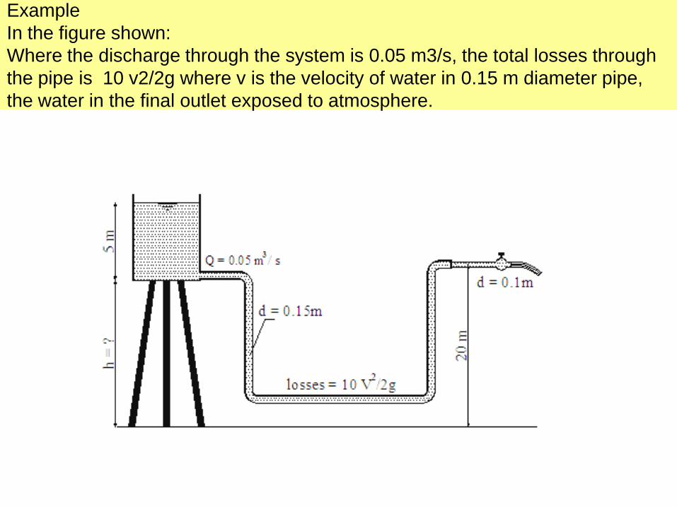
Example

In the figure shown:

Where the discharge through the system is 0.05 m3/s, the total losses through

the pipe is 10 v2/2g where v is the velocity of water in 0.15 m diameter pipe,

the water in the final outlet exposed to atmosphere.

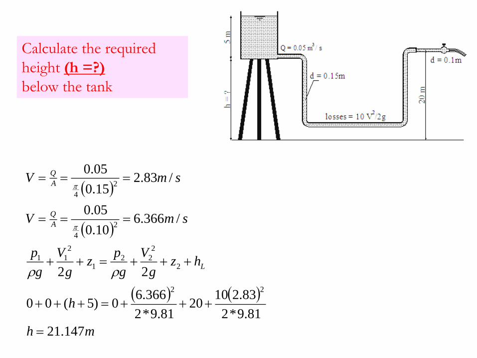
Calculate the required

height (h =?)

below the tank

mh

h

hzg

V

g

pz

g

V

g

p

smV

smV

L

A

Q

A

Q

147.21

81.9*2

83.21020

81.9*2

366.60)5(00

22

/366.610.0

05.0

/83.215.0

05.0

22

2

2

221

2

11

2

4

2

4

Without calculation sketch the (E.G.L) and (H.G.L)

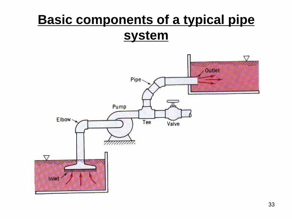
33

Basic components of a typical pipe

system

34

Calculation of Head (Energy) Losses:

In General: When a fluid is flowing through a pipe, the fluid experiences some

resistance due to which some of energy (head) of fluid is lost.

Energy Losses

(Head losses)

Major Losses Minor losses

loss of head due to pipe

friction and to viscous

dissipation in flowing

water

Loss due to the change of

the velocity of the flowing

fluid in the magnitude or in

direction as it moves

through fitting like Valves,

Tees, Bends and Reducers.

3.5 Losses of Head due to Friction

• Energy loss through friction in the length of pipeline is commonly

termed the major loss hf

• This is the loss of head due to pipe friction and to the viscous

dissipation in flowing water.

• Several studies have been found the resistance to flow in a pipe is:

- Independent of pressure under which the water flows

- Linearly proportional to the pipe length, L

- Inversely proportional to some water power of the pipe diameter D

- Proportional to some power of the mean velocity, V

- Related to the roughness of the pipe, if the flow is turbulent

36

Major losses formulas

• Several formulas have been developed in the past. Some of these formulas have faithfully been used in various hydraulic engineering practices.

1. Darcy-Weisbach formula

2. The Hazen -Williams Formula

3. The Manning Formula

4. The Chezy Formula

5. The Strickler Formula

37

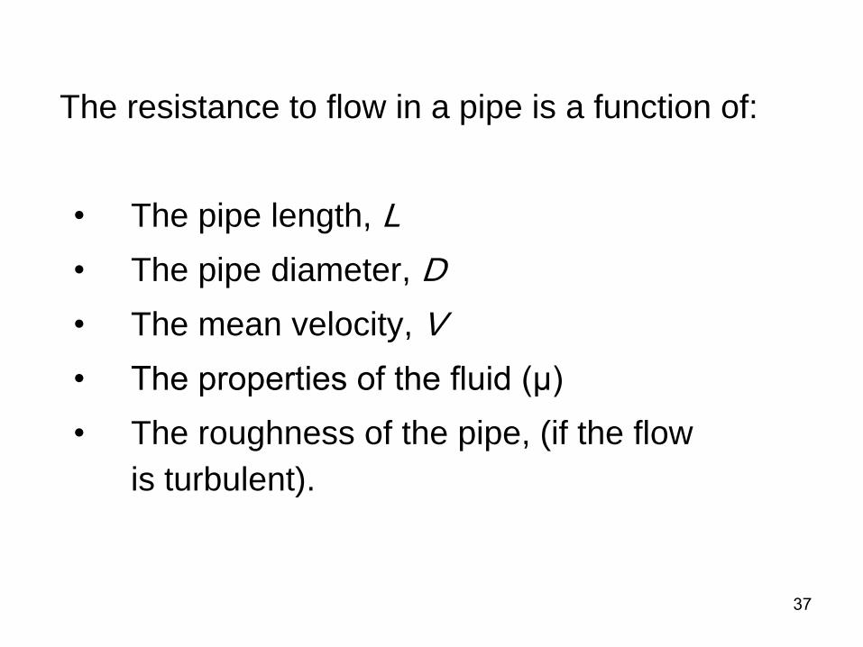
The resistance to flow in a pipe is a function of:

• The pipe length, L

• The pipe diameter, D

• The mean velocity, V

• The properties of the fluid (µ)

• The roughness of the pipe, (if the flow

is turbulent).

Darcy-Weisbach Equation

25

22

8

2

Dg

QLf

g

V

D

LfhL

Where:

f is the friction factor

L is pipe length

D is pipe diameter

Q is the flow rate

hL is the loss due to friction

It is conveniently expressed in terms of velocity (kinetic) head in the pipe

The friction factor is function of different terms:

D

eVDF

D

eVDF

D

eNFf R ,,,

Reynold number Relative roughness

39

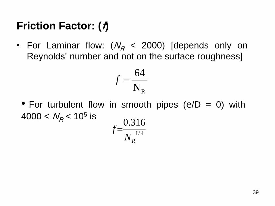
Friction Factor: (f)

• For Laminar flow: (NR < 2000) [depends only on

Reynolds’ number and not on the surface roughness]

RN

64f

• For turbulent flow in smooth pipes (e/D = 0) with

4000 < NR < 105 is

4/1

316.0

RNf

40

2.51log2

1 fN

f

R

510e

7.3log21

RNfor

D

f

• Colebrook-White Equation for f

fND

e

f R

51.2

7.3ln86.0

1

For turbulent flow ( NR > 4000 ) with e/D > 0.0, the friction factor

can be founded from:

• Th.von Karman formulas:

There is some difficulty in solving this equation

So, Miller improve an initial value for f , (fo) 2

9.0

74.5

7.3log25.0

R

oND

ef

The value of fo can be use directly as f if: 26

83

101101

101104

-

R

D e

N

Friction Factor f

e7.1'

ee 7.108.0 '

RN

f64

pipe wall

e

51.2log2

110

fN

f

R

e

pipe wall

transitionally

rough

e

pipe wall

rough

f independent of relative

roughness e/D

f independent of NR

f varies with NR and e/D

turbulent flow

NR > 4000

laminar flow

NR < 2000

e08.0'

e

D

f7.3log2

110

fN

D

e

fR

51.2

7.3log2

110

Colebrook formula

The thickness of the laminar sublayer decrease with an increase in NR

Smooth

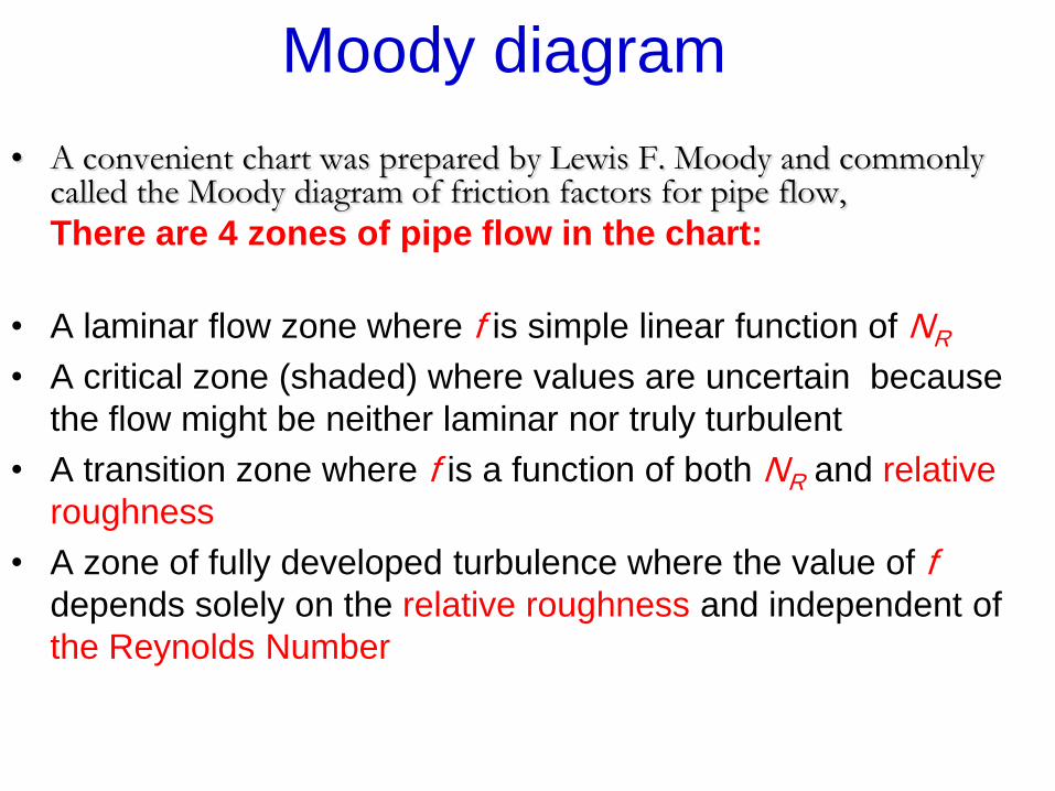
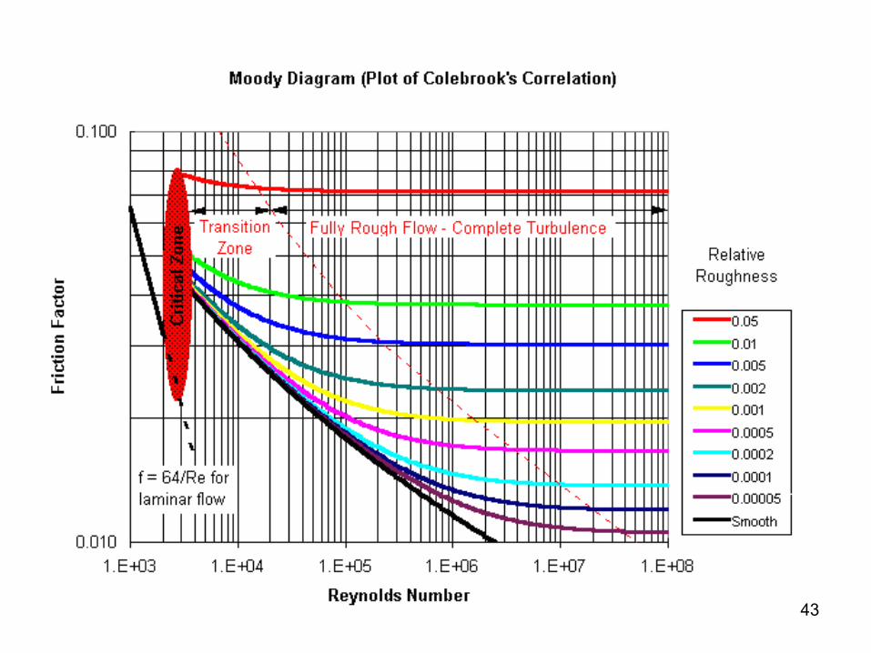
Moody diagram

• A convenient chart was prepared by Lewis F. Moody and commonly called the Moody diagram of friction factors for pipe flow,

There are 4 zones of pipe flow in the chart:

• A laminar flow zone where f is simple linear function of NR

• A critical zone (shaded) where values are uncertain because

the flow might be neither laminar nor truly turbulent

• A transition zone where f is a function of both NR and relative

roughness

• A zone of fully developed turbulence where the value of f depends solely on the relative roughness and independent of

the Reynolds Number

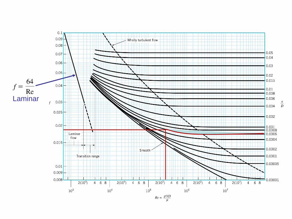
Laminar

45

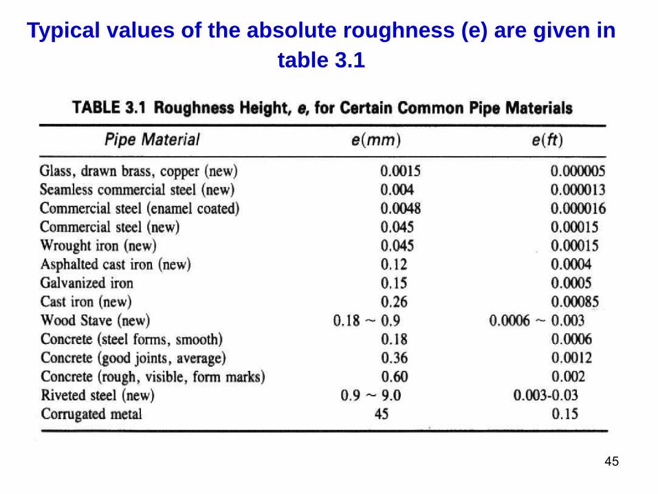
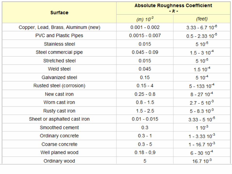
Typical values of the absolute roughness (e) are given in

table 3.1

47

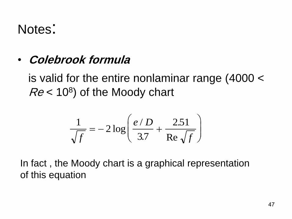
Notes:

• Colebrook formula

is valid for the entire nonlaminar range (4000 <

Re < 108) of the Moody chart

12

37

2 51

f

e D

f

log

/

.

.

Re

In fact , the Moody chart is a graphical representation

of this equation

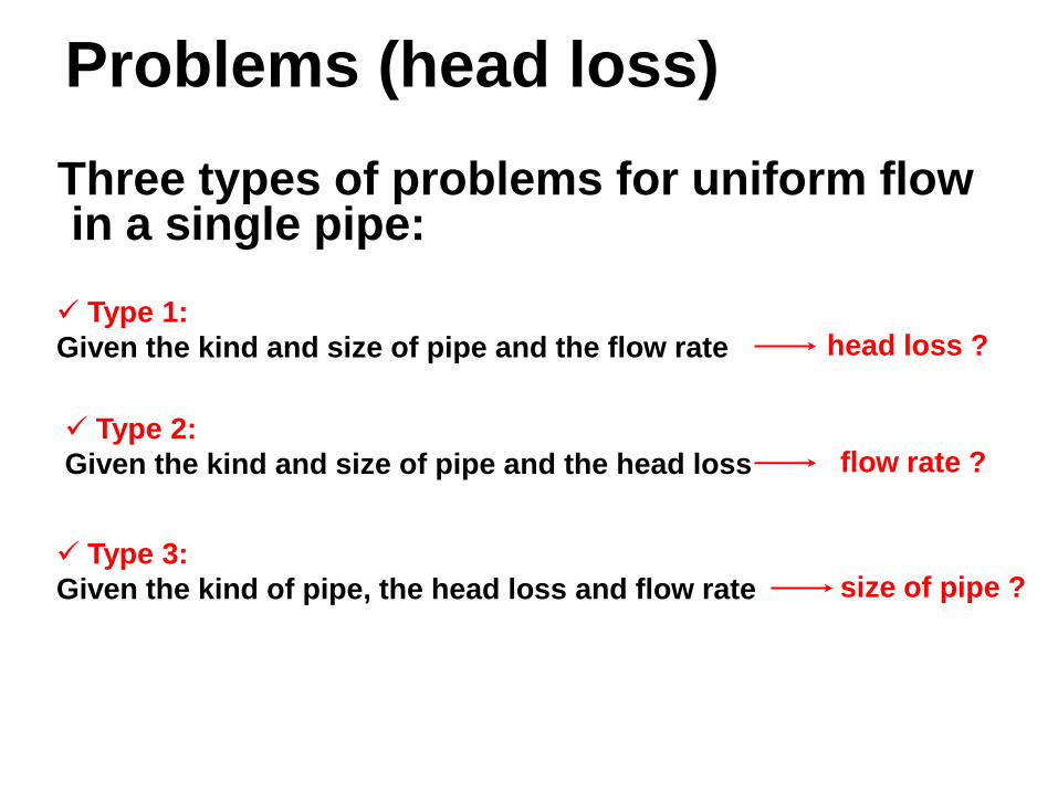
Problems (head loss)

Three types of problems for uniform flow in a single pipe:

Type 1:

Given the kind and size of pipe and the flow rate head loss ?

Type 2:

Given the kind and size of pipe and the head loss flow rate ?

Type 3:

Given the kind of pipe, the head loss and flow rate size of pipe ?

50

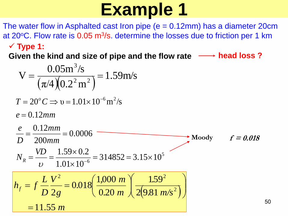
The water flow in Asphalted cast Iron pipe (e = 0.12mm) has a diameter 20cm

at 20oC. Flow rate is 0.05 m3/s. determine the losses due to friction per 1 km

Example 1

1.59m/s

m0.2π/4

/s0.05mV

22

3

5

6

26

1015.33148521001.1

2.059.1

0006.0200

12.0

12.0

/sm101.01υ20

VDN

mm

mm

D

e

mme

CT

R

o

f = 0.018 Moody

m

m/s.

.

m.

m,.

g

V

D

Lfh f

55.11

8192

591

200

00010180

2 2

22

Type 1:


The water flow in commercial steel pipe (e = 0.045mm) has a diameter 0.5m at 20oC. Q=0.4 m3/s. determine the losses due to friction per 1 km

sm

A

QV / 037.2

45.0

4.0

2

013.0

109105.0

045.0

10012.110006.1

037.25.0

10006.15.4220

10497

5.42

10497

5

3

6

6

6

5.1

6

5.1

6

f

D

e

N

T

Moody

R

kmmh f / 5.581.92

037.2

5.0

1000013.0

2

Example 2

Type 1:


fRD

k

f e

s 51.2

7.3ln86.0

1

Use other methods to solve f

01334.0

10012.1

74.5

7.3

109log25.0

74.5

7.3log25.0

2

9.06

52

9.0

e

s

oR

Dkf

678.866.8

01334.0

51.2

7.3

109ln86.0

01334.0

1 5

eR

1- Cole brook

kmmh f / 5.581.92

037.2

5.0

100001334.0

2

fND

e

f R

51.2

7.3ln86.0

1

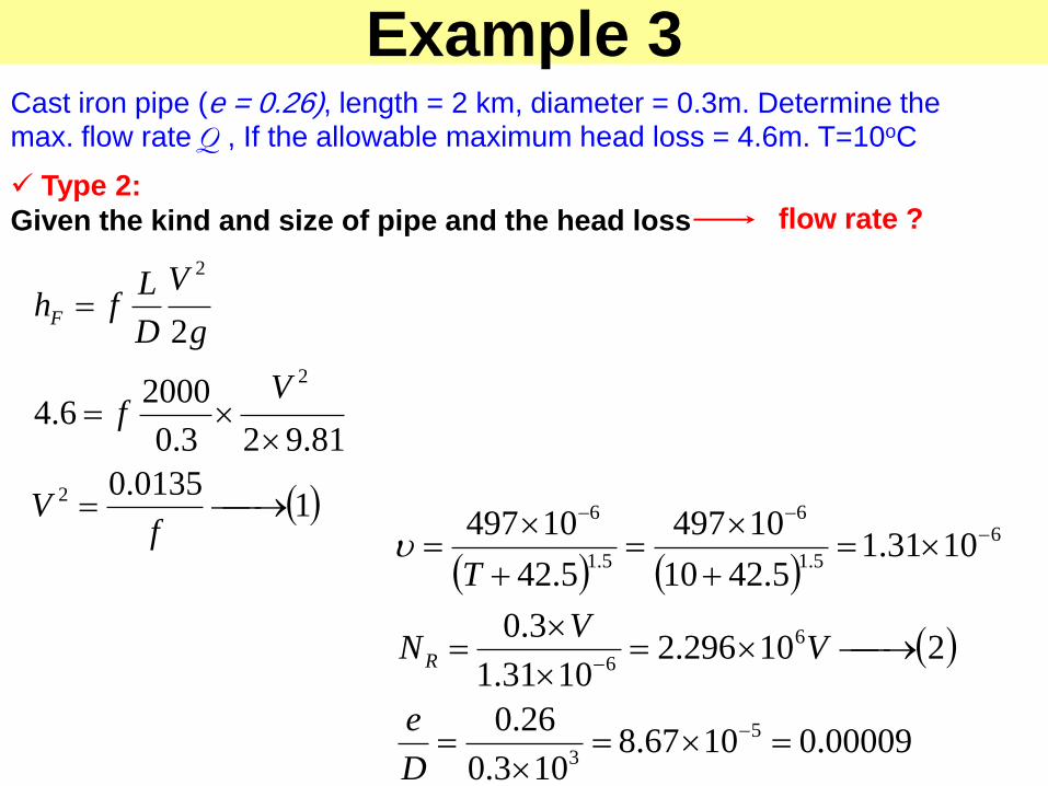
Cast iron pipe (e = 0.26), length = 2 km, diameter = 0.3m. Determine the max. flow rate Q , If the allowable maximum head loss = 4.6m. T=10oC

10135.0

81.923.0

20006.4

2

2

2

2

fV

Vf

g

V

D

LfhF

00009.01067.8103.0

26.0

210296.21031.1

3.0

1031.15.4210

10497

5.42

10497

5

3

6

6

6

5.1

6

5.1

6

D

e

VV

N

T

R

Example 3

Type 2:


02.0

1067.8

10668.2

m/s 16.101.0

4

52

1

f

D

e

N

Vf

Moody

R

eq

eq

021.0

1067.8

10886.1

m/s 82.002.0

4

52

1

f

D

e

N

Vf

Moody

R

eq

eq

10135.02 f

V

210296.2 6 VNR

Trial 1

Trial 2

V= 0.82 m/s , Q = V*A = 0.058 m3/s

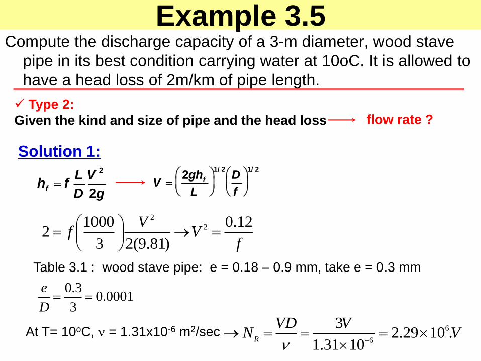
Example 3.5 Compute the discharge capacity of a 3-m diameter, wood stave

pipe in its best condition carrying water at 10oC. It is allowed to

have a head loss of 2m/km of pipe length.

hf fL

D

V 2

2g

V 2ghf

L

1/ 2D

f

1/ 2

fV

Vf

12.0

)81.9(23

10002 2

2

Table 3.1 : wood stave pipe: e = 0.18 – 0.9 mm, take e = 0.3 mm

Solution 1:

0001.03

3.0

D

e

At T= 10oC, = 1.31x10-6 m2/sec VVVD

NR

.1029.21031.1

3 6

6

Type 2:


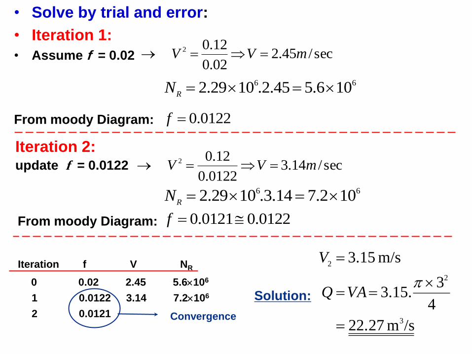
• Solve by trial and error:

• Iteration 1:

• Assume f = 0.02 sec/45.202.0

12.02 mVV

66 106.545.2.1029.2 R

N

From moody Diagram: 0122.0f

Iteration 2: update f = 0.0122 sec/14.3

0122.0

12.02 mVV

66 102.714.3.1029.2 R

N

From moody Diagram: 0122.00121.0 f

0 0.02 2.45 5.6106

1 0.0122 3.14 7.2106

2 0.0121

Iteration f V NR

Convergence

Solution:

/sm 2.272

4

3.15.3

m/s 15.3

3

2

2

VAQ

V

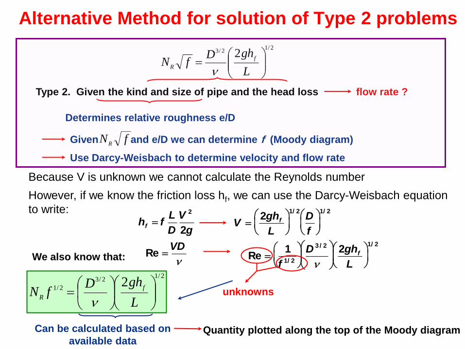
flow rate ?

Determines relative roughness e/D

2/12/3 2

L

ghDfN

f

R

Type 2. Given the kind and size of pipe and the head loss

Given and e/D we can determine f (Moody diagram) fNR

Use Darcy-Weisbach to determine velocity and flow rate

Alternative Method for solution of Type 2 problems

Because V is unknown we cannot calculate the Reynolds number

However, if we know the friction loss hf, we can use the Darcy-Weisbach equation

to write:

hf fL

D

V 2

2g

V 2ghf

L

1/ 2D

f

1/ 2

We also know that:

Re VD

Re 1

f 1/ 2

D 3 / 2

2ghf

L

1/ 2

unknowns

2/12/3

2/12

L

ghDfN

f

R

Can be calculated based on

available data Quantity plotted along the top of the Moody diagram

Moody Diagram

Smooth pipes

Fully rough pipes

Resis

tan

ce C

oeff

icie

nt

f

Reynolds number

Rela

tive r

ou

gh

ness e

/D

2/12/3

2/12

L

ghDfN

f

R

Example 3.5 Compute the discharge capacity of a 3-m diameter, wood stave pipe in its best

condition carrying water at 10oC. It is allowed to have a head loss of 3m/km

of pipe length.

5

6

232/1

2/3

1062.91000

)3)(81.9(2

1031.1

)3(2

L

ghDfN

f

R

Table 3.1 : wood pipe: e = 0.18 – 0.9 mm, take e = 0.3 mm

Solution 2:

0001.03

3.0

D

e

Type 2: Given the kind and size of pipe and the head loss flow rate ?

At T= 10oC, = 1.31x10-6 m2/sec

From moody Diagram: 0121.0f

sec/15.32

2

2/12/12

mf

D

L

ghV

g

V

D

Lfh

f

f

/sm 2.272

4

3.15.3,

3

2

VAQ

f = 0.0121

Example (type 2)

H

L

H = 4 m, L = 200 m, and D = 0.05 m

What is the discharge through the

galvanized iron pipe?

Table : Galvanized iron pipe: e = 0.15 mm e/D = 0.00015/0.05 = 0.003

= 10-6 m2/s

We can write the energy equation between the water surface in the reservoir and the

free jet at the end of the pipe:

Lh

g

Vh

p

g

Vh

p

22

2

2

2

2

2

1

1

1

g

V

D

Lf

g

V

2200040

22

2

f

D

Lf

gV

40001

5.78

1

422

1

2

Example (continued) Assume Initial value for f : fo = 0.026

Initial estimate for V: m/sec 865.0026.040001

5.78

V

Calculate the Reynolds number 44 103.4105 V

DVN

R

Updated the value of f from the Moody diagram f1 = 0.029

m/sec 819.0029.040001

5.78

V

442 101.4105 VDV

NR

0 0.026 0.865 4.3104

1 0.029 0.819 4.1104

2 0.0294 0.814 4.07104

3 0.0294

Iteration f V NR

Convergence

Solution:

V2 0.814 m/s

Q VA 0.814 0.052

4

1.60103 m3 /s

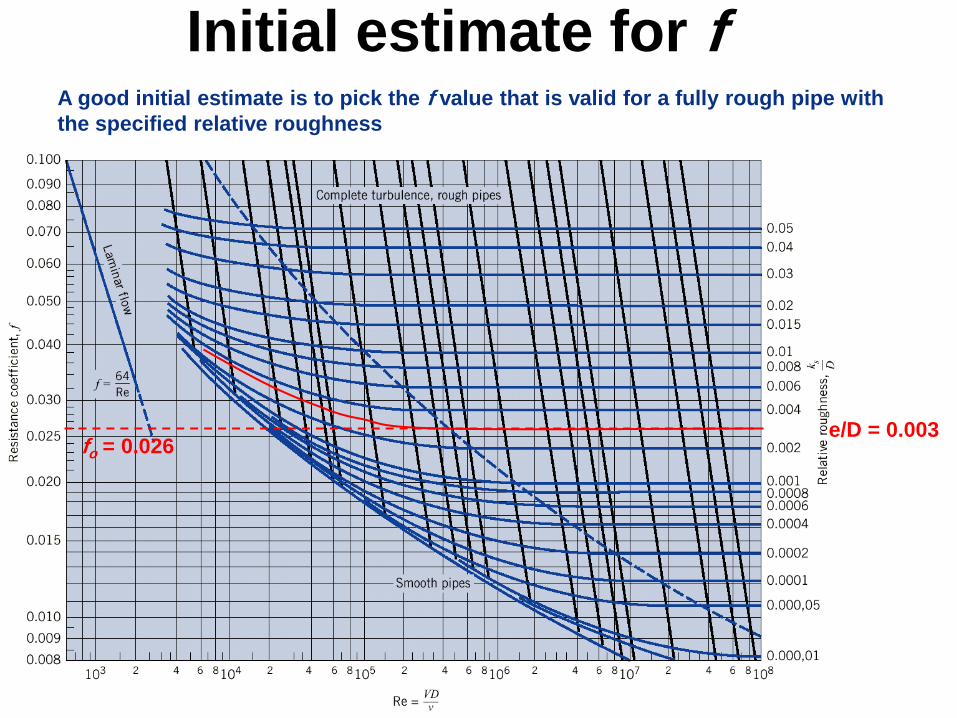
e/D = 0.003

Initial estimate for f A good initial estimate is to pick the f value that is valid for a fully rough pipe with

the specified relative roughness

fo = 0.026

Solution of Type 3 problems-uniform flow in a

single pipe

Given the kind of pipe, the head loss and flow rate size of pipe ?

Determines

equivalent roughness e

Problem? Without D we cannot calculate the relative

roughness e/D, NR, or fNR

Solution procedure: Iterate on f and D

1. Use the Darcy Weisbach equation and guess an initial value for f 2. Solve for D

3. Calculate e/D

4. Calculate NR

5. Update f 6. Solve for D

7. If new D different from old D go to step 3, otherwise done

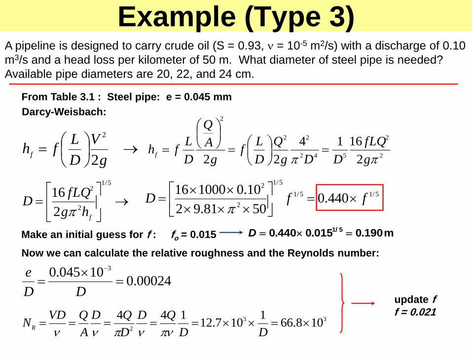
Example (Type 3) A pipeline is designed to carry crude oil (S = 0.93, = 10-5 m2/s) with a discharge of 0.10

m3/s and a head loss per kilometer of 50 m. What diameter of steel pipe is needed?

Available pipe diameters are 20, 22, and 24 cm.

From Table 3.1 : Steel pipe: e = 0.045 mm

Darcy-Weisbach:

g

V

D

Lfh

f2

2

2

2

542

22

2

2

1614

22 g

fLQ

DDg

Q

D

Lf

g

A

Q

D

Lfh

f

5/1

2

2

2

16

fhg

fLQD

5/15/1

5/1

2

2

440.05081.92

10.0100016ffD

Make an initial guess for f : fo = 0.015

D 0.440 0.0151/ 5 0.190 m

Now we can calculate the relative roughness and the Reynolds number:

33

2108.66

1107.12

144

DD

QD

D

QD

A

QVDN

R

00024.010045.0 3

DD

e

update f f = 0.021

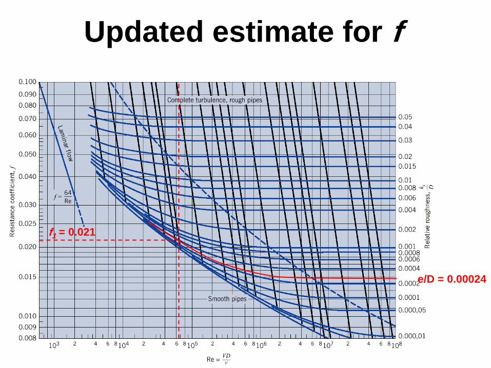
e/D = 0.00024

Updated estimate for f

f1 = 0.021

0 0.015 0.190 66.8103 0.00024

Iteration f D NR e/D

Example Cont’d

5/1440.0 fD

update f

DN

R

1107.12 3

From moody diagram, updated estimated for f :

f1 = 0.021 D = 0.203 m

3105.62 R

N

00023.0D

e

1 0.021 0.203 62.5103 0.00023

2 0.021 Convergence

Solution:

D = 0.203m

Use next larger commercial

size:

D = 22 cm

Example 3.6 Estimate the size of a uniform, horizontal welded-steel pipe installed to carry 14

ft3/sec of water of 70oF (20oC). The allowable pressure loss is 17 ft/mi of

pipe length.

From Table : Steel pipe: e = 0.046 mm

Darcy-Weisbach:

hL fL

D

V 2

2g

Q VA

hL fL

D

Q

A

2

2g f

L

D

Q 2

2g

42

2D 4

1

D 5

16fLQ 2

2g 2

5/1

2

28

Lhg

fLQD

afff

D 5/15/1

5/1

2

2

33.41781.9

1452808

Let D = 2.5 ft, then V = Q/A = 2.85 ft/sec

Now by knowing the relative roughness and the Reynolds number:

5

510*6.6

10*08.1

5.2*85.2

VDNR

0012.05.2

003.0

D

e

We get f =0.021

Solution 2:

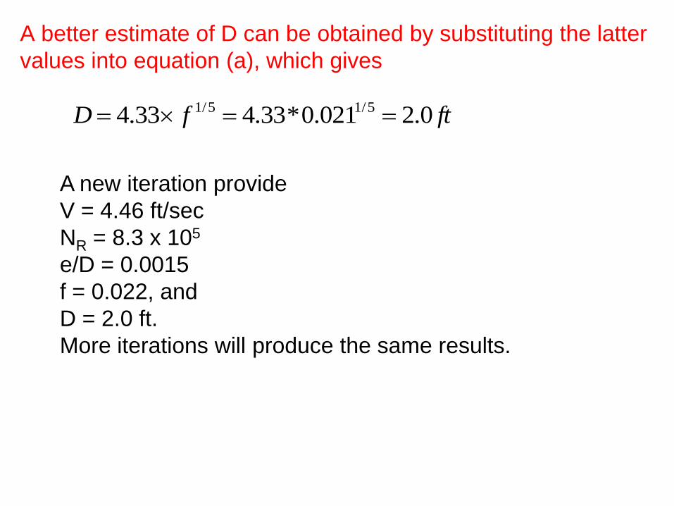
A better estimate of D can be obtained by substituting the latter

values into equation (a), which gives

ftfD 0.2021.0*33.433.4 5/15/1

A new iteration provide

V = 4.46 ft/sec

NR = 8.3 x 105

e/D = 0.0015

f = 0.022, and

D = 2.0 ft.

More iterations will produce the same results.

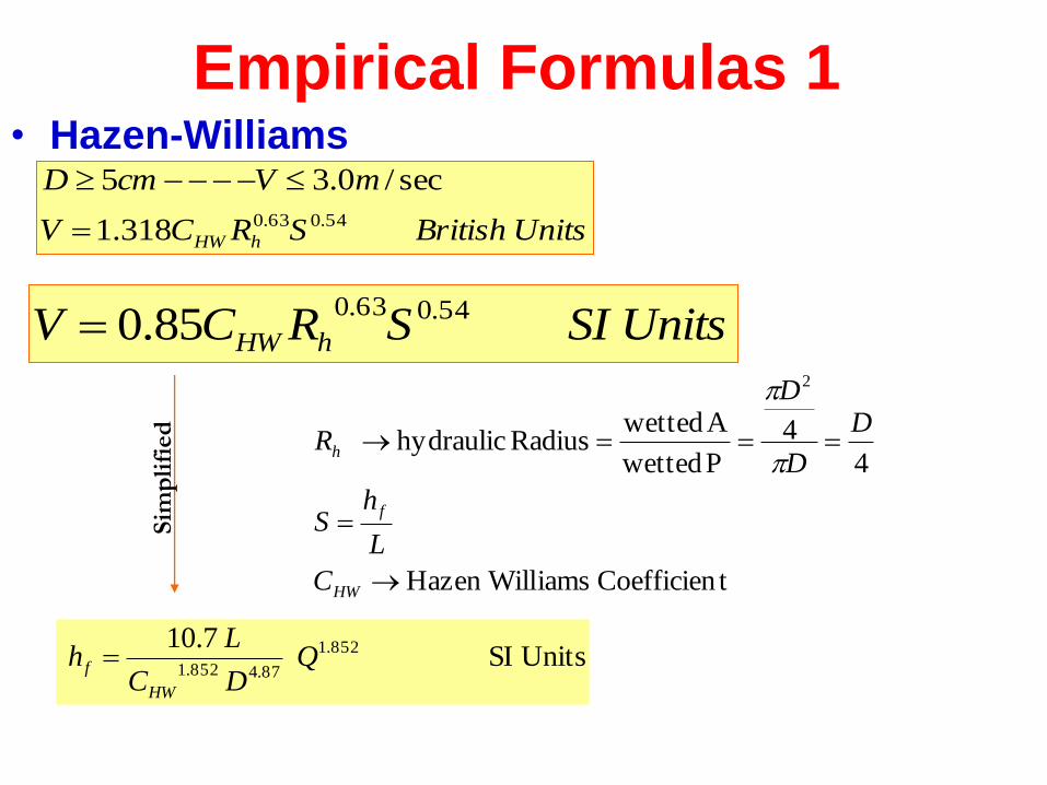
Empirical Formulas 1 • Hazen-Williams

UnitsSISRCV hHW

54.063.085.0

tCoefficien iamsHazen Will

4

4

P wetted

A wetted Radius hydraulic

2

C

L

hS

D

D

D

R

HW

f

h

UnitsSI

0.71 852.1

87.4852.1Q

DC

Lh

HW

f

Sim

pli

fied

UnitsBritishSRCV

mVcmD

hHW

54.063.0318.1

sec/0.35

Empirical Formulas 2

72

Manning Formula

• This formula has extensively been used

for open channel designs

• It is also quite commonly used for pipe

flows

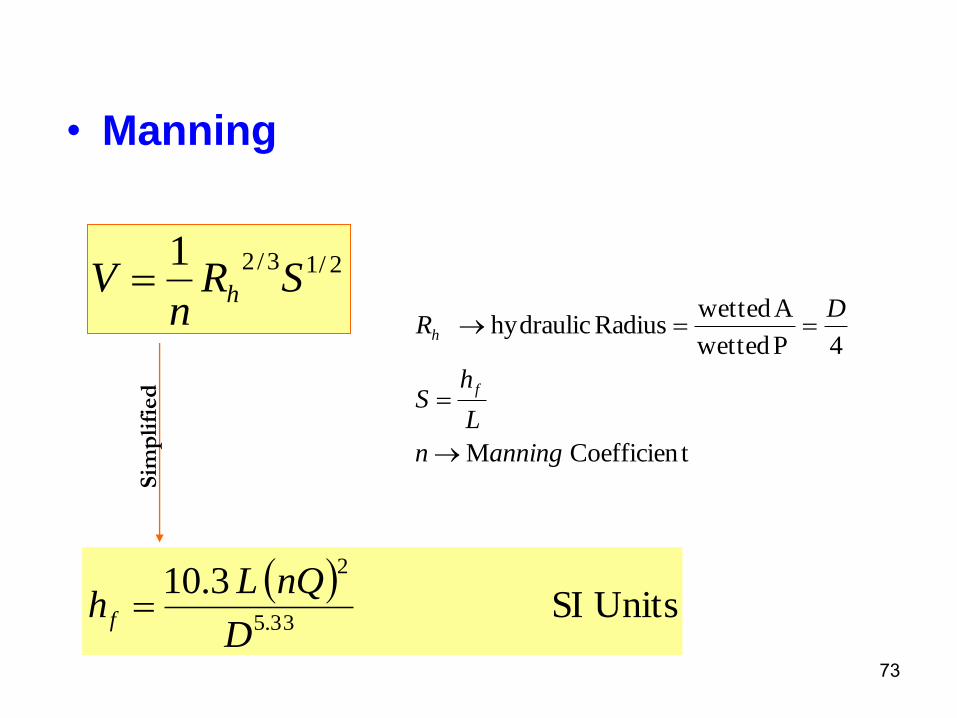
73

• Manning

tCoefficien M

4 P wetted

A wetted Radius hydraulic

anningn

L

hS

D

R

f

h

Sim

pli

fied

UnitsSI

0.3133.5

2

D

nQLh f

2/13/21SR

nV h

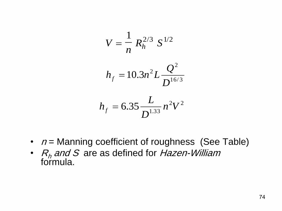
74

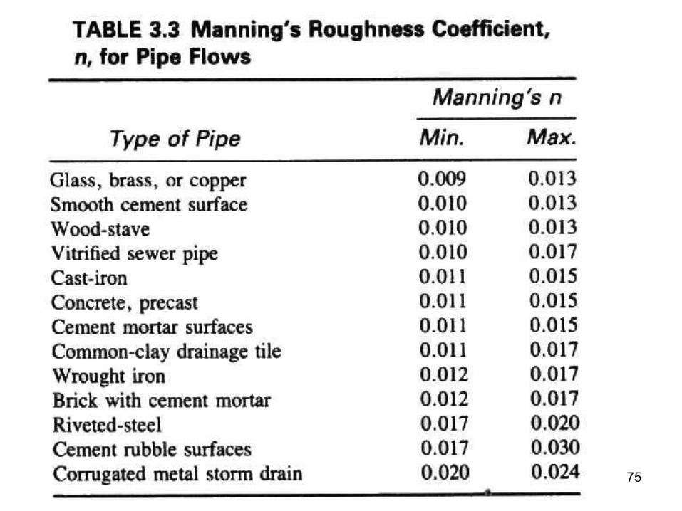
• n = Manning coefficient of roughness (See Table) • Rh and S are as defined for Hazen-William

formula.

Vn

R Sh1 2 3 1 2/ /

3/16

223.10

D

QLnh f

22

33.135.6 Vn

D

Lh f

76

The Chezy Formula

V C R Sh 1 2 1 2/ /

2

4

C

V

D

Lh f

where C = Chezy coefficient

77

• It can be shown that this formula, for circular pipes, is

equivalent to Darcy’s formula with the value for

[f is Darcy Weisbeich coefficient]

• The following formula has been proposed for the value of

C:

[n is the Manning coefficient]

Cg

f

8

C S n

S

n

Rh

23000155 1

1 23000155

.

(.

)

78

The Strickler Formula:

V k R Sstr h 2 3 1 2/ /

2

33.135.6

str

fk

V

D

Lh

where kstr is known as the Strickler coefficient.

Comparing Manning formula and Strickler formula, we can see that

1

nkstr

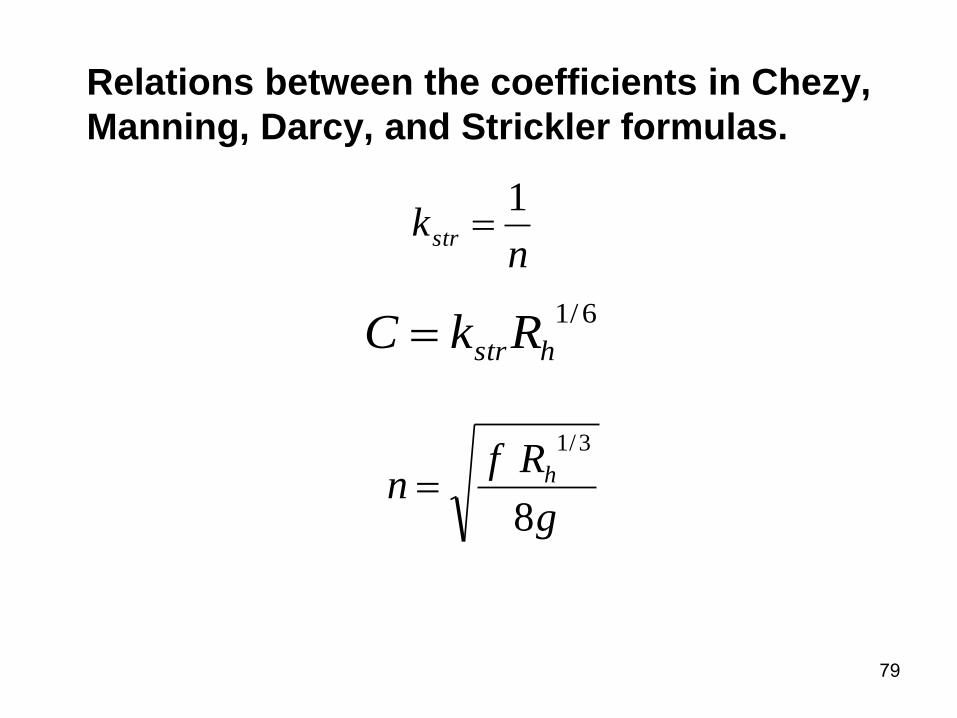
79

Relations between the coefficients in Chezy,

Manning, Darcy, and Strickler formulas.

nkstr

1

6/1

hstrRkC

g

Rfn h

8

3/1

Example

New Cast Iron (CHW = 130, n = 0.011) has length = 6 km and diameter = 30cm.

Q= 0.32 m3/s, T=30o. Calculate the head loss due to friction using:

a) Hazen-William Method

b) Manning Method

33332030130

6000710

710

8521

8748521

8521

8748521

m . .

. h

Q DC

L.h

.

..f

.

..

HW

f

m

.

.. .h

D

nQ L h

.f

.f

47030

32001106000310

3.10

335

2

335

2

82

Minor losses

It is due to the change

of the velocity of the

flowing fluid in the

magnitude or in

direction [turbulence

within bulk flow as it

moves through and

fitting] Flow pattern through a valve

83

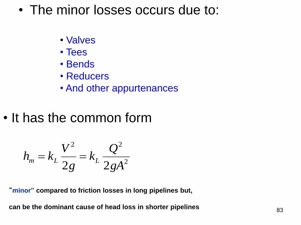
• The minor losses occurs due to:

• Valves

• Tees

• Bends

• Reducers

• And other appurtenances

• It has the common form

2

22

22 gA

Qk

g

Vkh LLm

can be the dominant cause of head loss in shorter pipelines

“minor” compared to friction losses in long pipelines but,

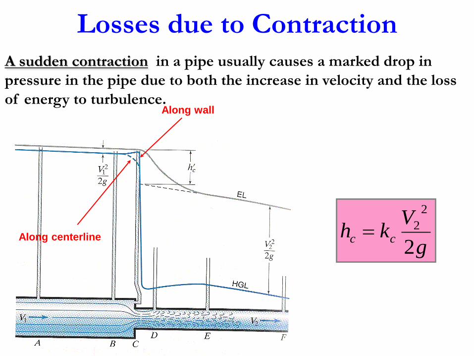
Losses due to Contraction A sudden contraction in a pipe usually causes a marked drop in

pressure in the pipe due to both the increase in velocity and the loss

of energy to turbulence.

g

Vkh cc

2

2

2Along centerline

Along wall

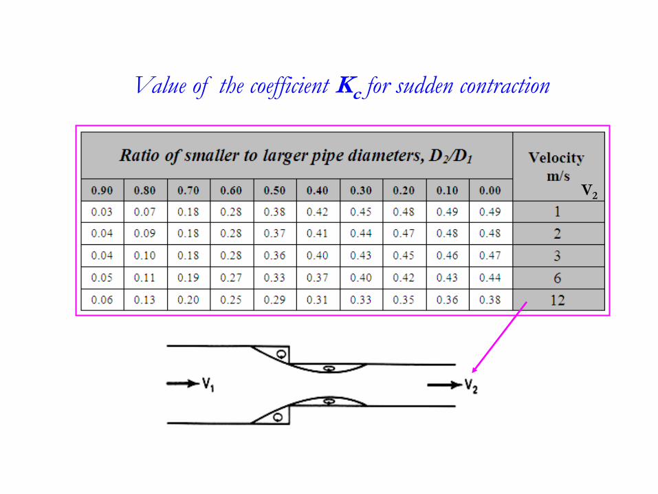
Value of the coefficient Kc for sudden contraction

V2

86

Max Head Loss Due to a Sudden Contraction

h KV

gL L

22

2

g

Vhc

2 5.0

22

Head losses due to pipe contraction may be greatly reduced

by introducing a gradual pipe transition known as a confusor

g

V'k'h cc

2

2

2

'kc

Figure 3.11

Losses due to Enlargement

g

VVhE

2

)( 2

21

A sudden Enlargement in a pipe

Note that the drop in the energy line is much

larger than in the case of a contraction

abrupt expansion

gradual expansion

smaller head loss than in the case of an abrupt expansion

Head losses due to pipe enlargement may be greatly reduced by

introducing a gradual pipe transition known as a diffusor

g

VV'k'h EE

2

2

2

2

1

91

Loss due to pipe entrance

General formula for head loss at the entrance of a pipe is also

expressed in term of velocity head of the pipe

g

VKh entent

2

2

92

Head Loss at the Entrance of a Pipe (flow leaving a tank)

Reentrant

(embeded)

KL = 0.8

Sharp

edge

KL = 0.5

Well

rounded

KL = 0.04

Slightly

rounded

KL = 0.2

h KV

gL L

2

2

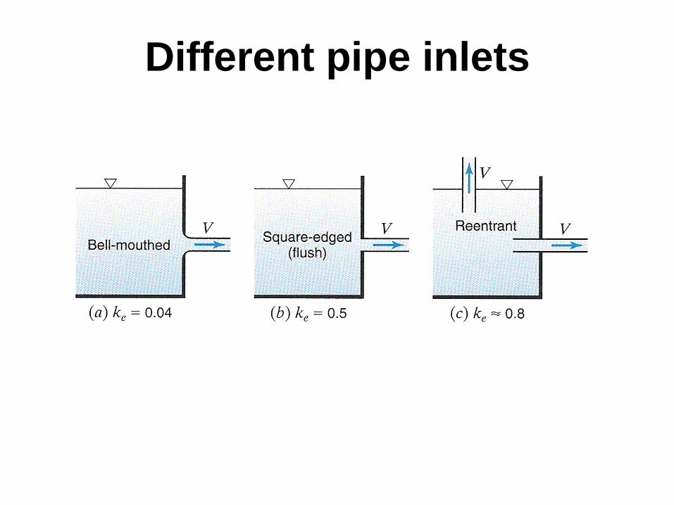
Different pipe inlets

increasing loss coefficient

94

Another Typical values for various amount of rounding of

the lip

95

Head Loss at the Exit of a Pipe

(flow entering a tank)

hV

gL

2

2

the entire kinetic energy of the exiting fluid (velocity V1) is

dissipated through viscous effects as the stream of fluid mixes

with the fluid in the tank and eventually comes to rest (V2 = 0).

KL = 1.0 KL = 1.0

KL = 1.0 KL = 1.0

96

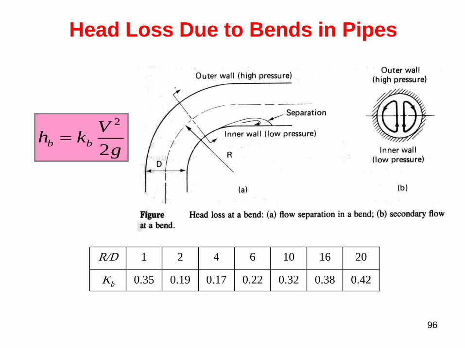
Head Loss Due to Bends in Pipes

R/D 1 2 4 6 10 16 20

Kb 0.35 0.19 0.17 0.22 0.32 0.38 0.42

g

Vkh bb

2

2

97

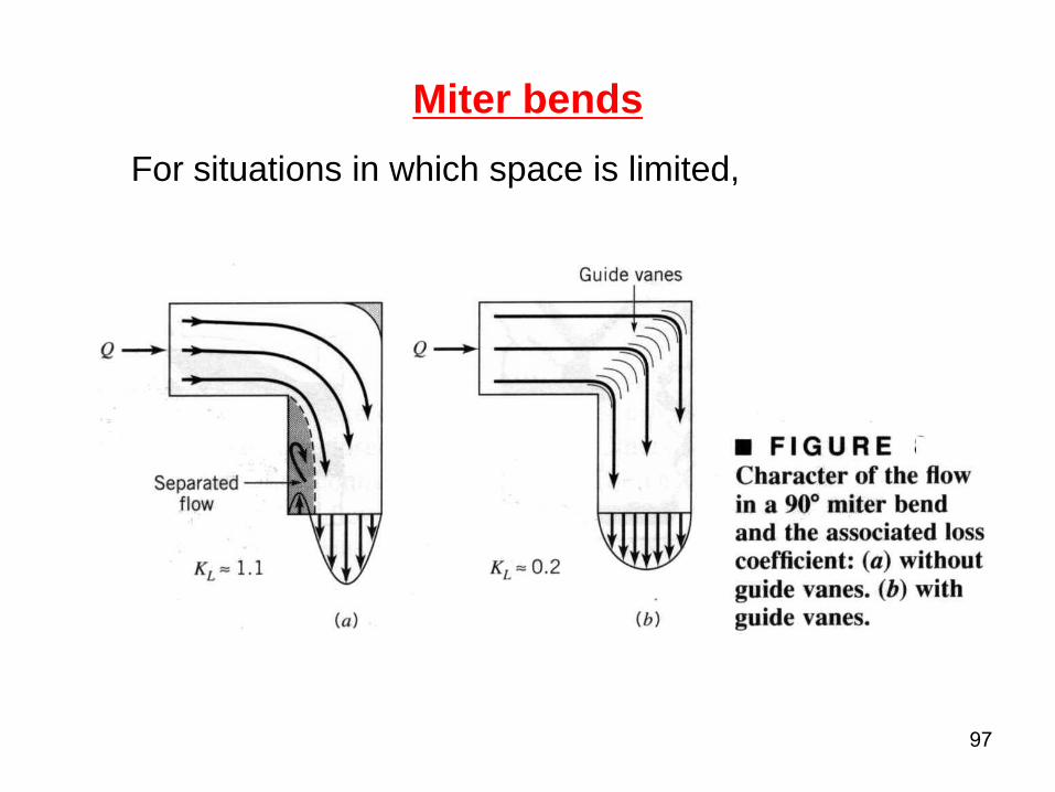
Miter bends

For situations in which space is limited,

98

Head Loss Due to Pipe Fittings

(valves, elbows, bends, and tees)

h KV

gv v

2

2

100

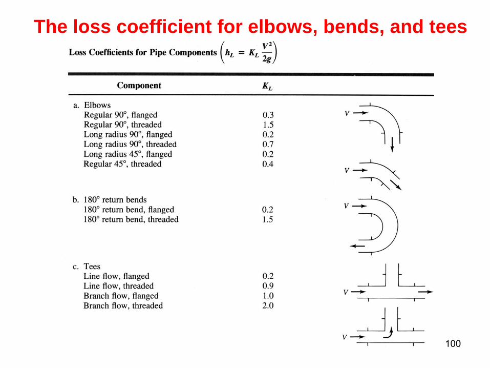
The loss coefficient for elbows, bends, and tees

Loss coefficients for pipe components (Table)

Minor loss coefficients (Table)

Minor loss calculation using equivalent

pipe length

f

DkL l

e

Energy and hydraulic grade lines

Unless local effects are of particular interests, the

changes in the EGL and HGL are often shown as

abrupt changes (even though the loss occurs over

some distance)

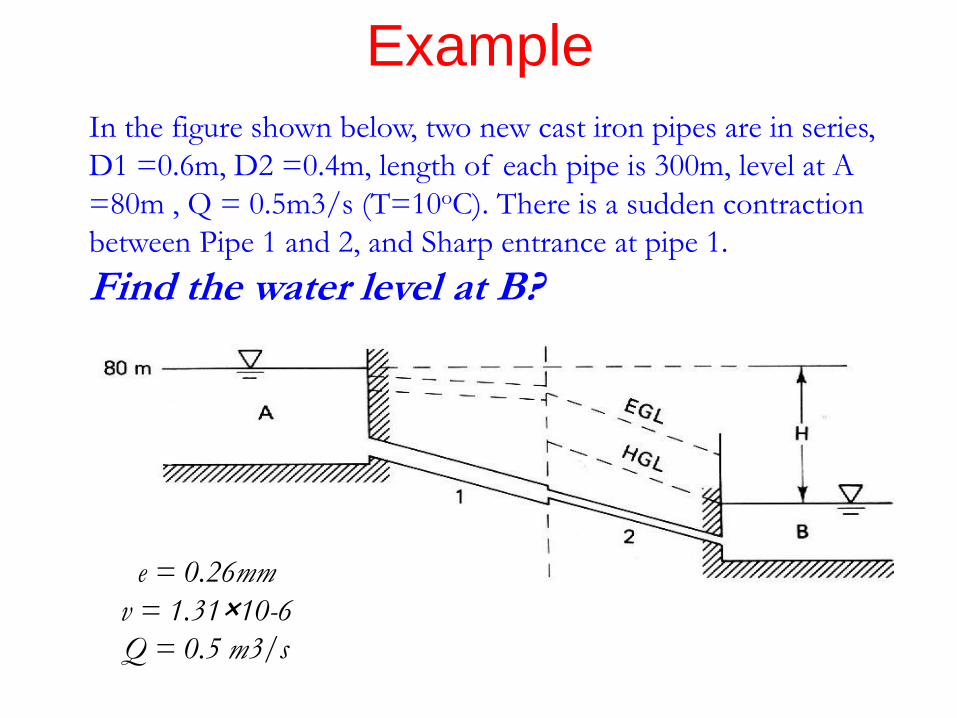
Example

In the figure shown below, two new cast iron pipes are in series,

D1 =0.6m, D2 =0.4m, length of each pipe is 300m, level at A

=80m , Q = 0.5m3/s (T=10oC). There is a sudden contraction

between Pipe 1 and 2, and Sharp entrance at pipe 1.

Find the water level at B?

e = 0.26mm

v = 1.31×10-6 Q = 0.5 m3/s

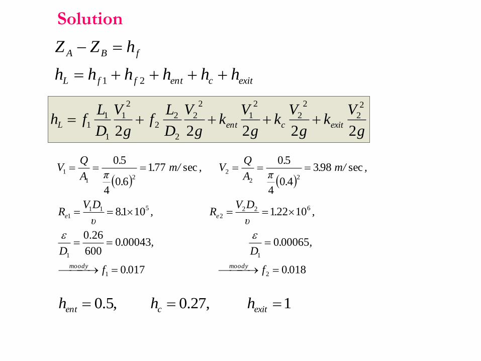
exitcentffL

fBA

hhhhhh

hZZ

21

g

Vk

g

Vk

g

Vk

g

V

D

Lf

g

V

D

Lfh exitcentL

22222

2

2

2

2

2

1

2

2

2

22

2

1

1

11

01800170

000650000430600

26.0

102211018

sec983

404

50sec771

604

50

21

11

6222

5111

22

22

1

1

.f .f

,.D

, .D

,.υ

DV R , .

υ

DVR

, m/.

.π

.

A

Q, V m/.

.π

.

A

QV

moodymoody

ee

1 ,27.0 ,5.0 exitcent hhh

Solution

m.g

.

g

..

g

..

g

. .

. .

g

. .

. .h f

36132

983

2

983270

2

77150

2

983

40

3000180

2

771

60

3000170

222

22

ZB = 80 – 13.36 = 66.64 m

g

Vk

g

Vk

g

Vk

g

V

D

Lf

g

V

D

Lfh exitcentL

22222

2

2

2

2

2

1

2

2

2

22

2

1

1

11

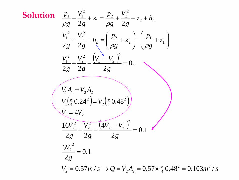
Example

A pipe enlarge suddenly from D1=240mm to D2=480mm. the

H.G.L rises by 10 cm calculate the flow in the pipe

smAVQsmV

g

V

g

VV

g

V

g

V

VV

VV

AVAV

g

VV

g

V

g

V

zg

pz

g

ph

g

V

g

V

hzg

V

g

pz

g

V

g

p

L

L

/103.048.057.0/57.0

1.02

6

1.02

4

22

16

4

48.024.0

1.0222

22

22

32

4222

2

2

2

22

2

2

2

2

21

2

42

2

41

2211

2

21

2

2

2

1

11

22

2

2

2

1

2

2

221

2

11

Solution

110

• Note that the above values are average

typical values, actual values will depend

on the manufacturer of the components.

• See:

– Catalogs

– Hydraulic handbooks !!

chapter 3 water flow in pipes - islamic university of...

Documents