75

CHAPTER 3

RESERVOIR

3.1 Introduction

A reservoir is a large, artificial lake created by constructing a dam across a river (Fig. 3.1). Broadly speaking, any water pool or a lake may be termed a reservoir. However, the term reservoir in water resources engineering is used in a restricted sense for a comparatively large body of water stored on the upstream of a dam constructed for this purpose. Thus a dam and a reservoir exist together. The discharge in a river generally varies considerably during different periods of a year.

Fig. 3.1

If a reservoir serves only one purpose, it is called a single-purpose reservoir. On the other hand, if it serves more than one purpose, it is termed a multipurpose reservoir. The various purposes served by a multipurpose seservoir include (i) irrigation (ii) municipal and industrial water supply, (iii) flood control (iv) hydropower, (v) navigation, (vi) recreation, (vii) development of fish and wild life, (viii) soil conservation (ix) pollution control and (x) mosquito control.

3.2 Types of Reservoirs Depending upon the purpose served, the reservoirs may be broadly classified into five foutypes:

1. Storage (or conservation) reservoirs 2. Flood control reservoirs 3. Multipurpose reservoirs 4. Distribution reservoirs. 5. Balancing reservoirs

76

1. Storage reservoirs Storage reservoirs are also called conservation reservoirs because they are used to conserve water. Storage reservoirs are constructed to. Store the water in the rainy season and to release it later when the river flow is low store reservoirs are usually constructed for irrigation, the municipal water supply and hydropower. Although the storage reservoirs are constructed for storing water for various purposes, incidentally they also help in moderating the floods and reducing the flood damage to some extent on the downstream. However, they are not designed as flood control reservoirs.

2. Flood control reservoirs A flood control reservoir is constructed for the purpose of flood control It protects the areas lying on its downstream side from the damages due to flood. However, absolute protection from extreme floods is not economically feasible. A flood control reservoir reduces the flood damage, and it is also known as the flood-mitigation reservoir. Sometimes, it is called flood protection reservoir. In a flood control reservoir, the floodwater is discharged downstream till the outflow reaches the safe capacity of the channel downstream. When the discharge exceeds the safe capacity. The excess water is stored in the reservoir. The stored water is subsequently released when the inflow to reservoir decreases. Care is, however, taken that the discharge in the channel downstream, including local inflow, does not exceed its safe capacity. A flood control reservoir is designed to moderate the flood and not to conserve water. However, incidentally some storage is also done during the period of floods. Flood control reservoirs have relatively large sluice-way capacity to permit rapid drawdown before or after the occurrence of a flood.

3. Multipurpose Reservoirs A multipurpose reservoir is designed and constructed to serve two or more purposes. Most of the reservoirs are designed as multipurpose reservoirs to store water for irrigation and hydropower, and also to effect flood control.

4. Distribution Reservoir A distribution reservoir is a small storage reservoir to tide over the peak demand of water for municipal water supply or irrigation. The distribution reservoir is helpful in permitting the pumps to work at a uniform rate. It stores water during the period of lean demand and supplies the same during the period of high demand. As the storage is limited, it merely helps in distribution of water as per demand for a day or so and not for storing it for a long period. Water is pumped from a water source at a uniform rate throughout the day for 24 hours but the demand varies from time to time. During the period when the demand of water is less than the pumping rate, the water is stored in the distribution reservoir. On the other hand, when the demand of water is more than the pumping rate, the distribution reservoir is used for supplying water at rates greater than the pumping rate.

Distribution reservoirs are rarely used for the supply of water for irrigation. These are mainly used for municipal water supply.

5. Balancing reservoir A balancing reservoir is a small reservoir constructed d/s of the main reservoir for holding water released from the main reservoir.

77

3.3 Available Storage Capacity of a Reservoir

Whatever may be the use of a reservoir, its most important function is to store water during floods and to release it later. The storage capacity of a reservoir is, therefore, its most important characteristics. The available storage capacity of a reservoir depends upon the topography of the site and the height of dam. To determine the available storage capacity of a reservoir upto a certain level of water, engineering surveys are usually conducted.

For accurate determination of the capacity, a topographic survey of the reservoir area is usually conducted, and a contour map of the area is prepared. A contour plan of the area is prepared to a scale of 1 cm = 100 m or 150 m with a contour interval of 1 to 3 m, depending upon the size of the reservoir. The storage capacity and the water spread area at different elevations can be determined from the contour map, as explained below.

(a) Area-Elevation Curve From the contour plan, the water spread area of the reservoir at any elevation is determined by measuring the area enclosed by the corresponding contour. Generally, a planimeter is used for measuring the area. An elevation-area curve is then drawn between the surface area as abscissa and the elevation as ordinate (Fig. 3.2)

Fig. 3.2

(b) Elevation-Capacity Curve The storage capacity of the reservoir at any elevation is determined from the water spread area at various elevations. The following formulae are commonly used to determine the storage capacity (i.e. storage volumes).

1. Trapezoidal formula According to the trapezoidal formula, the storage volume between two successive contours of areas A1, and A2 is given by

)( 211 2AA

hV +=∆ (3.1)

where h is the contour interval.

Therefore, the total volume V of the storage is given by

78

V = ∆V1 + ∆V2 + ∆V3 +............. = Σ∆V

or V = 2h

[ A1 + 2A2 + 2A3 +...............+2 An-1 + An ] (3.2)

where n is the total number of areas.

2. Cone formula According to the cone formula, the storage volume between two successive contours of areas A1 and A2 is given by

∆V1 = )( 21213AAAA

h++ (3.3)

The total volume V is given by

V = ∆V1 + ∆V2 + ∆V3 +............. = Σ∆V (3.4)

3. Prismoidal formula According to the prismoidal formula, the storage volume between 3 successive contours is given by

∆V1 = 321 4(3

AAAh

++ )

The total volume is given by

V = 3h

[( A1 + An)+4(A2 + A4 +. A6 +.......) + 2 (A3 + A5 + .....)] (3.6)

where A3, A5, etc are the areas with odd numbers : A2, A4, A6, etc are the areas with even numbers A1 and An are respectively, the first and the last area.

The prismoidal formula is applicable only when there are odd numbers of areas ( i.e. n should be an odd number). In the case of even number of areas, the volume upto the last but one area is determined by the prismoidal formula, and that of the last segment is determined by the trapezoidal formula.

Storage Volume from cross-sectional areas In the absence of adequate contour maps, the storage volume can be computed from the cross-sectional areas of the river. Cross-sectional areas are obtained from the cross-sections of the river taken upstream of the dam up to the u/s end of the reservoir. The volume is determined from the prismoidal formula,

V = 3d

[( A1 + An)+4(A2 + A4 +.......) + 2 (A3 + A5 + .....)] (3.7)

where A1, A2 etc. are the area of the cross-section of the river up o the full reservoir level and d

79

is the distance between the sections. The formula is applicable for odd number of sections.

An elevation-storage volume is plotted between the storage volume as abscissa and the elevations as ordinate (Fig. 3.3) Generally, the volume is calculated in Mm3 or M ha-m.

Fig. 3.3

(c) Combined Diagram It is the usual practice to plot both the elevation-area curve and the elevation-storage curve on the same paper (Fig. 3.4). The reader should carefully note the abscissa marking as the areas and volumes increase in the opposite directions:

Fig. 3.4

Submerged area In addition to finding out the capacity of a reservoir, the contour map of the reservoir can also be used to determine the land and property which would be submerged when the reservoir is filled upto various elevations. It would enable one to estimate the compensation to be paid to the owners of the submerged property and land. The time schedule according to which the areas should be evacuated, as the reservoir is gradually filled, can also be drawn.

Example 3.1 A reservoir has the following areas enclosed by contours at various elevations. Determine the capacity of the reservoir between elevations of 200.00 to 300.00.

80

Elevation 200.00 220.00 240.00 260.00 280.00 300.00 Area of contour

(km2) 150.00 175.00 210.00 270.00 320.00 400.00

Use (a) trapezoidal formula, (b) prismoidal formula

Solution (a) From Eq. 7.2, V = 2h

(A1 + 2A2 +2 A3 + 2A4 + 2A5 + A6)

= 220

(150 + 2 x 175 + 2 x 210 + 2 x 270 + 2 x 320 + 400)

= 25000 m-km2 = 25000 Mm3 = 2.5 Mha-m

(b) In this case, there are even number of areas. The prismoidal formula is applied to first 5 areas. From Eq. 3.6, considering the first 5 areas,

V1 = 3h

[(A1 + A5) + 4 (A2 + A4) + 2A3]

= 320

[(150.00 + 320.00) + 4(175 + 270) + 2 x 210]

= 17800 m-km2 = 17800 Mm3

Volume between the last two areas from Eq. 3.1,

V2 = 2h

(A5 + A6) = 220

(320 + 400) = 7200 m-km2

= 7200 Mm3

Total volume V = V1 + V2 = 17800 + 7200 =25000 Mm3 = 2.5 Mha-m

In this case, the computed volumes from both the methods are equal. In general, it is not always the case.

3.4 Investigations for Reservoir

The following investigations are usually conducted for reservoir planning. 1. Engineering surveys 2. Geological investigation 3. Hydrologic investigations

81

1. Engineering surveys Engineering surveys are conducted for the dam, the reservoir and other associated works. Generally, the topographic survey of the area is carried out and the contour plan is prepared. The horizontal control is usually provided by triangulation survey, and the vertical control by precise levelling.

(a) Dam site For the area in the vicinity of the dam site, a very accurate triangulation survey is conducted. A contour plan to a scale of 1/250 or 1/500 is usually prepared. The contour interval is usually 1 m or 2 m. The contour plan should cover an area at least upto 200 m upstream and 400m downstream and for adequate width beyond the two abutments.

(b) Reservoir For the reservoir, the scale of the contour plan is usually 1/15,000 with a contour interval of 2 m to 3 m, depending upon the size of the reservoir. The area-elevation and storage-elevation curves are prepared for different elevations upto an elevation 3 to 5m higher than the anticipated maximum water level (M.W.L).

2. Geological investigations Geological investigations of the dam and reservoir site are done for the following purposes. (i) Suitability of foundation for the dam. (ii) Watertightness of the reservoir basin (iii) Location of the quarry sites for the construction materials. 3. Hydrological investigations The hydrological investigations are conducted for the following purposes : (i) To study the runoff pattern and to estimate yield. (ii) To determine the maximum discharge at the site.

(i) Run off pattern and yield The most important aspect of the reservoir planning is to estimate the quantity of water likely to be available in the river from year to year and seasons to season. For the determination of the required storage capacity of a reservoir, the runoff pattern of the river at the dam site is required. If the stream gauging has been done for a number of years before the construction of the dam, the runoff pattern will be available from the record. It is generally assumed that the runoff pattern will be substantially the same in future also. The available record is used for estimating the storage capacity. The inflow hydrographs of two or three consecutive bad years when the discharge is low are frequently used for estimating the required capacity. However, if the stream gauging records are not available, the runoff and yield have to be estimated indirectly by the empirical (or) statistical methods. These are :

(i) Runoff expressed as a percentage of rainfall. (ii) Runoff expressed as a residual of rainfall after deducting losses due to evaporation,

transpiration and ground water accretion. (iii) Run off expressed as a function of mean annual temperature and rainfall.

(ii) Maximum discharge The spillway capacity of the dam is determined from the inflow hydrograph for the worst flood when the discharge in the river is the maximum. Flood

82

routing is done to estimate the maximum outflow and the maximum water level reached during the worst flood. The methods for the estimation of the maximum flood discharge are: (i) Empirical relations mostly correlated with the catchment area (ii) Statistical methods (iii) Unit hydrograph method (iv) Flood frequency studies Usually for big reservoirs, a 1000 years flood is taken for spillway design.

3.5 Selection of Site for a Reservoir

A good site for a reservoir should have the following characteristics:

1. Large storage capacity The topography of the site should be such that the reservoir has a large capacity to store water.

2. Suitable site for the dam A suitable site for the dam should exist on the downstream of the proposed reservoir. There should be good foundation for the darn The reservoir basin should have a narrow opening in the valley so that the length of the dam is small. The cost of the dam is often a controlling factor in the selection of a site for the reservoir.

3. Watertightness of the reservoir The geological conditions of the reservoir site should be such that the reservoir basin is watertight. The reservoir sites having pervious rocks are not suitable. The reservoir basins having shales, slates, schists, gneiss, granite, etc. are generally suitable.

4. Good hydrological conditions The hydrological conditions of the river at the reservoir site should be such that adequate runoff is available for storage. The catchment area of the river should give high yield. There should not be heavy losses in the catchment due to evaporation, transpiration and percolation.

5. Deep reservoir The site should be such that a deep reservoir is formed after the construction of the dam. A deep reservoir is preferred to a shallow reservoir because in the former the evaporation losses are small, the cost of land acquisition is low and the weed growth is less.

6. Small submerged area The site should be such that the submerged area is a minimum. It should not submerge costly land and property. It should not affect the ecology of the region. Monuments of historical and architectural importance should not be submerged.

7. Low silt inflow The life of the reservoir is short if the river water at the site has a large quantity of sediments. The reservoir site should be selected such that it avoids or excludes the water from those tributaries which carry a high percentage of silt.

83

8. No objectionable minerals The soil and rock mass at the reservoir site should not contain any objectionable soluble minerals which may contaminate the water. The stored water should be suitable for the purpose for which the water is required.

9. Low cost of real estate The cost of real estate for the reservoir site, dam, dwellings, roads. railways, etc. should be low.

3.6 Basic Terms and Definitions

A large number of terms are commonly used for reservoir planning. These terms are defined below. It may be noted that various terms are sometimes used to indicate the same quantity.

1. Full reservoir level (FRL) The full reservoir level (FRL) is the highest water level to which the water surface will rise during normal operating conditions. The effective storage of the reservoir is computed upto the full reservoir level. The FRI is the highest level at which water is intended to be held for various uses without any passage of water through the spil1way. In case of dams without spillway gates, the FRL is equal to the crest level of the spillway [Fig 3.5(a)]. However, if the spillway is gated, the FRL is equal to the level of the top of the gates [ Fig. 3.5(b)].

Fig. 3.5 (a & b)

The full reservoir level is also called the full tank level (FTL) or the normal pool level (NPL).

Normal conservation level (NCL) It is the highest level of the reservoir at which water is intended to be stored for various uses other than flood.

The normal conservation level is different from the FRL as the latter may include a part of the flood. However, if there is no storage for flood upto FRL, the normal conservation level

84

and the FRL become identical.

2. Maximum water level (MWL) The maximum water level is the maximum level to which the water surface will rise when the design flood passes over the spillway. The maximum water level is higher than the full reservoir level so that some surcharge storage is available between the two levels to absorb flood.

The maximum water level is also called the maximum pool level (MPL) or maximum flood level (MFL).

3. Minimum pool level The minimum pool level is the lowest level up to which the water is withdrawn from the reservoir under ordinary conditions. The minimum pool level generally corresponds to the elevation of the lowest outlet (or sluiceway) of the dam. However, in the case of a reservoir for hydroelectric power, the minimum pool level is fixed after considering the minimum working head required for the efficient working of turbines. The storage below the minimum pool level is not useful and is called the dead storage.

4. Useful storage The volume of water stored between the full reservoir level (FRL) and the minimum pool level is called the useful storage. The useful storage is available for various purposes of the reservoir. In most of the reservoirs, the useful storage is the conservation storage of the reservoir. However, in the case of multipurpose reservoirs in which the flood control is also a designed function, the useful storage is subdivided into (a) the conservation storage for other purposes and (b) the flood control storage for the flood control, in accordance with the adopted plan of operation of the reservoir.

The useful storage is also known as the live storage.

5. Surcharge storage The surcharge storage is the volume of water stored above the full reservoir level upto the maximum water level. The surcharge storage is an uncontrolled storage which exists only when the river is in flood and the flood water is passing over the spillway. This storage is available only for the absorption of flood and it cannot be used for other purposes.

6. Dead storage The volume of water held below the minimum pool level is called the dead storage. The dead storage is not useful, as it cannot be used for any purpose under ordinary operating conditions.

7. Bank storage If the banks of the reservoir are porous, some water is temporarily stored by them when the reservoir is full. The stored water in banks later drains into the reservoir when the water level in the reservoir falls. Thus the banks of the reservoir act like mini reservoirs. The bank storage increases the effective capacity of the reservoir above that indicated by the elevation-storage curve. However, in most of the reservoirs, the bank storage is small because the banks are usually impervious.

85

8. Valley storage The volume of water held by the natural river channel in its valley upto the top of its banks before the construction of a reservoir is called the valley storage. The valley storage depends upon the cross section of the river, the length of the river and its water level.

The net increase in the storage capacity after the construction of a reservoir is equal to the total capacity of the reservoir upto FRL minus the valley storage. However, this distinction between the net storage capacity and the total storage capacity is not of much significance in a conservation or storage reservoir where the main concern is the total water available for different purposes. But in the case of a flood control reservoir, the difference between the net storage capacity and the total storage capacity is quite important because the effective storage for flood control is reduced due to the valley storage. The effective storage is equal to the sum of the useful storage and the surcharge storage minus the valley storage in the case of a flood control reservoir.

9. Yield from a reservoir Yield is the volume of water which can be withdrawn from a reservoir in a specified period of time. The time period for the estimation of yield is selected according to the size of the reservoir. It may be a day for a small reservoir and a month or a year for a large reservoir. The yield is usually expressed as Mha-m/year or Mm3/year for large reservoirs. As discussed later, the yield is determined from the storage capacity of the reservoir and the mass inflow curve.

10. Safe yield (Firm yield) Safe yield is the maximum quantity of water which can be supplied from a reservoir in a specified period of time during a critical dry year. Generally, the lowest recorded natural flow of the river for a number of years is taken as the critical dry period for determining the safe yield. However, there is a possibility that a still drier period may occur in future and the yield available may be even less than that determined on the basis of past records. This factor should be kept in mind while fixing the safe yield. There is generally a firm commitment by the organisation to the consumers that the safe yield will be available to them. It is therefore also called the firm yield or the guaranteed yield.

11. Secondary yield Secondary yield is the quantity of water which is available during the period of high flow in the rivers when the yield is more than the safe yield. There is no firm commitment (or guarantee) to supply the secondary yield. It is supplied on as and when basis at the lower rates. The hydropower developed from secondary yield is sold to industries at cheaper rates. However, the power commitment for domestic supply should be based on the firm yield.

12. Average yield The average yield is the arithmetic average of the firm yield and the secondary yield over a long period of time.

13. Design yield The design yield is the yield adopted in the design of a reservoir. The design yield is usually fixed after considering the urgency of the water needs and the amount of risk involved. The design yield should be such that the demands of the consumers are

86

reasonably met with, and at the same time, the storage required is not unduly large. Generally, a reservoir for the domestic water supply is planned on the basis of firm yield. On the other hand, a reservoir for irrigation may be planned with a value of design yield equal to 1 2 times the firm yield because more risk can~ be taken for the irrigation water supply than for domestic water supply.

3.7 Determination of the Required Capacity The capacity required for a reservoir depends upon the inflow available and demand. If the available inflow in the river is always greater than the demand, there is no storage required. On the other hand, if the inflow in the river is small but the demand is high, a large reservoir capacity is required. The required capacity for a reservoir can be determined by the following methods: 1. Graphical method, using mass curves. 2. Analytical method 3. Flow-duration curves method

Graphical method (a) Storage required for uniform demand. The following procedure is used when the mass demand curve is a straight line.

1. Prepare a mass inflow curve from the flow hydrograph of the site for a number of consecutive years including the most critical years (or the driest years) when the discharge is low, as discussed in the preceding section. Fig. 3.6 shows the mass inflow curve for 4 consecutive years.

2. Prepare the mass demand curve corresponding to the given rate of demand. If the rate of demand is constant, the mass demand curve is a straight line, as shown in the inset in diagram in Fig. 3.6. The scale of the mass demand curve should be the same as that of the mass inflow curve.

Fig. 3.6

87

4. Draw the lines AB, FG, etc. such that (i) They are parallel to the mass demand curve, and (ii) They are tangential to the crests A, F, etc. of the mass curve.

The points A, F. etc. indicate the beginning of the dry periods marked by the depressions.

4. Determine the vertical intercepts CD. HJ, etc. between the tangential lines and the mass inflow curve. These intercepts indicate the volumes by which the inflow volumes fall short of demand, as explained below :

Assuming that the reservoir is full at point A, the inflow volume during the period AE is equal to ordinate DE and the demand is equal to ordinate CE. Thus the storage required is equal to the volume indicated by the intercept CD.

5. Determine the largest of the vertical intercepts found in Step (4). The largest vertical intercept represents the storage capacity required.

The following points should be noted.

(i) The capacity obtained in the net storage capacity which must be available to meet the demand. The gross capacity of the reservoir will be more than the net storage capacity. It is obtained by adding the evaporation and seepage losses to the net storage capacity.

(ii) The tangential lines AB, FG; etc. when extended forward must intersect the curve. This is necessary for the reservoir to become full again, If these lines do not intersect the mass curve, the reservoir will not be filled again. However, very large reservoirs sometimes do not get refilled every year. In that case, they may become full after 2-3 years.

(iii) The vertical distance such as FL between the successive tangents represents the volume of water spilled over the spillway of the dam.

(b) Storage required for Non-uniform Demand (Variable demand) If the demand rate is not uniform, the mass demand curve is a curve instead of a straight line as assumed above. The following procedure is used.

The mass demand curve is superposed on the mass inflow curve such that it chronologically coincides with the latter (Fig 3.7). In other words, the mass demand for the period 1950-51. must coincide with the mass inflow for 1950-51. and so on.

88

Fig. 3.7 The vertical intercepts are then determined between the mass demand curve and the mass inflow curve, where the demand curve is higher. The required storage capacity is equal to the maximum of the vertical intercepts so obtained. (c) Storage required when the demand is equal to the average discharge of the river. If the reservoir is to be designed such that its yield is equal to the average value of the discharge of the river for the entire period, the following procedure is used. 1. Join the end points of the mass inflow curve by a straight line A B to determine the average discharge of the river over the entire period of the curve (Fig. 3.8).

Fig. 3.8

2. Draw two line A’ B’ and A” B” such that they are parallel to the line AB and also tangential to the mass curve at the lowest point C and the highest point D respectively.

3. Determine the vertical intercept between the two tangents. The required capacity is equal to this vertical intercept.

If the reservoir having this capacity is assumed to have a volume of water equal to the intercept A ‘A at the beginning of the period (in 1950), then the reservoir will be full at D and empty at C.

89

The following points may be noted. (i) If the reservoir is empty in the very beginning at A, it would be empty again at point

E, F and K. (ii) If the reservoir is full in the very beginning at A, it would be full again at E, F and K.

During the period AE, there would be spill of water over the spillway.

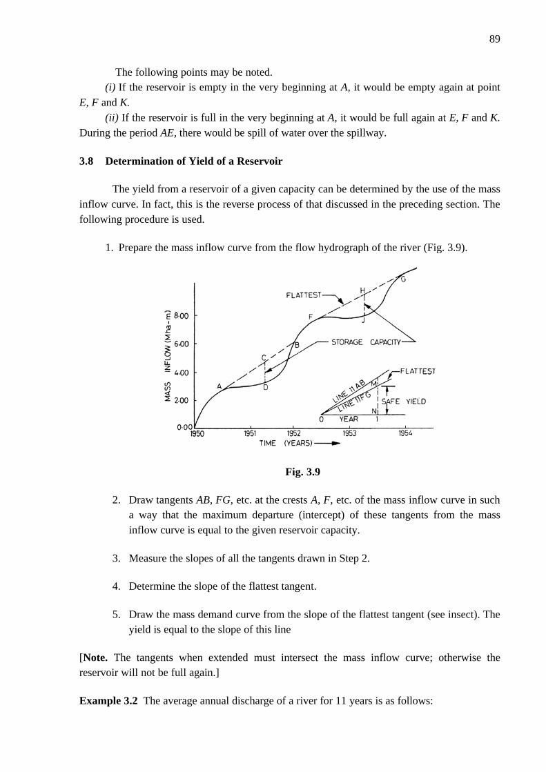
3.8 Determination of Yield of a Reservoir

The yield from a reservoir of a given capacity can be determined by the use of the mass inflow curve. In fact, this is the reverse process of that discussed in the preceding section. The following procedure is used.

1. Prepare the mass inflow curve from the flow hydrograph of the river (Fig. 3.9).

Fig. 3.9

2. Draw tangents AB, FG, etc. at the crests A, F, etc. of the mass inflow curve in such a way that the maximum departure (intercept) of these tangents from the mass inflow curve is equal to the given reservoir capacity.

3. Measure the slopes of all the tangents drawn in Step 2.

4. Determine the slope of the flattest tangent.

5. Draw the mass demand curve from the slope of the flattest tangent (see insect). The yield is equal to the slope of this line

[Note. The tangents when extended must intersect the mass inflow curve; otherwise the reservoir will not be full again.]

Example 3.2 The average annual discharge of a river for 11 years is as follows:

90

Year 1960 1961 1962 1963 1964 1965 1966 1967 1968 1969 1970 Discharge (cumecs)

1750 2650 3010 2240 2630 3200 1000 950 1200 4150 3500

Determine the storage capacity required to meet a demand of 2000 cumecs throughout the year. Solution 1 cumec- year = 1 x 365 x 24 x 60 x 60 = 31.536 x 106 m3 = 3153.6ha-m Yearly demand = 3153.6 x 2000 = 6.31 Mha-m Inflow volume in 1960 = 1750 x 3153.6 = 5.52 x 106 ha-m = 5.52 Mha-m

The inflow volume and cumulative inflow are calculated in the table below: Year 1960 1961 1962 1963 1964 1965 1966 1967 1968 1969 1970

Discharge (cumecs)

1750 2650 3010 2240 2630 3200 1000 950 1200 4150 3500

Inflow volume (Mha-m)

5.52 8.35 9.49 7.06 8.29 10.09 3.15 3.00 3.78 13.09 11.04

Cumulative inflow (Mha-m)

5.52 13.87 23.36 30.42 38.71 48.80 51.95 54.95 58.73 71.82 82.86

Fig. 3.10 shows the mass inflow curve. The tangents are drawn at the crests at the slope of 6.31 Mha-m per year. The maximum intercept is 7.7 Mha-m. Storage capacity = 7.7 Mha-m.

Fig. 3.10

3.9 Analytical Method for Determination of Storage Capacity

As discussed in the preceding section, the mass inflow, the storage capacity and the yield are interdependent. Because the inflow to a reservoir is variable and at times less than the demand, the storage reservoir is required. The storage capacity should be adequate to supply the water equal to the demand during the critical period. The greater the demand, the larger will be the storage required. However, for a long period, the total outflow volume from the reservoir must be equal to the total inflow volume minus the volume of water lost and wasted during the period. In other words, the reservoir does not produce water. It is a sort of water bank in which the total credit and total debit during the period are equal The capacity of the reservoir is determined from the net inflow and demand. The

91

storage is required when the demand exceeds the net inflow. The total storage required is equal to the sum of the storage required during the various periods. The following procedure is used for the determination of. storage capacity.

1. Collect the stream flow data at the reservoir site during the critical dry period. Generally, the monthly inflow rates are required. However, for very large reservoirs, the annual inflow rates may be used.

2. Ascertain the discharge to be released downstream to satisfy water rights or to honour the agreement between the states or the cities.

3. Determine the direct precipitation volume falling on the reservoir during the month.

4. Estimate the evaporation losses which would occur from the reservoir ‘The pan-evaporation data are normally used for the estimation of evaporation losses during the month.

5. Ascertain the demand during various months.

6. Determine the adjusted inflow during different months as follows:

Adjusted inflow = Stream inflow + Precipitation - Evaporation - Downstream

Discharge

7. Compute the storage capacity for each months. Storage required = Adjusted inflow - Demand

The storage would be required only in those months in which the demand is greater than the adjusted inflow.

8. Determine the total storage capacity of the reservoir by adding the storages required found in Step 7. Example 3.3 The monthly inflow and monthly pan-evaporation during a critical dry year at the site of a proposed reservoir are given below.

Month Jan Feb Mar April May June July Aug Sept. Oct. Nov. Dec. Inflow (ha-m)

10 10 4 2 1 200 2000 4000 1500 100 15 10

Pan evaporation (cm)

8 10 10 12 15 20 15 15 15 12 10 8

Precipita-tion (cm)

2 0 0 0 0 30 40 45 40 10 0 2

Demand (ha-m)

150 150 50 50 50 50 50 50 150 150 150 150

92

The net increase in pool area is 500 ha and the prior rights require the release of the full stream flow or 10 ha-m, whichever is less. Assume that 40% of the precipitation that has fallen on the submerged area reached the stream earlier and 60% of that directly falls on the reservoir. Determine the storage capacity. Take pan coefficient as 0.80.

Solution The solution is given in the tabulator form below.

Month 1

Inflow (ha-m)

2

Pan evaporation

(cm) 3

Precipitation (cm)

4

Demand (ha-m)

5

Water right

(ha-m) 6

Evapo-ration (ha-m)

7

Prect-pitation (ha-m)

8

Adjusted inflow (ha-m)

9

Required storage (ha-m)

10

Jan Feb March April May June July Aug Sept. Oct. Nov. Dec.

10 10 4 2 1

200 2000 4000 1500 100 15 10

8 10 10 12 15 20 15 15 15 12 10 8

2 0 0 0 0 30 40 45 40 10 0 2

150 150 50 50 50 50 50 50 150 150 150 150

10 10 4 2 1 10 10 10 10 10 10 10

32 40 40 48 60 80 60 60 60 48 40 32

6 0 0 0 0

90 120 135 120 30 0 6

-26 -40 -40 -48 -60 200 2050 4065 1550

72 -35 -26

-176 -190 -90 -98 -110

- - - -

-78 -185 -176

∑= -1103

Explanation Columns (1) to (6) are the given data

Column (7) = 100

8.0500)3( xxColumn= 4.0 x colm. (3)

Column (8) = 100

6.0500)4( xxColumn = 3.0 x colm. (4)

Column (9) = Columns (2) + (8) – (6) -(7) Column (10) = Columns (9) – Column (5), whenever negative Required capacity = total of column (10) = 1103 ha-m

3.10 Economic Height of Dam

Theoretically, economic height of dam is the height of dam corresponding to which the cost of dam per million cubic metre of storage is the minimum. This height of dam is determined by preparing approximate estimates of cost for several heights of dam at a given site, somewhat above and below the level, where the elevation storage curve shows a fairly high rate of increase of storage per metre of elevation; while at the corresponding elevation the cross section of the dam site shows the length of dam to be moderate, as shown in fig. 3.11 for a typical dam site.

93

Fig. 3.11

After thus determining the approximate cost per million cubic metre of storage for four or five alternative heights, the cost per million cubic metre of storage is plotted against height to assess the most economical height of dam as shown in fig. 3.12.

Fig. 3.12 Determination of economic height of dam

3.11 Reservoir Losses

The main losses are described hereinafter.

Evaporation Losses They depend on reservoir area and are expressed in cm of water depth. The other factors influencing evaporation are temperature, wind velocity, relative humidity, proximity of other structures etc. Evaporation losses can be measured on standard pans and after applying suitable coefficients, reservoir evaporation losses can be evaluated.

Cetyl alcohol is usually used for reducing evaporation losses in reservoirs. Cetyl alcohol, also called hexadecanol is a waxy substance made from sperm whale oil. When added to water, a mono-molecular layer is formed over the surface of water. The invisible film is non-toxic and retards evaporation, while allowing free passage of rain, oxygen and sunlight. The reduction in evaporation loss may be as high as 50 to 60 percent of natural evaporation. It is necessary to maintain the continuity of the cetyl alcohol film all the time.

94

Absorption Losses

They depend on the type of soil forming the reservoir basin. They may be quite large in the beginning, but gradually reduce as the pores get saturated.

Percolation or Seepage Losses

They are usually small but may be quite significant where there may be continuous seam of porous strata or cavernous or fissured rock.

3.12 Sedimentation in Reservoirs

Sedimentation in reservoirs is a difficult problem for which an economical solution has not yet been discovered, except by providing a “dead storage” to accommodate the deposits during the life of the darn. Disintegration, erosion, transportation, and sedimentation, are the different stages leading to silting of reservoir.

Mechanism of Sedimentation

In many respects deposits in a reservoir resemble those in a delta, made by a stream where it discharges into a lake or sea. These deposits are (i) bottom set beds, consisting of the fine sediments brought in by the stream, (ii) the fore set beds formed of the coarser sandy sediments (iii) top set beds consisting of coarser particles and (iv) density current deposits (Fig. 3.14).

Fig. 3.13

As a general rule, progressively small sizes of material will be deposited beyond the delta front, resulting in a gradual downward slope of the reservoir bed. It the stream carries an appreciable wash load, however, much of this material may not settle out as the cross-sectional area of the stream increases. Further more, the suspension may not mix completely with the clear water of the reservoir because of its difference in specific gravity. Instead a gravity underflow (more commonly but less appropriately known as a density current) may result

95

which will move through the entire length of the reservoir. Unless this portion of the flow is discharged at the dam, it will collect as a submerged pool, forming an almost level floor in the deepest part of the reservoir, where it will gradually compact.

The sedimentation is a product of erosion in the catchment area of the reservoir, and hence, lesser the rate of erosion the smaller is the sediment load entering the reservoir. Factors Affecting Sedimentation The following factors affect sedimentation

( i ) Extent of catchment area and the Unable nature of its different zones. ( ii ) Amount of sediment load in the rivers. (iii) Type of rainfall and snowfall in each zone. (iv ) Mean monthly and annual temperature in each zone. ( v ) Monthly and annual run-off from catchment or sub-catchment. (vi) Slope of each zone of catchment. (vii) Vegetation in each zone of catchment. (viii) Geological formations of each zone and estimated relative weathering and erosion

with due regard to climatic conditions. (ix) Presence of upstream reservoir and extent of trapping of sediment therein. (x) Amount of sediment flushed out through sluices. (xi) Degree of consolidation of the accumulated sediment depending upon the extent

of exposure to air, sun and wind. (xii) Volume of water in the reservoir and its proportion to the mean annual flow in the

river i.e. capacity inflow ratio. (xiii) Operation schedule of the reservoir.

Control of Silting of Reservoirs

The following are the three general means of controlling reservoir silting.

1. Adequate consideration of the silt factor for the selecting of site and design of the dam.

(a) Selection of reservoir site—If reservoirs of equal size could be constructed in either of the two watersheds at approximately the same cost, the watershed having less erosion should be preferred.

(b) Ratio of reservoir capacity and size of drainage area. It also affects the annual rate of storage depletion. According to Carl. B. Brown, of U.S. Deptt, of Agriculture, a reservoir should hold at least 3.6 hectare metre of water per square km of drainage area in order to have a safe life of 100 years.

2. A plan of water release designed to eject the maximum possible sediment load before deposition.

96

(a) Reservoir design —A lower darn in the first instance with provision in its structural design for its being raised in stages, as its capacity is encroached, would be a better proposition.

(b) In some of the reservoirs, sluices may be provided to take advantage of formation of density currents and thus eject a significant share of Sediment load.

(c) The reservoir may be filled, only after passing the peak flood-design of Aswan clam in Egypt provided for this.

3. Control of soil erosion and sediment movement in the catchments area.

(a) Control of sediment inflow —Small check dams may be constructed on all tributaries of the main river. Vegetation screen on the catchment would go a long way in reducing erosion.

(b) Control of sediment deposit—The outlets may be opened at the time when there is maximum inflow of sediment in the reservoir i.e. during monsoon periods; also ejection of reservoir water at lower levels would help in reducing silt in the basin.

(c) Removal of sediment deposit— Scouring, excavation, dredging etc. may be resorted to. But these methods are expensive. Loosening the sediment and or pushing it towards the sluices by mechanical means simultaneously with scouring would increase the effectiveness of the scouring action to some extent.

(d) Erosion control in the catchments area Soil conservation methods, like afforestation, control of grazing, terrace cultivation, provision of contour bunds, gully formation by providing small embankments, where necessary, debris barriers, weed growth etc. all help to control soil erosion and thus reduce sediment entry in the reservoir.

3.13 Life of a Reservoir

The dead storage provided in reservoir capacity is allowed for sedimentation. Actually all the sediment load does not go in dead storage. It encroaches upon live storage also. The encroachment and its distribution depend upon many factors such as reservoir operation, valley characteristics, capacity inflow ratio, sediment content in the inflow etc. The useful life of a reservoir is taken till its capacity is reduced to about 20% of’ the designed capacity.

The rate of sedimentation is higher in the initial stages and it decreases with years. This is due to fall in the trap efficiency of the reservoir, consolidation and shrinkage of deposits and formation of delta.

97

CHAPTER 4 GRAVITY DAMS

4.1 General A gravity dam derive its stability from the force of gravity of the materials in its section. The dead weight of the body of the dam and the manner of its distribution in the section is such so as to withstand the forces of water impounded in the lake behind it and other forces consequent there to. The first masonry dams were those built in Spain in the 16th and 17th centuries; they are about 20 m high, have a vertical upstream face and are approximately rectangular in section; in some cases the downstream face descends in steps. 4.2 Criteria for Selection of Dam Site A site for gravity dam is expected to satisfy the following requirements. (i) A narrow gorge at dam site, opening upstream. (ii) Sound rock able to resist static and dynamic forces including earthquakes. (iii) Stable valley and abutment slopes. (iv) Foundations having same value of elastic constants preferable. (v) The foundations and reservoir walls watertight, resistant to erosion, and other

detrimental effects of wetting, drying, freezing and thawing. (vi) Good location for spillways and power house. (vii) Availability of good construction material near by (viii) Proximity of construction facilities, like electric supply, road and rail

communications etc. 4.3 Foundation Treatment The purpose of the foundation treatment are : (i) to prepare stable support for the dam. (ii) to safeguard against uplift and water creeping through the junction of dam and

foundation, and (iii) to safeguard sliding. For this the processes used to treat the foundation zone, include : (a) Preparation of rock at dam interface. (b) Foundation grouting. (c) Treatment of faults, shear joints etc. (d) Drainage. These are briefly discussed below.

98

Preparation of rock and dam interface The foundation below the dam base is prepared some what as shown in figure 4.1.

Fig. 4.1 Preparation of rock below dam base Some engineers prefer location of shear key at the base centre, but these keys are usually given at the dam heel as shown. Foundation Grouting Foundation grouting mainly consists of the follow types Consolidation grouting The whole dam base area, is consolidated by 15 metres deep gout holes spaced about 3 to 6 metre depending on rock conditions. The grout pressures used are about 3.5 kg/cm2. In the execution of program, holes are drilled and grouted from 12 to 25 m apart before the intermediate holes are drilled. The upstream line of holes is upstream of heel of furnish a cut-off for leakage of grout from the high pressure holes used later in the same area. The holes are normal to surface except in cases where some seams are to be intersected. Curtain grouting High pressure holes are drilled relatively deep near the upstream face of the structure to form the principal grout curtain or seepage barrier (Fig. 4.2). Tentative spacing is 1.5 m centres. The holes are first drilled about 12 m c/c and then intermediate holes. In a hard rock the holes are drilled to depth equal to 30 to 40 p.c. of dam height (or water depth). In poor rocks deeper holes as much as 70 p.c. head may be drilled. The grouting is usually done in stages of about 15 m depth. The usual grout pressure is 0.25 kg/cm2 for each metre depth below the surface.

99

Fig. 4.2 Curtain grouting and drainage arrangements

Treatment of faults and shear joints etc If the exploratory drilling or the final excavation uncovers faults, seams etc, they are excavated and backfilled with good concrete to a depth sufficient to produce elastic qualities and bearing strength equal to that of the surrounding rock. R.S. Varshney after extensive photo elastic and computer studies found that the optimum depth of backfilling is 20 p.c of the height of the dam. U.S.B.R has given the following relations d = 0.0066 b.h + 1.5 for h > 46 m

d = 0.3 b + 1.5 for h < 46 m where

h = height of dam above general foundation level in metre b = width of weak zone in metre d = depth of excavation of weak zone below surface at adjoining sound rock in metre.

Drainage Although a well executed grouting program will materially reduce seepage; some means must be provided to intercept the water which will percolate through and around the grout curtain and which, if not removed, may cause high hydrostatic pressures on the base of structure. Drainage is accomplished by drilling one or more row of holes (N x size) to depths varying from 20 to 40 p.c. of hydrostatic head. The spacing is decided on the basis of judgment of the physical characteristics of rock. The drainage holes are made through a foundation gallery of usual size 1.8 x 2.2 metre at a distance of about 10 p.c. water depth from upstream face.

100

4.4 Joints and Keys Most concrete dams are sub-divided into a number of blocks to relieve the thermal stresses and subsequent cracking in the body of the dam. Transverse Joints For dams transverse joints normal to dam axis are given. These joints are 12 to 18 metre centres apart, usual spacing being 15 m. These joints are thus man made cracks (Fig.4.3) which allow the contraction of the concrete on the two sides to relieve thermal stresses. The edges of the transverse or contraction joint at the face are chamfered to give a pleasing appearance and to avoid spalling. Such chamfers are 4 x 4 cm on non-overflow blocks and 2 x 2 cm on the downstream face of overflow blocks. Longitudinal Joints As height of the dam increases, base thickness approaches a limiting dimension beyond which condition favorable to vertical cracking parallel to axis is created. To prevent uncontrolled cracks, longitudinal joints are provided. They serve the same purpose in one block of the dam as the transverse joints in the dam as a whole. Spacing of these joints vary from 15 to 50 metre (Fig. 4.3 ) . Where the longitudinal joints approach the downstream face of the dam, the joint is turned normal to the face to avoid feather-edging of concrete. A gap is often provided at the inclined portion of the joint which is later dry packed. Extension of longitudinal joints in the upstream face is undesirable; should be terminated at a minimum distance of 4-5 metre from the face. These joints are staggered in adjacent blocks. Construction Joints Concrete is placed in the dam in lifts which are generally 1.5 m high. To develop proper bond between the lifts, the lift surface is freed of all laitance, coatings, stains, defective concrete and all foreign material and the surface is roughened. Keys Provision of shear keys in joints enables transfer of stress from one block to the other through shear. These days such keys are given only in longitudinal joints as shown in fig. 13.5.

101

Fig. 4.3 Transverse and longitudinal joints

4.5 Cooling Arrangements

In concrete dams, cooling is mostly done by precooling the aggregates and placing the concrete in forms at sufficiently low temperatures. The placement temperature is fixed in such a manner as to result in a rise above the stable temperature less than what could cause cracking in the concrete. This cooling may be done either by precooling aggregates etc or by embedding thin walled tubing in concrete and passing water through these

4.6 Waterstops at Joints

The water stops are provided in transverse joints for stopping the flow of water into the joint and for stopping the flow of grout outside it. In longitudinal joints the only function of water stops or water seals is to retain the grout.

Fig. 4.5 Water stops

102

Usually copper (20 gauge) water stops are used. Recently monel (an alloy of nickel and copper) water stops are used. Stainless steel stops are also being used. Sometimes rubber and polyvinyl chloride water stops are also used. Some details of water stops are shown in figure 4.5 The usual practice is to provide two water stops of copper or monel with an asphalt seal in between. The longitudinal joints are provided with Z type while the transverse joints are provided with U or M type seals. Construction joints are sometimes provided with A or Z type seal to prevent seepage along the joint when some opening is located close to the face. The distance of the first seal from the upstream face in ungrouted contraction joints is about 0.6 metre. The pipes inside the asphalt well are installed for melting asphalt and adding more asphalt and adding more asphalt at a later period. Another metal seal is placed downstream of asphalt seal. The purpose of the seal is to limit the travel of asphalt along the joint in between the two seals. Further downstream, open drains (called formed drain) about 15 to 20 cm diameter at 3m centre to centre are provided.

4.7 Closing Gaps

Closing gaps are provided in between blocks for adverse conditions due to temperature effects, foundation requirements, unusual size of structure and in stage construction. These are called twist stats, shear slots or temperature control slots depending upon the purpose behind the provision. These are usually 1.5 metre or so in width or diameter. Twist slots at Grand Coulee dam were 1.81 metre wide and extended from the foundation to the top of dam.

4.3 Forces Acting on Dam

A gravity dam derives its stability from the force of gravity of the materials in its section, and hence the name. The gravity dam has sufficient weight so as to withstand the forces and the overturning moment caused by the water impounded in the lake behind it. It transfers the loads to the foundation by cantilever action and hence good foundations are prerequisite for the gravity dam. 1. Forces causing stability : (i) Weight of the dam, (ii) The thrust of the tail water. 2. Forces causing instability : (i) Reservoir water pressure, (ii) Uplift, (iii) Forces due to waves in the reservoir, (iv) Ice pressure, (v) Temperature stresses, (vi) Silt pressure, (vii) Seismic forces; (viii) Wind pressure.

103

Classification of loading for design Normal Loads They are those, under the combined action of which the dam shall have adequate stability, and the factors of safety and permissible stresses in the dam shall not be exceeded. Theses loads are : (i) Water pressure corresponding to full reservoir level. (ii) Weight of dam and structure above it. (iii) Uplift. Abnormal Loads These are the loads which in combination with normal loads encroach upon the factor of safety and increase the allowable stresses although remaining lower than the higher emergency stress limits. Such loads are : (i) Higher water pressure during floods, (ii) Wave pressure, (iii) Silt pressure, (iv) Ice thrust, (v) Earthquake force. Load Combinations Design should be based on the most adverse combination of 'probable' load conditions, but should include only those loads having reasonable probability of simultaneous occurrence U.S.B.R. specifies 'Normal' and 'Extreme' load combinations as below : Normal Load Combination (i) Normal design reservoir elevation with appropriate dead load, ice and silt (if applicable), and normal uplift. If temperature loads are applicable, minimum usual temperatures are to be used. Unusual load combination (i) Maximum reservoir elevation with appropriate dead load, silt (if applicable), normal uplift, minimum temperature if applicable and tail water. Extreme load combination (i) Normal design reservoir elevation with appropriate dead load, silt and ice (if applicable), uplift normal, minimum temperature if applicable, tail water and maximum credible earthquake.

104

Other studies (i) Maximum design reservoir elevation with appropriate dead loads, silt, minimum

temperature occurring at that time if applicable, tail water and uplift with drains inoperative.

(ii) Any of the above loading combinations for foundation stability. (iii) Any other loading combination considered desirable by the designer. Reservoir empty (i) Empty reservoir (without earthquake) should be computed for reinforcement

design, grouting studies, or other purposes. (ii) Construction stage-reservoir empty, earthquake considered, but no wind load. The Indian Standard Criteria (IS: 6512-1972) lay stress on the most adverse load

combination A, B, C, D, E, F and G as given below: (a) Load combination A (const. condition)-dam completed but no water in reservoir

and no tail water. (b) Load combination B (normal operating condition)- Full reservoir elevation,

normal dry weather tail water, normal uplift, ice and silt (if applicable). (c) Load combination C (Flood discharge condition) – Reservoir at maximum flood

pond elevation, all gates open, tail water at flood elevation, normal uplift and silt (if applicable).

(d) Load combination D – Combination A with earthquake. (e) Load combination E – Combination B with earthquake. (f) Load combination F – Combination C, but with extreme uplift. (g) Load combination G – Combination E, but with extreme uplift. 4.4 Types of Loads Weight of dam and appurtenant structure The weight of the dam and concrete structure over it, can be computed by taking unit weight of concrete as 2.4 t/m3. The computations of weight of dam should allow for the reduction due to openings of size larger than 1 metre. Smaller openings may be neglected for calculation of weight as well as stresses. The weight of the structures constructed on the dam should be estimated with fair amount of accuracy. These include the weight of gates, gantry on the top of dam and weight of towers at roadway level. The cross section of the dam may be divided into several triangles and rectangles and the weights W1, W2, W3 etc. of each of these may be conveniently computed along with their lines of action. The total weight W of the dam acts at the centre of gravity of the section. Water pressure on dam Water pressure on dams can be calculated by the law of hydrostatics, wherein the pressure at any depth 'h' is given by 'wh' t/sq m, acting normal to the surface. Where the dam has a sloping upstream face, the water pressure can be resolved into its horizontal and

105

vertical components; the vertical component being given by the weight of water prism on the upstream face and acts vertically downwards through the centre of gravity of the water area supported on the dam face. Referring to fig. 4.6 the total horizontal pressure (H) on a section of the dam per unit width is given by wh2/2 (in t); where w is unit weight of water = 1 t/m3 and h is height in m. The vertical weight Ww can be evaluated by the area of the trapezium and multiplied by w, the unit weight of water. The total pressure acts at a distance h/3 from the base of dam, hence the moment about base, in t.m = (wh3/6).

Fig. 4.6 Water thrust

In spillway sections, when the gate is closed, the water pressure can be worked out in same manner as for non-overflow section except for the vertical load of water on the dam itself. During overflow, the top portion of the pressure triangle gets truncated (Fig. 4.2) and a trapezium of pressure acts. If there is some negative pressure downstream of crest, it has to be added to this pressure.

Fig. 4.7 Water thrust on spillway

The pressure due to tail water is obtained in the same manner as for the upstream reservoir water. Silt load The weight and pressure of submerged silt is to be taken in addition to the water weight and pressure. The weight acts vertically on the slope and pressure horizontally exactly in the same way as the corresponding forces due to water.

106

The horizontal pressure due to silt load is taken as (0.36 h12/2) where h1 is the height to which the silt would be deposited. The combined horizontal pressure due to water and silt would therefore be 1.36 (h12/2). For calculating the vertical pressure, the density of the wet silt may be taken as 1.92 t/m3. Experimental and analytical procedures have both shown that an earthquake acceleration up to about 0.3 g is only about half as effective in silt or soil masses, as it is in water. This is due to the internal shear resistance of the soil. Since the unit weight of water is nearly half that of silt, the increase in silt pressure due to earthquake is ignored. Uplift Forces Recent trends for evaluating uplift forces is based on the phenomenon of seepage through permeable material. Water under pressure enters the pores and fissures of the foundation material and joints in the dam. The uplift is supposed to act on the whole width of the foundation. The pressure at heel is taken equal to whu where w is the unit weight of water and hu is the water head at the heel. On the downstream, the value is whd, where hd is the tail water depth at the toe. If there are no drainage galleries or if they are choked, the uplift is assumed to vary linearly from whu to whd (Fig. 4.8)

Fig. 4.8 Uplift pressure diagram – Drains choked (i) If drainage galleries are working, the reduction in water pressure head at the gallery is

taken as 3

2 rd of the difference between whu and whd or net pressure being whu -

3

2 (whu-whd),

(Fig. 4.9) It is assumed that the uplift pressure are not affected by earthquake forces because of their transitory nature.

Fig. 4.9 Uplift pressure diagram – Drains working

107

Seismic forces Seismic forces envisage the consideration of loads on the structure during an earthquake. The physical action of the earthquake is to rock the structures, which collapse when the shaking is severe. The intensity of an earthquake is measured on the basis of damage caused by it. The effect of an earthquake is to impart a momentary acceleration to earth crust in the direction in which the wave is

Table 4.1

Rating according to modified Mercalli’s scale Class of

earthquake Effects Ground

acceleration III VI VII IX X XII

Felt quite noticeably indoors; standing cars many rock slightly Felt by all, many frightened and run outdoors; a few instances of fallen plaster or damaged chimneys Everybody runs outdoors, damage negligible in buildings of good design and construction; some chimneys broken Damage considerable; framed structures thrown out of plumb; buildings shifted off foundations; ground cracked and underground pipes broken Some well built wooden structures destroyed; most masonry and framed structures with foundations destroyed; ground badly cracked; rails bent; land slides. Total damage; waves seen on ground surface, line of sight and level distorted; subjects thrown upward into the air.

0.005 g 0.05 g 0.1 g 0.5 g 1 g 5 g

traveling at that instant. The intensity scales, in terms of a friction of g, acceleration due to gravity, are based on the acceleration of vibratory motion. The rating, according to modified Mercalli scale is given in Table 4.1. The earthquake wave may travel at any inclination through the foundation; it is usual to consider a vertical and horizontal acceleration acting separately. Theoretical calculations indicate that the distribution of hydrodynamic pressure due to an earthquake on the upstream face of dam is nearly parabolic. The following formula of U.S.B.R (after C.N. Zanger) may be used to evaluate pressure intensity due to earthquake

Pe = C α w.h. (4.1) where Pe = Pressure intensity in t/m2

α = Horizontal seismic coefficient e.g o.1 in earthquake intensity of 0.1 g w = Unit weight of water = 1 t/m3 h = Maximum depth of reservoir in m C = A coefficient, given as below :

= 2

Cm [z/h (2-z/h) + )]2(/ hhz − (4.2)

108

where z = Depth in m from top of reservoir to the point under consideration Cm depends on upstream slope and

= 0.73

o90θ

(4.3)

θ = angle in degrees that the upstream slope of the dam makes with the horizontal. The total pressure Pe on the portion of the dam up to depth z from top is given by Pe = 0.726 Pe z. (4.4)

The moment Me about the plane upto which pressure is taken is given by Me = 0.3 Pe z2 (4.5) A horizontal acceleration towards the reservoir causes a momentary increase in water pressure as the foundation and dam accelerate towards the reservoir and the water resists the movement owing to its inertia. Thus the force is taken acting in the opposite direction of the earthquake acceleration. When the upstream face is partly vertical and partly sloping two cases arise. (i) When the vertical portion is more than half the depth; the entire face is taken vertical/ (ii) When the vertical portion is less than half the depth; the slope of the face is given by the line joining the heel to the water surface level at the upstream face. Effect of Vertical Earthquake Acceleration On account of earthquake the gravity acceleration is increased or decreased according to the direction of earthquake tremor thereby affecting the weight of both masonry and water in the same proportion. The increase in gravity acceleration in down ward direction therefore causes increase in weights of both the dam and the water and they have to be multiplied by (1+αv) while decrease in gravity acceleration, which results due to upward movement causes decrease of weight which have then to be multiplied by (1-αv). [αv = vertical earthquake acceleration coefficient]. Consequently, stresses may be computed directly from stresses for normal conditions. However the effect on horizontal water and silt pressure may be neglected for small and medium dams (C.W.C Criterion). Thus the net effect of the vertical earthquake acceleration may be summarized as below : 1. On sloping faces of the dam the weight of the water above the slope should be modified by the appropriate acceleration factor. 2. The unit weight of the concrete should also be modified by this acceleration factor. 3. For high and important dams, the components of water pressure normal to the upstream face of the dam is modified by the given acceleration factor i.e. taken as 1 +αv or 1-αv

times the normal pressure. Effect of Earthquake on Spillways The fact that the water flowing over the spillway crest is not restrained may probably reduce the earthquake force below the crest as well. Creager and Justin have given force and moments for such cases in terms of percentage of force and moment on non-overflow sections. If He and h represent the head of water above the spillway crest and

109

the total depth of water respectively, the percentages of force and moments due to earthquake may be taken as given in Table 4.2 Resonance The consideration of seismic loads on gravity dams have two aspects-effect of vibration on the body of the dam and the effect on water pressure. As far as the effect on the dam are concerned the problem centres around finding a suitable acceleration for design. Secondly it has got to be assured that the natural period of vibration of the dam does

Table 4.2 Recommended reduced values of pressures and moments

Ratio He / h Percentage of force Percentage of moment 1.0 0.8 0.6 0.4 0.2 0.0

0.0 29.0 53.0 74.4 90.0 100.0

0.0 8.0 26.0 53.0 80.0 100.0

not coincide with the period of earthquake. The period of vibration of gravity dams is calculated by Westerguard formula

T = b

h610

2 (4.6)

where h = height of the dam in m b = base width of dam in m T = period of vibration in secs. The period of vibration of gravity dams is very low while the least period of vibration of an earthquake is 1 second. Force due to waves Wind blowing over the reservoir area causes a drag on the surface. The effect of the drag is to pull the surface along the direction of wind and thus ripples and waves are formed. The following formulae given by Molitor Stevenson may be used to evaluate the height of waves.

hw = 0.032 FV . + 0.763 – 0.27 4 F (4.7) for F < 32 km, and

110

hw = 0.032 FV . for F > 32 km (4.8) where hw = height of waves in metre V = wind velocity in km per hour F = fetch or the straight length of expanse in km The pressure intensity due to waves is given by the formula (in t/m2) Pw = 2.4 w.hw (4.9)

The total pressure is given by the relation (in t) Pw = 2.0 w.hw

2 (4.10) and the moment (in t.m) can be found with respect to the centroid of the pressure diagram (Fig. 4.10) which is 3 hw/8 above reservoir level.

Fig. 4.10 Wave pressure – Wave diagram Wind Pressure In designing a dam section, wind pressure is generally not considered. It may be taken as 100 to 150 kg/m2 for the area exposed to the wind pressure. Force due to Temperature Variation The forces caused due to variation in temperature are of secondary importance in gravity dams since these only case secondary stresses.

111

4.5 Safety Criteria Safety against Overturning If the resultant of all the forces acting on a dam passes outside the base, the dam would overturn unless it can resist tensile stresses. Since the dam is usually designed on no tension basis, it follows that the resultant should pass through the middle third. If other safety criteria like maximum compressive stresses and sliding are also fulfilled, then usually a factor of safety between 1.5 to 2.5 is available against overturning. Factor of safety against overturning may be defined as the ratio of the stabilizing moments to the overturning moments about the toe of the dam. Safety against Sliding In order that the dam may not slide on any plane, the total forces tending to slide the dam should not exceed a certain ratio of the normal force on the plane. Expressing mathematically ΣH/ΣV < f, where f is the coefficient of friction. The safe value of 'f' is usually taken up to 0.75. In certain cases this value, under abnormal loading conditions, becomes more than 0.75. When 'f, becomes more than 0.75, the shear friction factor may be calculated.

S.F.F = H

AsrVfΣ+Σ ..

(4.11)

where f = 0.7 s = shearing strength which varies from 140 t/m2 for poor rocks to 500 t/m2 for good rocks. r = averaging factor = usually 0.5 A = area in m2 As per U.S.B.R. recommendation the value of shear friction factor should not be allowed to go below 5 under normal loading, and in abnormal loading conditions it may be encroached upto 4. However uneconomical sections of dam result with this criterion when dam height exceeds 150 m. It is recommended that for dams higher than 150m, these factors be taken as 4 for normal loading and 3 for extreme loading conditions. I.S.S (6512-1972) recommend the following shear friction factors.

Table 4.3 Factors of safety against sliding and S.F.F.

Loading condition as per I.S.S S.F.F 1. A,B,C 2. D,E 3. F,G

4.0 3.0 1.5

112

Safe Stresses The stresses in the dam should be within the specified limits for the body of the dam and in the foundations. If the stresses at the toe and heel are excessive, they can be brought within permissible limits with the provision of fillets. The height of these fillets above the heel and toe are given by the following relations. For heal

hf = 6H - 52.1

2H - 1.07

where H = height of dam in 100 metre and hf = height of fillet in metre For toe hf = 6.5 H – 1.1 H2 – 0.9 Usually sloping fillets with 2 horizontal to 1 vertical at downstream and 1 horizontal to 2 vertical on the upstream are provided. Tensile stresses should not be higher than 5 kg/cm2 for height concrete dams under the most adverse loading conditions, with gravity analysis. In case of elastic analysis of dam say with finite element method of design, very high tensile stresses are obtained at the heel. In such cases the dam should be analyzed again with an assumed crack in the rock mass in the heel region. If tension is eliminated by assumption of crack, the dam may be considered safe. The cracking, due to tension, reduces the joint area for distribution of stresses and hence increase the compressive stresses at the toe. Failure would ultimately take place when the toe is crushed. The maximum permissible compressive stress in a dam depends on the crushing strength of concrete, which is usually between 150 to 300 kg/cm2. A factor of safety of 3 to 4 is considered adequate for determining the stresses. In case of unusual loading conditions, U.S.B.R. recommends lowering of safety factor to 2 and allowable compressive stress 100 kg/cm2. In extreme loading condition U.S.B.R. allows safety factor of even 1.0. 4.6 Gravity Analysis 1. Assumptions in the design The dam is considered to be made up of a number of vertical cantilevers which act independently of each other. The following assumptions for the gravity analysis are made (i) The material in the foundation and in the body of dam is isotropic and

homogeneous. (ii) The stresses in the foundation and the body of the dam are within elastic limits. (iii) No movements are caused in the foundations due to transference of the load. (iv) The foundation and the dam behave as one unit, the joint being a perfect one. (v) No loads are transferred to the abutments by beam action.

113

(vi) The stability analysis of the dam is based on considering a slice of the dam one metre thick at the base line and contained between the two vertical planes normal to the base line.

(vii) Small openings are supposed to have a local effect only and according to St. Venant's principle, the openings would not affect the general distribution.

Stresses at the Upstream and Downstream Ends The direction of axes, notations of forces etc. are exhibited in figure 4.11 σz = Vertical normal stress on horizontal planes. σy = Horizontal normal stress on vertical plan

τyz = τzy = Shear stress.

Fig. 4.11 Forces and moments sign-conventions (Gravity analysis)

The origin of coordinates is always taken at the downstream end of the horizontal plane. The distribution of σz is σz = a + by (4.14) By equating vertical loads and moments about the centre of gravity of the horizontal section we have

a = 2

6TM

TW

− and b = 3

12T

M (4.5)

114

where W is total vertical load in t M is total moment in t.m. about centre of gravity, and T is width of section in m.

If the resultant of forces acts at a distance 'e' from the centre of the area, then intensities of stresses at the toe and heel are given by the relation,

)/61( TeTW

z ±=σ (4.16)

4.12 Elementary Profile of a Gravity Dam If we consider only hydrostatic force, the elementary profile will be triangular in section (Fig. 4.12), having zero width at the water level; where water pressure is zero, and a maximum vase width b, where the maximum water pressure acts. Thus the section of the elementary profile is similar to the shape of hydrostatic pressure distribution diagram. The same profile will provide the maximum possible stabilizing force against overturning, without causing tension at the base. If any other triangular profile, other than right angled one is provided, its weight will act closer to the upstream face, which will cause tension at the toe. In the triangular profile the resultant, in case of empty reservoir condition, the gravity load only acts at a distance of b/3 from the heel i.e. at the extreme upstream middle third point.

Fig. 4.12 Gravity dam – elementary profile Minimum base width required for elementary profile under different design conditions (i) Dam safe against overturning, (no uplift) Taking moments about toe. (Fig. 4.12)

Moment of W about toe =w mh mh w m hc. 2 2 3

22

3 3=

Moment of H about toe = w h. 3

6

For safety

115

w m h w hc . 2 3 3

3 6- ≥ 0 or m =

cWw

2 ≥ 0.456

(we = 2.4 t/m3; w = 1 t/m3) i.e b ≥ 0.456 h (ii) Dam safe against overturning (uplift considered triangular distribution) From figure 4.12, we have for stability

w m h w h w m hc

2 3 3 2 3

3 6 3- -

.≥ 0

or m > w

w wc2( )-≥ 0.595 i.e. b ≥ 0.595.h.

(iii) Dam safe against overturning (uplift considered full uplift of intensity wh on full base

width) We have

w m h w h w m h

c2 3 3 2 2

3 6 2- - ≥ 0

or m ≥ w

w wc2 3-≥0.748 i.e. b ≥ 0.748h

(iv) Dam safe against sliding (uplift not considered) From safety considerations

HW

< f ≤ 0.75 say

or

w h

w mhc

2

22

2

≤ 0.75

or m ≥ 4

3ww c

≥ 0.555 i.e. b ≥ 0.555 h

(v) Dam safe in sliding (uplift considered - triangular distribution) As per given condition, from fig. 4.12

H

W U- ≤ f ≤ 0.75

or

w h

w mh w m hc

2

2 2

2

2 2-

.≤ 0.75

or m ≥ 4

3w

w wc( )-≥ 0.952 i.e. b ≥ 0.952 h

(vi) No tension in the dam (uplift not considered) Stresses due to gravity loads only

116

σz u = Wb

(1 + 6eb

) = Wb

(1 + 6

6b

b ) =

2wb

= 2

2w h b

bc . ..

= wc. h

τz u = 0

Stresses due to w h. 3

6 (moment due to water thrust)

σz u = - w h

b. 3

266

= - w hm h

3

2 2 = - w hm2

σz D = w hm2

Hence, by combining the two values

σz u = wc. h - w hm.

2

For no tension

wc. h ≥ w hm2 or m ≥

ww c

≥ 0.645

(vii) Vertical compressive stress at each level should exceed the water pressure at that point, for allowing uplift (Mauric Levy’s criterion): This means that (from condition vi)

h( wc - wm 2 ) ≥ wh

or m ≥ w

w wc -≥ 0.845 i.e. an increase of about 31 p.c. over the criterion vi.

(viii) Dam safe for no tension with triangular uplift considered Considering figure 4.12 and criterion 6,the effect of uplift is to reduce compressive stress at heel due to gravity load. The new compressive stress will now be (wc -w) h. For no tension condition

(wc - w) h ≥ w hm2 or m ≥

ww wc -

≥ 0.845 ie the same by criterion as given Levy.

4.13 Top Width And Free-Board The top width of a gravity dam is generally fixed by the provision of a road-way and side walls. The economical top width of a dam is about 14% of the height of dam. The usual widths provided vary from 6 to 10 metres. The free board in the dam should be ample to avoid overtopping of the dam during maximum flood coupled with waves. Usually a free - board of 1.5 hw (hw is the height of wave calculated by the equation 13.8 or 13.9) is given. The economical free-board is approximately 5% of the height of the dam.

117

4.14 Design Of Gravity Dam I DESIGN OF NON - OVERFLOW SECTION Design Example 4.1 Design the non- overflow section of a gravity dam with the following data: ( i ) R. L. of deepest foundation level 100 m ( ii ) R. L. of roadway at the top of dam 161 m ( iii ) Maximum pond level 152 m ( iv ) Maximum tail water level 123.9 m ( v ) Location of centre of drainage gallery form u.s. face of dam 7 m ( vi ) Roadway width at the top 6.1 m ( vii ) Downstream vertical face up to EI. 154.28 m (viii) Upstream face of dam vertical ( ix ) Downstream face of dam 0.9 horizontal to 1.0 vertical ( x ) Density of silt laden water 1.36 t/m3 ( xi ) Weight of concrete 2.4 t/m3 ( xii ) Safe bearing capacity 15 kg/cm2 (xiii) Shearing resistance of concrete (average) 21 kg/ cm2 (xiv) Minimum allowable shear friction factor under ( i ) normal loading = 5.0 ( ii ) abnormal loading = 4.0 ( xv ) Maximum coefficient of sliding under normal loading = 0.75 ( xvi ) Horizontal seismic coefficient = 0.20 g ( xvii ) Vertical seismic coefficient = 0.10 g Design A. Selection of Dam Profile The preliminary dam section is chosen on the basis of existing dam section of similar height. Usually upstream face is vertical and downstream slope varies from 0.9 to horizontal to 1.0 vertical; the flatter slope being given when earthquake forces are acting on the dam and extra section is required. The base widths derived in section 4.12 may be taken as a guide. The position of the foundation gallery is about 0.1 H, where H is the dam height, from upstream face. In this case, a gallery at a distance of 7 m been provided. The top width of the dam is provided for the roadway and is usually taken 6 to 9m. In the present case, the dam is medium high and hence top width is taken 6.1 m only. Since the earthquake forces are very high in the problem, the downstream face slope is assumed as 0.9 horizontal to 1 vertical. The upstream face has been chosen as vertical in this case. There would however, be no difficulty in solving the problem if the upstream face is sloping in full or is partly sloping. B. Steps in the Stability Analysis

1. Determination of forces and their moments All the force acting on the dam should be written first. For earthquake, the direction of acceleration should be mentioned, so as to determine the force correctly.

118

All the forces are calculated as per criteria and formulae detailed earlier. The moments are taken with respect to upstream heel point, for facility of calculations. In the example, for which data is given, the different loads have been calculated as below: (a) Dead weights The weight of the dam section can be found by dividing the section into simpler geometrical shapes, like triangle, rectangle, trapezium etc. The area of each part can be easily calculated and multiplying by density of concrete as 2.4 t /m 3, the weight of each part can be calculated. This weight acts vertically downwards through the center of gravity which can be found easily for each geometrical figure. Thus the weight W1 in the dam section pertains to the top triangle of width 6.1 m and height 6.72 m (width of dam section normal to the plane of

figure is taken as 1.0 metre) . The weight is given by 2 4 61 6 72

2. . .x x

i.e. 49 tons, acting at a

distance 2 /3 X 6.1 = 4.06m from upstream heel is therefore 49x 4.16 = 198 tm. We consider all clockwise moments about heel. The moment of this weight W1 about heel as negative and all anticlockwise moments as positive. Thus the moment due to all dead weights are negative. (b) Water Thrust The water pressure acts horizontally on the upstream face and is given by ½w. h2 . In this case, water thrust = ½ x 52 x 52x 1 = 1350 t . It acts at a distance of h /3 i.e 52 /3 m from heel. Hence moment is negative and equals to 1350 x 52 /3 = - 23400 t.m. (c) Uplift forces The uplift intensity at the upstream heel end is wh i.e. 52 t /sq. m and on the downstream it will be whd if hd is the tail water depth . In this case, tail water is taken as zero and hence uplift varies linearly from 52 t / sq m to 0 value at toe (when drains are choked). If drains are working then the balance uplift at the position of drain is 52/3 i.e 17.33t. The uplift pressure diagram can be conveniently divided into triangles and rectangles and the uplift pressure on the whole base width may be calculated similar to dead loads. The uplift on any portion will act from the centre of gravity of that part. Obviously these force are acting opposite to dead weight and are therefore, taken as negative. The moments about heel are anticlockwise and are therefore, taken as negative. The moments about heel anticlockwise and hence positive. (d) Hydrodynamic Pressure due to earthquake The horizontal earthquake will produce a force given by Pe = 0.726 Pe. h., where Pe = C a w h

= (0.73 9090

o

o ) 0.20 x 1 x 52 (for base)

(Since α = 0.20 and upstream face is vertical) ∴ P = 0.726 x 0.73 x 0.20 x 52 x 52 = 286 t The moment about heel is given by 0.3 peh2 = -0.3 x 0.73 x 0.20 x 523 = -6150 t.m.

It the earthquake acceleration is acting upstream the force is acting horizontally downstream and moment is negative and vice versa.

119

(e) Inertial forces due to earthquake (i) Effect of horizontal earthquake It will create acceleration in the dam body and consequently an inertial force which is dead weight of masonry multiplied by the earthquake coefficient α, is created. This force acts horizontally upstream or downstream depending on the acceleration direction of the earthquake), through the centre of gravity of the dam section. Its moment can be taken about the heel. (ii) Effect of vertical earthquake This will effect the inertial forces of the concrete mass and water. The forces will increase, if the earthquake acceleration is acting vertically up and decrease if the acceleration is acting downward. Thus the dead weighs and water pressure will be modified accordingly by multiplying forces and moments due to masonry and water by (1±αv) where αv is the vertical earthquake coefficient.

(f) Silt load The effect of silt of horizontal pressure is to consider the density of water as 1.36 t/m3, instead of 1 t/m3. If horizontal water thrust has been already considered, an additional thrust due to 0.36 t/m3 may be added i.e. 1/2 x 0.36 x 52 x 52 = 486 t in the present case. It acts at 1/3 h from heel i.e. 52/3 m from base giving a moment of -8450 t.m. Since upstream face of dam is vertical, no vertical silt load has been considered.

(g) Wave pressure The total pressure due to waves is given by 2.0 w hw

2. Since hw is given 1.5m in this case, P = 2.0 x 1.52 = 4.5 tons. (If reservoir 'fetch' and wind velocity are known, hw may be calculated from Molitor's formulae).

Since the pressure due to waves acts at height of (3 hw/8) = 3 1 58

× . = 0.6 m from

reservoir surface, lever arm of the pressure about upstream heel = 52 + 0.6 = 52.6 m. The moment about heel is negative and is equal to 4.5 x 52.6 = 236 t.m.

(2) Tabulation of Forces and MomentsHaving determined forces and moments, they can be tabulated and summed up. Dividing total moments (algebraic addition of positive and negative moments) by the total vertical force, the point of application of the resultant on the dam bottom line from heel is determined. Subtracting half bottom width from the above, the eccentricity of the resultant force is found.

(3) Determination of Stresses The stresses, σz and principal stresses σp on the upstream and downstream faces can be calculated from the formulae. The calculations for each case for the problem are given at the end of each table. Stress Analysis Case I. (Figure 4.13) (i) Reservoir full

Fig. 4.13 Non-overflow profile-design problem

120

(ii) No tail water (iii) Uplift considered (iv) Drains working (v) Horizontal earthquake acceleration upstream (vi) Vertical earthquake acceleration downward Line No.

Item Calculations Vertical force t

Horizontal force t

Lever arm m

Moments t.m.

- + 1 2 3 4 5 6 7 8

Weights

1. W1 61 6 72

22 4

. ..

× ×× 49 4.06 198

2. W2 61 54 9

22 4

. ..

× ×× 4,020 18.3 73,600

Inertial force due to earthquake 3. PeV (W1 + W2) (W1 + W2) x 0.1 - 407 7,380 4. Peh W1 (W1 x 0.2) 10 58.76 588 5. Peh W2 W2 x 0.2 804 61/3 16,300 Water Thrust 6. Pw 1/2 x 52 x 52 1350 52/3 23,400 Inertial effect due to vertical earthquake 7. Pwev -135 52/3 2340 Hydrodynamic force 8. Peh Pw Pe = 0.726 6,159 0.73 x 0.20 x 286 52 x 52 Me = 0.3 x 0.73 0.20 x 523 Uplift forces 9. U1 1/2 x 7 x 34.67 - 121 7/3 282 10. U2 7 x 17.33 - 121 3.5 423 11. U3 1/2 x 47.9 x 17.33 - 415 23 9,550 Total 4069 120245 19975 -1064 2315 Net = 100270 t.m. = 3,005 t Eccentricity = 33.1 - 27.5 = 5.6 m Vertical stresses

σz = ∑

±∑W

TW 6.eT2

= 300554 9

3005 6 5654 9 54 9.

.. .

±× ××

= 54.7 ± 33.4 σzD = 88.1 t/m2 = 8.81 kg/cm2 (compression) σzU = 21.3 t/m2 = 2.13 kg/cm2 (compression)

Principal stresses σp = σz sec2 φ

121

Since upstream face is vertical and there is no tail water σpU = 2.13 kg/cm2 σpD = ( 1+0.92) x 8.81 = 1.81 x 8.81 = 15.9 kg/cm2

Coefficient of sliding = ΣΣ

HW

=23153005

= 0.77

(on the higher side) Check for shear friction factor

= 3005 0 7 54 9 210

231513 6452315

59× + ×

= =. . ,

. Okay

Case II (i) Reservoir full (ii) No tail water (iii) Uplift considered (iv) Drains working

(v) Horizontal earthquake acceleration acting upstream and vertical acceleration acting up. (vi) Silt considered

Line no.

Item Calculations Vertical force t

Horizontal force t

Lever arm m

Moments tm

- + 1. W1 49 4.06 198 2. W2 4,020 18.3 73,600 3. Pev (W1 + W2) +407 7,380 4. Peh W1 10 58.76 588 5. Peh W2 804 61/3 16,300 6. Pw 1,350 52/3 23,400 7. Pwev 135 52/3 2,340 8. Peh Pw 286 7/3 6,150 9. U1 -121 7/3 282 10. U2 -121 3.5 423 11. U3 -415 23 9,550 12. Silt 1/2 x 0.36 x 486 8,450 Total 4476-657 3,071 33.7 138,406 10,255 =3819 -128,151 Eccentricity = 33.7 -27.5 = 6.2 m

σz = 381954 9

3819 6 6 254 9 54 9.

.. .

±× ××

= 69.5 ± 47.0

σzD = 126.5 t/m2 = 11.7 kg/ cm2 (compression) σzU = 22.5 t/m2 = 2.2 kg/ cm2 (compression)

principal stresses Since upstream force is vertical and there is no tail water

σpD = 1.81 x 11.7 = 21.2 kg/cm2 σpU = 2.3 kg/cm2.

122

Coefficient of sliding =30713819

= 0.805

Shear friction factor = 3819 0 7 210 54 9

3071× + ×. .

= 4.6 safe

Case III (i) Reservoir full up to 152 elevation (ii) No tail water (iii) Uplift considered (iv) Drains working (v) Horizontal earthquake acceleration acting upstream and vertical acceleration action

up (vi) Wave's force considered (hw = 1.5 m) Line No.

Item Calculations

Vertical force t

Horizontal force t

Lever arm m

Moments t.m.

- + 1. W1 49 4.06 198 2. W2 4020 18.3 73,600 3. Pev (W1 +

W2) 407 7,380

4. Peh W1 10 58.76 588 5. Peh W2 804 61/3 16,300 6. Pw 1350 52/3 23,400 7. Pwev 135 2,340 8. deh Pw 286 6,150 9. U1 -121 7/3 282 10. U2 -121 3/5 423 11. U3 -415 23 9,550 12. Pwaves 2 x hw

2

4.5 52.6 236

Total = 2x2.25 4476 130192 10255 -657 2589.5 31.5 = 3819t. = -119,937 t.m. Eccentricity = 31.5 – 27.5 = 4.0 m

σz = 4.305.699.549.54

0.4638199.54

3819±=

×××

±

σzD =99.9 t/m2 = 10.0 kg/ cm2 (compression) σzU = 39.1 t/m2 = 3.9 kg/ cm2 (compression) Principal stresses Since upstream face is vertical and there is no tail water σzD = 10.0 x 1.81 = 18.1 kg/cm2 σpU = 3.9 kg/ cm2

Coefficient of sliding = 2589 23819

.= 0.68

Shear friction factor = 3819 0 7 210 54 9

2589 5× + ×. .

.= 5.5 safe

123

Case IV (i) Reservoir upto EI. 152 m (ii) Drains chocked (iii) No earthquake Line No.

Item Calcula tions

Vertical force t

Horizontal force t

Lever arm m Moments t.m.

- + 1. W1 49 4.06 198 2. W2 4020 18.30 73,600 3. Pw 1350 17.33 23,400 4. U1 ½ x 52 -1430 18.30 26100

x 54.9 4069 Total -1430 1350 27 97,198 26,100 =2639 =-71098 tm Eccentricity = 27 – 27.5 = - 0.5 m

σz = 6.2489.549.54

5.0626399.54

2639mm =

×××

σzD = 45.4 t/m2 = 4.5 kg/cm2 σzU = 50.6 t/m2 = 5.1 kg/cm2 Principal stresses Since there is no tail water and upstream face is vertical σzD = 1.81 x 4.5 = 8.2 kg/cm2 σzU = 5.1 kg/cm2

Coefficient of sliding = 51.026391350

= safe

Case V (i) Reservoir Empty (ii) No earthquake Line No.

Item Vertical force t

Horizontal force t

Lever arm m Moments t.m.

- + 1. W1 49 4.06 198 2. W2 4020 18.3 73,600

Total 4069 18.15 m 73798 t.m. Eccentricity = 18.15 - 27.5 = - 9.35 m

σz = 406954 9

4069 6 9 3554 9 54 9

74 0 768.

.. .

. .±× ×

+= ±

σzD = - 2.8 t/m2 = -0.28 kg/ cm2 (minor tension, allowed) σzU = 150.8 t/m2 = 15.1 kg/ cm2 (compression)

The tentative section chosen for stability analysis is, therefore, suitable.

124

II Design of Overflow Section Design Example 4.2 Design the overflow section of a dam with the following data: (i) Bottom elevation of spillway section 100.0 m (ii) Crest elevation of spillway 136.6 m (iii) Upstream flood level 157.7 m (iv) Downstream tail water level 123.9 m (v) Downstream slope 0.9 : 1 (vi) Spillway width at foundation level 52.2 m (vii) Drains from upstream face 7 m (viii) Total weights as enumerated below 2820 t (ix) B.M. of the weight as in item (viii) 50300 t.m about heel Calculate stability (Fig. 4.14) (i) Drains are working (ii) No earthquake acting

Weights to be taken in design 1. Weight of concrete spillway 2. Proportional weight of pier 3. Proportional weight of gates and hoists 4. Weight of bridge 5. Weight of water over the crest. Line No.

Item Calculations Vertical force t

Horizontal force t

Lever arm m

Moments t.m.

- + 1 W all weight due to

concrete, gates, piers and water over crest etc.

2820 50,300

2 Wt 1/2 x 23.9 x 21.5 257 45.00 11,540 3 Pw1 21.1 x 36.6 773 18.30 14,100 4 Pw2 1/2 x 36.6 x 36.6 670 12.20 8,170 5 Pwt 1/2 x 23.9 x 23.9 -286 8.00 2,288 6 U1 1/2 x 7 x 22.5 -79 2.33 184 7 U2 35.2 x 7 -246 3.50 863 8 U3 1/2 x 11.3 x 45.2 -258 22.10 5,700 9 U4 23.9 x 45.2 -1080 29.60 22,000 3077 Total -1663 1157 30.5 84,110 41,035 = 1414 Net = - 43,075 t.m

125

Fig. 4.14 Spillway Profile - Design Example 4.2 Eccentricity = 30.5 - 26.1 = 4.4 m Vertical stresses

σz = 141452 2

1414 6 4 452 2 52 2

27 2 13 7.

.. .

. .±× ×+

= ±

σzD = 40.9 t/m2 = 4.1 kg/ cm2 σzU = 13.5 t/m2 = 1.4 kg/ cm2

Principal stresses Since upstream face is vertical σpU = 1.4 kg/cm2 Since there is tail downstream σpD = σzD sec2 φD - w.h. tan2 φD

= 4.1 x.1.81 - 2.39 x 0.81 = 7.4 - 1.93 = 5.50 kg/cm2

Coefficient of sliding = 11571414

= 0.82

Shear friction factor = 1414 0 7 210 52 2

1157× + ×. .

= 990 10950

1157+

= 10.3 safe

126

GALLERIES General

Galleries are provided in a dam for different purposes viz. grouting and drainage, operation of gates and control equipment, housing hoisting pumping and other equipment for measurement of structural behavior of the dam. In addition there can be other types of openings like sluices, conduits etc. Which run full of water. Thus we can divide galleries (i.e.a formed opening in a dam) as (i) hydraulic like sluices, outlets, penstocks etc. and (ii) galleries which can be termed as control and inspection passages. Galleries can be further subdivided according to their alignment viz. (i) Parallel to the axis of dam In this category, we can include: (a) Foundation and drainage gallery This gallery generally extends the length of the dam near the rock surface, conforming in elevation to the transverse profile of the canyon; in plan it is near to the axis of dam . It is from this gallery that the holes for the main grout curtain are drilled and grouted and also from which foundation drain holes are drilled. Its size is approximately 1.5 x 2.2 or 1.8 x 2.4 m. (b) Drainage Gallery A supplementary drainage is sometimes located further downstream, about 2 / 3rd of the base width from the upstream face, for the purpose of drilling and draining the downstream portion of the foundation. This gallery usually extends only through the deepest portion of the dam. (c) Gate Gallery Location and size depends on the need and size of the equipment to be housed. It usually connects hoisting chambers just over the control gates. Examples may be sluice-operating gallery, penstock-operating gallery etc. (d ) Grouting Galleries If it is difficult to grout contraction joints from the face of the dam the grout piping system should be arranged so as to locate the supply, return and vent headers in galleries placed near the top of each 15m life of concrete. The piping system for artificial cooling of the blocks should also be arranged to terminate in these galleries. (e) Inspection Galleries Sometimes some galleries are provided for inspection purposes.

(ii) Normal to dam axis In this group we can include adits, which are approaches to the different galleries. These adits also sometimes locate measuring boards of the different equipment's pump etc. (in recessed chambers)

(iii) Vertical and Inclined shafts These include: (a) Shafts for housing elevators, plumb bob etc. (b) Inclined shaft to connect two galleries or one gallery at two elevations.