chapter 3 - distillation column design
DESCRIPTION
Distillation column design in chemical industryTRANSCRIPT

3-1
CHAPTER 3
DESIGN FOR DISTILLATION COLUMN
3.1 INTRODUCTION
Distillation is most probably is the widely used separation process in the chemical industries.
The design of a distillation column can be divided into several procedures:
1. Specify the degree of separation required: set product specification
2. Select the operation conditions: batch or continuous: operating pressure
3. Select the type of contacting device: plate or packing
4. Determine the stage and reflux requirements: the number of equilibrium stages
5. Size the column: diameter, number or real stages
6. Design the column internals: plates, distributors, packing supports
7. Mechanical design: vessel and internal packing
The separation of liquid mixtures by distillation is depends on the differences in the volatility
between the components. This is known as continuous distillation. Vapor flows up to column
and liquid counter-currently down the column. The vapor and liquid are brought into contact on
plates. Part of the condensate from the condenser is returned on the top of the column to
provide liquid flow above the feed point (reflux), and part of the liquid from the base of the
column is vaporized in the reboiler and returned to provide the flow.

3-2
3.2 Chemical Design
The purpose of this distillation column is to separate the component mixture. Basically,
components which are Propanal, DPE, water, 1-Propanol, Ethylene, Carbon Monoxide,
Hydrogen and Ethane are to be separated to the bottom stream. These components will go
through another distillation process. The feed is fed to the distillation column at 1.82 bar and
293K. The products at the top column leave the column at 1 bar and 357.36K. The products at
the bottom column leave the column at 1.6bar and 382.35K. 1-Propanol and DPE were chosen
as the key components being 1-Propanol as the light key component while DPE as the heavy
key component.
Distillation column with perforated tray has been chosen. Basically, this is the simplest
type. The vapour passes up through perforations in the plate, and the liquid is retained on the
plate by the vapour flow. There is no positive vapour liquid seal, and at low flow rate liquid will
weep through the holes reducing efficiency. The perforation is usually small holes.
3.2.1 Complete Diagram
The composition of the inlet and outlet streams for distillation column is shown in table 3.1:
Table 3.1 Summary of the inlet and outlet composition
Component
Feed Top Bottom
Molar
Flow Rate
(kmole/h)
Mole
Fraction
Molar
Flow Rate
(kmole/h)
Mole
Fraction
Molar
Flow Rate
(kmole/h)
Mole
Fraction
1-Propanol 257.94 0.9768 1.2283 0.4853 256.7 0.9815
Water 2.2373 0.0085 0.45993 0.1817 1.7774 0.0068
Propanal 1.4473 0.0055 0.7767 0.3068 0.6706 0.0026
3-3
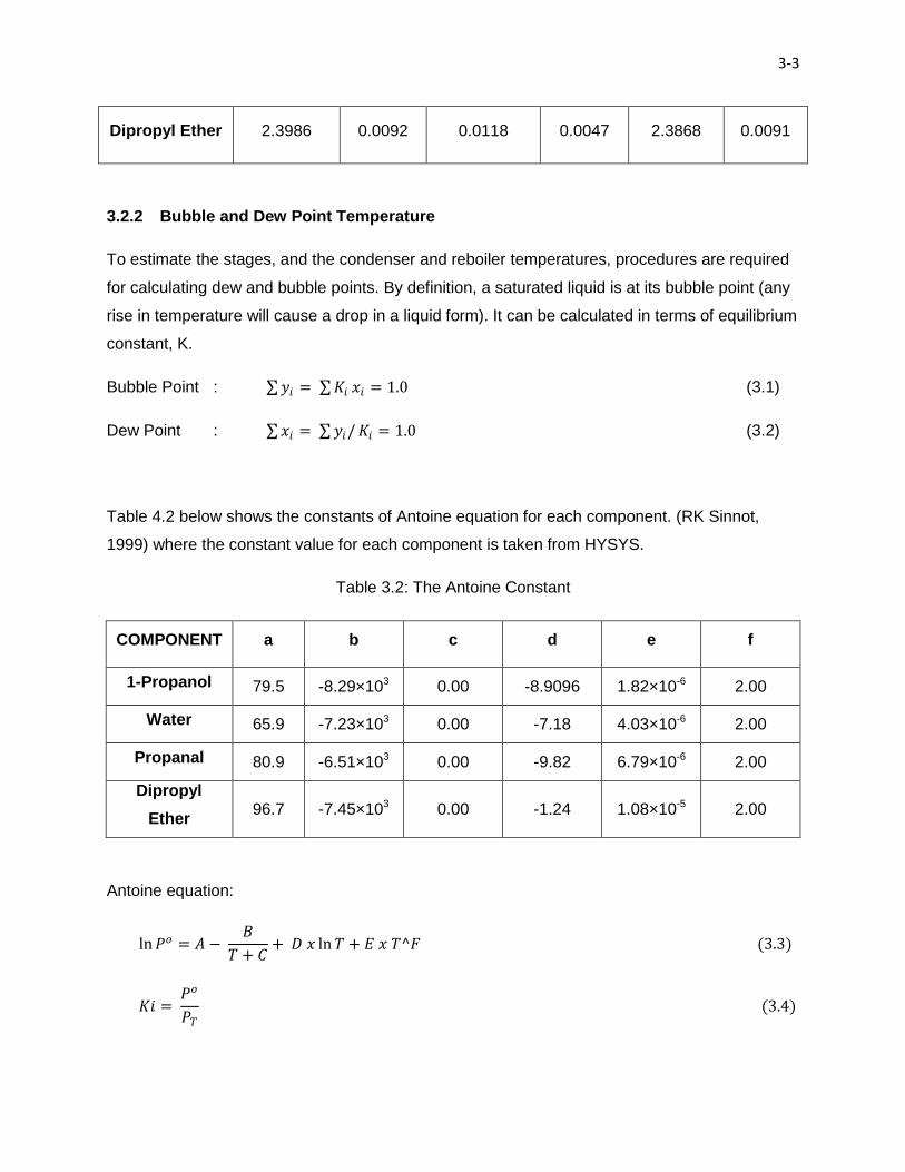
Dipropyl Ether 2.3986 0.0092 0.0118 0.0047 2.3868 0.0091
3.2.2 Bubble and Dew Point Temperature
To estimate the stages, and the condenser and reboiler temperatures, procedures are required
for calculating dew and bubble points. By definition, a saturated liquid is at its bubble point (any
rise in temperature will cause a drop in a liquid form). It can be calculated in terms of equilibrium
constant, K.
Bubble Point : 𝑦𝑖 = 𝐾𝑖 𝑥𝑖 = 1.0 (3.1)
Dew Point : 𝑥𝑖 = 𝑦𝑖/ 𝐾𝑖 = 1.0 (3.2)
Table 4.2 below shows the constants of Antoine equation for each component. (RK Sinnot,
1999) where the constant value for each component is taken from HYSYS.
Table 3.2: The Antoine Constant
COMPONENT a b c d e f
1-Propanol 79.5 -8.29×10³ 0.00 -8.9096 1.82×10⁻⁶ 2.00
Water 65.9 -7.23×10³ 0.00 -7.18 4.03×10⁻⁶ 2.00
Propanal 80.9 -6.51×10³ 0.00 -9.82 6.79×10⁻⁶ 2.00
Dipropyl
Ether 96.7 -7.45×10³ 0.00 -1.24 1.08×10⁻⁵ 2.00
Antoine equation:
ln 𝑃𝑜 = 𝐴 − 𝐵
𝑇 + 𝐶+ 𝐷 𝑥 ln 𝑇 + 𝐸 𝑥 𝑇^𝐹 (3.3)
𝐾𝑖 = 𝑃𝑜
𝑃𝑇 (3.4)

3-4
Estimation of feed temperature, 𝑥𝑖 = 𝑦𝑖/ 𝐾𝑖 = 1.0
By using the goal seek method in the excel program, with constant operating pressure at feed is
1.6 bar, the calculated temperature is 363K. The data shown in Table 3.3:
Table 3.3: Calculation of Bubble Point at Feed Stream
COMPONENT ln Pi Pi (kPa) Xi O.P
(kPa) Ki Yi=KiXi
1-Propanol 5.19 179.42 0.9768 182 0.99 0.962939
Water 5.07 159.48 0.0085 182 0.88 0.007448
Propanal 6.54 692.20 0.0055 182 3.80 0.020918
Dipropyl Ether 5.23 186.62 0.0092 182 1.03 0.009434
TOTAL 1.00000
Hence, the bubble point temperature is 386.36 K
By using the goal seek method in the excel program, with constant operating pressure at top is
0.5 bar, the calculated temperature is 60K. The data shown in Table 3.4:
Dew Point Temperature (top column) 𝑥𝑖 = 𝑦𝑖/ 𝐾𝑖 = 1.0
Table 3.4: Calculation of Dew Point at Top Column
COMPONENT ln Pi Pi (kPa) Yi O.P
(kPa) Ki Xi=Yi/Ki
1-Propanol 3.59 36.41 0.4853 50 0.73 0.67
Water 3.54 34.59 0.1817 50 0.69 0.26
Propanal 5.44 231.56 0.3068 50 4.63 0.07
Dipropyl Ether 4.01 55.25 0.0047 50 1.10 0.004
TOTAL 1

3-5
Hence, the dew point temperature is 345.56 K
By using the goal seek method in the excel program, with constant operating pressure at bottom
is 1.6 bar, the calculated temperature is 376K. The data shown in Table 3.5:
Bubble Point Temperature (bottom column) 𝑦𝑖 = 𝐾𝑖 𝑥𝑖 = 1.0
Table 3.5: Calculation of Bubble Point at Bottom Column
COMPONENT ln Pi Pi (kPa) Xi O.P
(kPa) Ki Yi=KiXi
1-Propanol 4.69 108.95 0.9815 110 0.99 0.97
Water 4.59 98.45 0.0068 110 0.89 0.01
Propanal 6.20 490.93 0.0026 110 4.46 0.01
Dipropyl Ether 4.85 127.18 0.0091 110 1.16 0.01
TOTAL 1
Hence, the bubble point temperature is 372.33 K
3.2.3 Determination of Relative Volatility
The equilibrium vaporization constant K is defined for a compound by
𝐾𝑖 = 𝑌𝑖
𝑋𝑖 (3.5)
Where, Yi = mole fraction of component i in vapour phase
Xi = mole fraction of component i in liquid phase
The relative volatility, α which is needed in the calculation is defined as
𝛼𝑖𝑗 = 𝐾𝑖
𝐾𝑗 (3.6)

3-6
Where i and j represent the components to be separated
From Ideal system, Raoult’s law,
Pi = PiXi (3.7)
The relative volatility of two components can be expressed as the ratio of their K value,
𝛼𝑖𝑗 = 𝐾𝐿𝐾
𝐾𝐻𝐾 (3.8)
Where, KLK = Light key components
KHK = Heavy key components
3.2.3.1 Top Column
Table 3.6
COMPONENT K 𝜶 = 𝑲
𝑲𝑯𝑲
1-Propanol 0.7300 0.6636
Water 0.6900 0.6273
Propanal 4.6300 4.2091
DPE 1.1000 1.0000
3.2.3.2 Bottom Column
Table 3.7
COMPONENT K 𝜶 = 𝑲
𝑲𝑯𝑲
1-Propanol 0.9900 0.8534
Water 0.8900 0.7672
Propanal 4.4600 3.8448

3-7
DPE 1.1600 1.0000
Average relative volatility of the light key to heavy key;
αLK = Top α (Bottom α)
= 0.6636 (0.8534)
= 0.753
3.2.4 Minimum Number of Stages Using Fenske’s Equation
The Fenske’s Equation (1932) can be used to estimate the minimum stages required at total
reflux. The derivation of the equation for binary system and applies equally to multi-component
system. The minimum number of stages will be obtained from this equation:
Nmin = Log[(
XLK
XHK)]d[(
XHK
XLK)]b
Log αLK (3.9)
= Log[(
0.731.1 )]d[(
0.00910.9815
)]b
Log 0.753
= 17.94
= 20 stages
3.2.5 Minimum Reflux Ratio
Colburn (1941) and Underwood (1948) have derived equations for estimating the minimum
reflux ratio for multicomponent distillations. The equation can be stated in the form:
𝛼𝑖𝑥𝑖,𝑑
𝛼𝑖 − 𝜃= 𝑅𝑚 + 1 (3.10)

3-8
Where,
αi = the relative volatility of component i with respect to some reference
component, usually the heavy key
Rm = the minimum reflux ratio
Xi,d = concentration of component i in the tops at minimum reflux
and θ is the root of the equation:
𝛼𝑖𝑥𝑖 ,𝑓
𝛼𝑖 − 𝜃= 1 − 𝑞 (3.11)
Where,
Xi,f = the concentration of component i in the feed, and q depends on the
condition of the feed
The value of θ must lie between the values of relative volatility of the light and heavy keys and is
found by trial and error.
As the feed at its boiling point q = 1
𝛼𝑖𝑥𝑖 ,𝑓
𝛼𝑖 − 𝜃= 0
Table 3.8
Component Xi,f αi αiXi,f θ estimate (αiXi,f)/(αi - θ)
1-Propanol 0.9768 0.7600 0.7424 3.9 -0.2364
Water 0.0085 0.7000 0.0060 3.9 -0.0019
Propanal 0.0055 4.0300 0.0222 3.9 0.1705
DPE 0.0092 1.0000 0.0092 3.9 -0.0032
3.9 -0.07
Therefore, θ = 3.9

3-9
Table 3.9
Component Xi,d αi αiXi,d θ estimate (αiXi,d)/(αi - θ)
1-Propanol 0.4853 0.76 0.3688 3.9 -0.1175
Water 0.1817 0.7 0.1272 3.9 -0.0397
Propanal 0.3068 4.03 1.2364 3.9 9.5108
DPE 0.0047 1 0.0047 3.9 -0.0016
3.9 9.35
Taking equation 3.10,
Rm + 1 = 9.35
Rm = 8.35
𝑅𝑚
𝑅𝑚 + 1= 0.8931
Specimen calculation, for R = 2.0
𝑅
(𝑅 + 1)=
2
3= 0.66
Using Erbar – Maddox correlation (Erbar and Maddox, 1961) from figure 11.11 (Coulson and
Richardson, Volume 6, page 524),
𝑁𝑚
𝑁= 0.74
N = 18
0.74
= 24.3
For other reflux ratios
R 2 3 4 5
N 24.3 21.43 20.69 20.22

3-10
The optimum reflux ratio will be near to 4. Therefore, the optimum reflux ratio will be taken as 4
while the actual stage is 21.
3.2.6 Feed Point Location
Feed point location can be found using Kirkbride (1944) equation:
𝐿𝑜𝑔 𝑁𝑟
𝑁𝑠= 0.2606 log
𝐵
𝐷
𝑥𝑓 ,𝐻𝐾
𝑥𝑓 ,𝐿𝐾
x𝑏 ,𝐿𝐾
x𝑑 ,𝐻𝐾
2
(3.10)
Where,
Nr = no. of stages above the feed, including any partial condenser
Ns = no. of stages below the feed, including the reboiler
B = molar flow bottom product
D = molar flow top product
Xf,HK = concentration of the heavy key in the feed
Xf,LK = concentration of the light key in the feed
Xd,HK = concentration of the heavy key in the top product
Xb,HK = concentration of the heavy key in the bottom product
𝐿𝑜𝑔 𝑁𝑟
𝑁𝑠= 0.2606 log
2.531
261.5
0.0092
0.9768
0.395
0.00382
2
𝑁𝑟
𝑁𝑠 = 0.993
Actual number of plates is 24
Nr + Ns = 24
0.993Ns + Ns = 24
1.993Ns = 9

3-11
Nr = 15
So, feed inlet is at stage 9 from bottom.
3.2.7 Efficiency of Distillation Column
Overall column efficiency is given as:
𝐸˳ = 51 − 32.5 log (µ𝑎𝜍𝑎) (3.11)
Where,
µ𝑎 = the molar average liquid viscosity, mNs/m2
𝜍𝑎 = average relative volatility of the light key
To find the viscosity of the flow:
𝐿𝑂𝐺 µ𝑎 = 𝑉𝑖𝑠𝐴 𝑥 1
𝑇 −
1
𝑉𝑖𝑠𝐵 (3.12)
Table 3.8 Viscosity of the mixture
Component Mole fraction
feed, x
Viscosity Coefficient
Log µ𝒂 Viscosity (mNs/m2)
µ𝒂 × 𝒙
A B
1-Propanol 0.9768 951.04 327.83 -0.32859 0.46926 0.4584
Water 0.0085 658.25 283.16 -0.54418 0.28564 0.0024
Propanal 0.0055 343.44 219.33 -0.63690 0.23073 0.0013
DPE 0.0092 410.58 219.67 -0.75852 0.17438 0.0016
TOTAL 1.16 0.4637
Where,
𝐸 ˳ = 51 − 32.5 log (µ𝑎𝜍𝑎)

3-12
= 51 – 32.5 log (0.463674405 x 0.787)
= 55.44 %
Plate and overall column efficiencies will normally be between 30% to 70%. (Coulson and
Richardson’s, volume 6, page 547)
3.2.8 Physical Properties
3.2.8.1 Relative Molar Mass (RMM)
RMM = ∑ (component mole fraction x molecular weight) (3.13)
Table 3.9 Liquid Density
Component Molecular
Weight
Mole Fraction Liquid Density
(kg/m3) Feed Distillate Bottom
1-Propanol 60.1 0.9768 0.4853 0.9815 803.4
Water 18.015 0.0085 0.1817 0.0068 1000
Propanal 58.08 0.0055 0.3068 0.0026 810
DPE 102.18 0.0092 0.0047 0.0091 725
Feed, F = 0.9768 (60.1) + 0.0085 (18.015) + 0.0055 (58.08) + 0.0092 (102.18)
= 60.118 kg/kmol
Distillate, D = 0.4853 (60.1) + 0.1817 (18.015) + 0.3068 (58.08) + 0.0047 (102.18)
= 50.739 kg/kmol
Bottom, B = 0.9815 (60.1) + 0.0068 (18.015) + 0.0026 (58.08) + 0.0091 (102.18)
= 60.191 kg/kmol

3-13
3.2.8.2 Density
Top Product :
ρL = 𝑥𝐵,𝑖 𝜌𝑖 (3.14)
ρL = 0.4835(803.4) + 0.1817(100) + 0.3068(810) + 0.0047(725)
= 823.51 kg/m3
ρv = 𝑅𝑀𝑀𝐵
𝑉𝑆𝑇𝑃 𝑥
𝑇𝑆𝑇𝑃
𝑇𝑂𝑃 𝑥
𝑃𝑂𝑃
𝑃𝑆𝑇𝑃 (3.15)
ρv = 29.167 𝑘𝑔/𝑘𝑚𝑜𝑙𝑒
22.4𝑚3/𝑘𝑚𝑜𝑙𝑒 𝑥
273𝐾
357.21𝐾 𝑥
1𝑏𝑎𝑟
1𝑏𝑎𝑟
= 1.731 kg/m3
Bottom Product:
ρL = 𝑥𝐷,𝑖 𝜌𝑖 (4.16)
ρL = 0.9815(803.4) + 0.0068(100) +0.0026(810) + 0.0091(725)
= 804.04 kg/m3
ρv = 𝑅𝑀𝑀𝐷
𝑉𝑆𝑇𝑃 𝑥
𝑇𝑆𝑇𝑃
𝑇𝑂𝑃 𝑥
𝑃𝑂𝑃
𝑃𝑆𝑇𝑃 (4.17)
ρv = 58.988𝑘𝑔/𝑘𝑚𝑜𝑙𝑒
22.4𝑚3/𝑘𝑚𝑜𝑙𝑒 𝑥
273𝐾
382.2𝐾 𝑥
1.6𝑏𝑎𝑟
1𝑏𝑎𝑟
= 3.071 kg/m3
3.2.8.3 Surface Tension, σ
Using Sugden (1924), equation 8.23 (Coulson and Richardson’s, volume 6, page 335)
𝜍 = 𝑃𝑐(𝜌𝑙 − 𝜌𝑣
𝑀
4
𝑥 10−12 (3.18)
3-14
Where,
σ = surface tension, MJ/m2 or (dyne/cm)
Pch = Sugden’s parachor
ρv = Vapor density, kg/m3
ρL = Liquid density, kg/m3
M = relative molecular weight
For mixture, σm = σ1x1 + σ2x2 + ….. (3.19)
Where,
σm = surface tension mixture
σ1 , σ2 = surface tension for mixture
x1 , x2 = component mole fraction
Table 3.10 Pch Distribution
Component Pch
Distribution
Mole Fraction
Distillate Bottom
1-Propanol 148.3 0.4853 0.9815
Water 31.3 0.1817 0.0068
Propanal 165.4 0.3068 0.0026
DPE 299.5 0.0047 0.0091
Pch at top = 𝑥𝐷,𝑖 𝑃𝑐𝑖
= 0.4853 (148.3) + 0.1817 (31.3) + 0.3068 (165.4) + 0.0047 (299.5)

3-15
= 177.28097
Pch at bottom = 𝑥𝐵,𝑖 𝑃𝑐𝑖
= 0.9815 (148.3) + 0.0068 (31.3) + 0.0026 (165.4) + 00.0091 (299.5)
= 148.30792
Calculation of surface tension:
Top Column, 𝜍 = 65.01 969.64−4.928
21.98
4
𝑥 10−12
= 67.965683 N/m
Bottom Column, 𝜍 = 59.04 1019.01− 0.325
20.04
4
𝑥 10−12
= 15.27159545 N/m
Above feed point:
Vapor flow rate: Vn = D(R + 1) (3.20)
Where,
D = Distillate molar flowrate
R = Reflux ratio
Hence,
Vn = 261.5 (2.531 + 1)
= 923.36 kmole/hr
Liquid down flow: Ln = Vn – D (3.21)
= 923.36 – 261.5

3-16
= 661.86 kmole/hr
Below the feed point:
Liquid flow rate: Lm = Ln + F (3.22)
Where,
F = Feed molar flowrate
Hence,
Lm = 661.86 + 264.1
= 925.96kmole/hr
Vapour flow rate: Vm = Lm – W (3.23)
Where,
W = Bottom molar flowrate
Hence,
Vm = 925.96 – 261.5
= 664.46kmole/hr
The equation for the operating lines below the feed plate:
𝑌𝑚 = 𝐿𝑚
𝑉𝑚 𝑋𝑚 + 1 −
𝑊
𝑉𝑚 𝑋𝑤 (3.24)
𝑌𝑚 = 925.96
664.46 𝑋𝑚 + 1 −
261.5
664.46 (𝑋𝑤)
= 2.058(Xm + 1) – 261.5
664.46 (𝑋𝑤)
The equation for the operating lines above the feed plate:
𝑌𝑛 = 𝐿𝑛
𝑉𝑛 𝑋𝑛 + 1 −
𝐷
𝑉𝑛 𝑋𝑑 (3.25)

3-17
𝑌𝑛 = 661.86
923.36 𝑋𝑛 + 1 −
261.5
923.36 𝑋𝑑
= 0.72 (Xn + 1) – 2.01 x 10⁻³
𝐹𝐿𝑉 𝑇𝑜𝑝 = 𝐿𝑛
𝑉𝑛
𝜌𝑉
𝜌𝐿 (3.26)
= 0.72 1.731
823.51
= 0.033
where 0.72 is the slope of the top operating line.
𝐹𝐿𝑉 𝐵𝑜𝑡𝑡𝑜𝑚 = 𝐿𝑚
𝑉𝑚
𝜌𝑉
𝜌𝐿 (3.27)
= 1.39 3.071
804.04
= 0.09
where 1.39 is the slope of the bottom operating line.
3.2.9 Determination of Plate Spacing
The overall height of the column will depend on the plate spacing. Plate spacing from 0.15m to
1.0m are normally used. The spacing chosen will depend on the column diameter and the
operating condition. Close spacing is used with small - diameter columns, and where head room
is restricted, as it will be when a column is installed in a building. In this distillation column, the
plate spacing is 0.5m as it is normally taken as the initial estimate recommended by Coulson
and Richardson’s, Chemical Engineering, Volume 6.

3-18
The principal factor that determines the column diameter is the vapor flowrate. The
vapor velocity must be below that which would cause excessive liquid entrainment or high-
pressure drop. The equation below which is based on the Souder and Brown equation,
Lowenstein (1961), Coulson & Richarson’s Chemical Engineering, Volume 6, page 556, can be
used to estimate the maximum allowable superficial velocity, and hence the column area and
diameter of the distillation column.
𝑈𝑣 = −0.171𝑙𝑡2 + 0.271𝑙𝑡 − 0.047
𝜌𝐿 − 𝜌𝑣
𝜌𝑣
0.5
(3.28)
= −0.171(0.5)2 + 0.271(0.5) − 0.047 969.64 − 4.928
4.928
0.5
= 2.8173 m/s
Where,
Uv = maximum allowable vapor velocity based on the gross (total) column cross
Sectional area, m/s
lt = plate spacing, m (range: 0.5 – 1.5)
3.2.9.1 Diameter of the column
𝐷𝑐 = 4𝑉𝑤
𝜋𝜌𝑣 𝑈𝑣 (3.29)
Where Vw is the maximum vapor rate, kg/s
𝑉𝑤 = 15870 𝑘𝑔
𝑟 𝑥
1 𝑟
3600 𝑠
= 4.41 kg/s
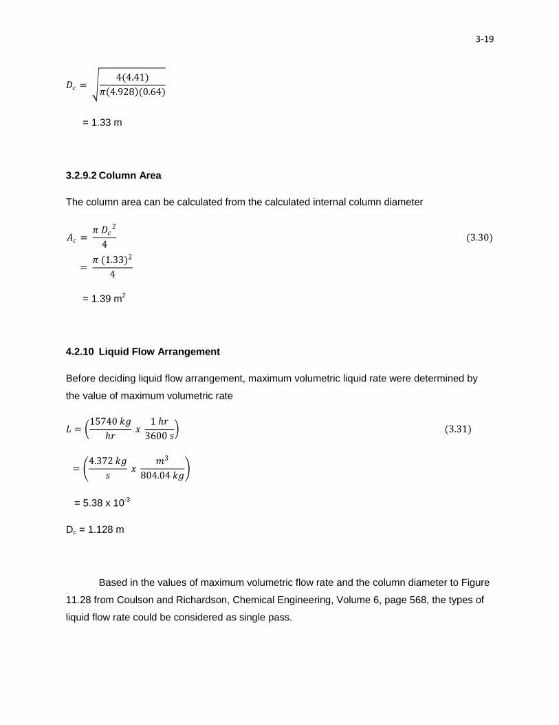
3-19
𝐷𝑐 = 4(4.41)
𝜋 4.928 (0.64)
= 1.33 m
3.2.9.2 Column Area
The column area can be calculated from the calculated internal column diameter
𝐴𝑐 = 𝜋 𝐷𝑐
2
4 (3.30)
= 𝜋 (1.33)2
4
= 1.39 m2
4.2.10 Liquid Flow Arrangement
Before deciding liquid flow arrangement, maximum volumetric liquid rate were determined by
the value of maximum volumetric rate
𝐿 = 15740 𝑘𝑔
𝑟 𝑥
1 𝑟
3600 𝑠 (3.31)
= 4.372 𝑘𝑔
𝑠 𝑥
𝑚3
804.04 𝑘𝑔
= 5.38 x 10⁻³
Dc = 1.128 m
Based in the values of maximum volumetric flow rate and the column diameter to Figure
11.28 from Coulson and Richardson, Chemical Engineering, Volume 6, page 568, the types of
liquid flow rate could be considered as single pass.

3-20
Perforated plate, which is famously known as sieve tray is the simplest type of cross-flow
plate. Cross flow trays are the most common used and least expensive. Sieve tray is chosen
because it is consider cheaper and simpler contacting devices. The perforated trays enable
designs with confident prediction of performance. According, most new designs today specify
some type of perforated tray (sieve tray) instead of the traditional bubble-cap tray. Sieve tray
also gives the lowest pressure drop.
3.2.11 Plate Design
Column diameter, Dc = 1.33 m
Column area, Ac = 1.39 m2
As a first trial, take the downcomer area as 12% of the total
Downcomer area, Ad = 0.12 Ac (3.32)
= 0.12 x 1.39 m2 = 0.1668 m2
Net area, An = Ac - Ad (3.33)
= 1.39 m2 - 0.1668 m2
= 1.2232 m2
Active area, Aa = Ac – 2Ad (3.34)
= 1.39 m2 – 2(0.1668 m2)
= 1.0564 m2
Assume that the hole-active area is 10%
Hole area, Ah = 0.10 Aa (3.35)
= 0.10 x 1.0564 m2
= 0.10564m2

3-21
3.2.11.1 Weir Length
With segmental downcomers the length of the weir fixes the area of the downcomer. The chord
length will normally be between 0.6 to 0.85 of the column diameter. A good initial value to use is
0.77, equivalent to a downcomer area of 15%.
Referring to Figure 11.31 from Coulson and Richardson’s, Chemical Engineering, Volume 6,
page 572, with (Ad/Ac) x 100 is 12 percents, thus, Iw/Dc is 0.76
Weir length, Iw = 0.76Dc
= 0.76 x 1.33 m
= 1.011 m
3.2.11.2 Weir Height
For column operating above atmospheric pressure, the weir-heights will normally be between 40
mm to 90 mm (1.5 to 3.5 in); 40 to 50 mm is recommended.
Take Weir height, hw = 50 mm
Hole diameter, dh = 5 mm (preferred size)
Plate thickness, t = 3 mm (stainless steel)
For hole diameter = 5 mm, area of one hole,
𝐴𝑙 = 𝜋(𝑑)2
4 (3.36)
= 𝜋(0.005)2
4
= 1.9635 x 10⁻⁵ m2

3-22
Number of holes per plate,
𝑁 = 𝑎𝑟𝑒𝑎
1 𝑜𝑙𝑒 𝑎𝑟𝑒𝑎 (3.37)
= 0.10564
1.9635 𝑥 10−5
= 5380.19 holes
≈ 5380 holes
3.2.11.3 Weir Liquid Crest
Check weeping to ensure enough vapour to prevent liquid flow through hole.
𝑀𝑎𝑥𝑖𝑚𝑢𝑚 𝑙𝑖𝑞𝑢𝑖𝑑 𝑟𝑎𝑡𝑒 = 15740𝑘𝑔
𝑟 𝑥
1 𝑟
3600 𝑠
= 4.372 kg/s
Minimum liquid rate, at 70% turndown
= 0.7 x 4.372 kg/s
= 3.06 kg/s
The weir liquid can be determine by using the equation below
𝑜𝑤 = 750 𝐿𝑤
𝜌𝐿𝐼𝑤
23
(3.38)
Where,
Iw = weir length, m
Lw = liquid flow rate, kg/s
ρL = liquid density, kg/m3
3-23
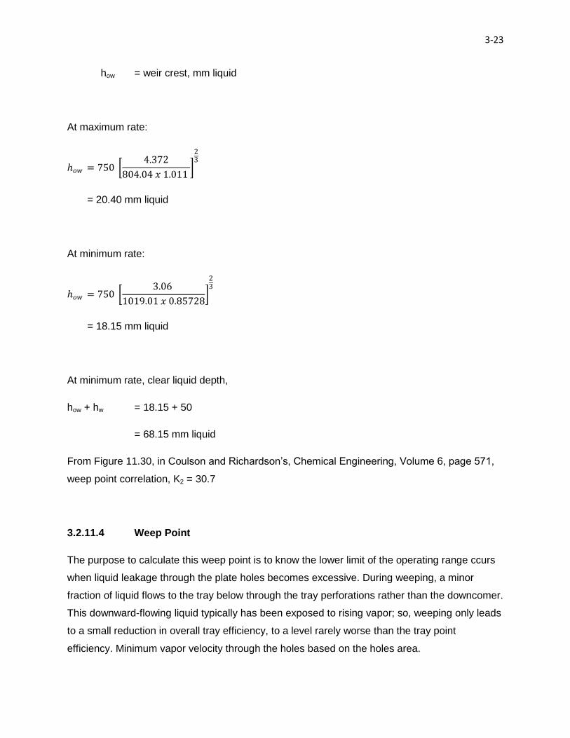
how = weir crest, mm liquid
At maximum rate:
𝑜𝑤 = 750 4.372
804.04 𝑥 1.011
23
= 20.40 mm liquid
At minimum rate:
𝑜𝑤 = 750 3.06
1019.01 𝑥 0.85728
23
= 18.15 mm liquid
At minimum rate, clear liquid depth,
how + hw = 18.15 + 50
= 68.15 mm liquid
From Figure 11.30, in Coulson and Richardson’s, Chemical Engineering, Volume 6, page 571,
weep point correlation, K2 = 30.7
3.2.11.4 Weep Point
The purpose to calculate this weep point is to know the lower limit of the operating range ccurs
when liquid leakage through the plate holes becomes excessive. During weeping, a minor
fraction of liquid flows to the tray below through the tray perforations rather than the downcomer.
This downward-flowing liquid typically has been exposed to rising vapor; so, weeping only leads
to a small reduction in overall tray efficiency, to a level rarely worse than the tray point
efficiency. Minimum vapor velocity through the holes based on the holes area.

3-24
𝑈(min) = 𝐾2 − 0.9(25.4 − 𝑑)
𝜌𝑣
12
(3.39)
Where,
Uh = minimum vapor velocity, m/s
dh = hole diameter, mm
K2 = constant
= 30.7 − 0.9(25.4 − 5)
(3.071)12
= 8.036 m/s
𝐴𝑐𝑡𝑢𝑎𝑙 𝑚𝑖𝑛𝑖𝑚𝑢𝑚 𝑣𝑎𝑝𝑜𝑟 𝑣𝑒𝑙𝑜𝑐𝑖𝑡𝑦 = 𝑀𝑖𝑛𝑖𝑚𝑢𝑚 𝑣𝑎𝑝𝑜𝑟 𝑟𝑎𝑡𝑒
𝐴 (3.40)
=
4.41 𝑘𝑔𝑠
𝑥 0.7 𝑥 𝑚3
3.071𝑘𝑔
0.10564
= 9.51 m/s
So, minimum operating rate will be above weep point.
3.2.12 Plate Pressure Drop
Maximum vapor velocity through holes:
Û = 𝑚𝑎𝑥𝑖𝑚𝑢𝑚 𝑣𝑎𝑝𝑜𝑟 𝑓𝑙𝑜𝑤𝑟𝑎𝑡𝑒
𝐴 (3.41)

3-25
=
4.41 𝑘𝑔𝑠
𝑥 𝑚3
3.071 𝑘𝑔
0.10564
= 13.59 m/s
From Figure 11.34 in Coulson and Richardson’s, Chemical Engineering, Volume 6, page 576,
for discharge coefficient for sieve plate,
𝐴𝑡, 𝑝𝑙𝑎𝑡𝑒 𝑡𝑖𝑐𝑘𝑛𝑒𝑠𝑠
𝑜𝑙𝑒 𝑑𝑖𝑎𝑚𝑒𝑡𝑒𝑟=
3 𝑚𝑚
5 𝑚𝑚= 0.6
𝑎𝑛𝑑 𝐴
𝐴𝑎= 0.1
we get Co = 0.74
𝐷𝑟𝑦 𝑝𝑙𝑎𝑡𝑒, 𝑑 = 51 𝑈
𝐶𝑜
2
𝜌𝑣
𝜌𝐿 (3.42)
= 51 13.59
0.74
2
3.071
804.04
= 65.697 mm liquid
𝑅𝑒𝑠𝑖𝑑𝑢𝑎𝑙 𝑒𝑎𝑑, 𝑟 = 12.5 𝑥 103
𝜌𝐿 (3.43)
= 12.5 𝑥 103
804.04
= 15.55 mm liquid
Pressure drop per plate, ht = hd + (hw + how) + hr (3.44)
= 65.697 + (50 + 18.15) + 15.55
= 149.397 mm liquid

3-26
3.2.13 Downcomer Liquid Back-Up
The downcomer area and plate spacing must be such that the level of the liquid and froth in the
downcomer is well below the top of the outlet weir on the plate above. If the level rises above
the outlet weir the column will flood.
Take hap = hw – 10 mm
= 50 – 10
= 40 mm
Where, hap = height of the bottom edge of the apron above the plate
𝑑𝑐 = 166 𝐿𝑤𝑑
𝜌𝐿𝐴𝑚
2
(3.45)
Where,
Lwd = liquid flowrate in downcomer, kg/s
Am = either the downcomer area, Ad or the clearance area under the downcomer, Aap
whichever is smaller, m2
Area under apron,
Aap = hap x Iw (3.46)
= 0.04 m x 1.011
= 0.04044 m2
Where, Aap = the clearance area under downcomer
As this less than Ad = 0.1668 m2, equation 11.92 (Coulson and Richardson’s, Volume 6, page
577) used Aap = 0.04044 m2

3-27
𝑑𝑐 = 166 4.372
804.04 𝑥 0.04044
2
= 3.00 mm
3.2.14 Backup on Downcomer
hb = (hw + how) + ht + hdc (3.47)
= (50 + 18.15) +149.397 +3.00
= 220.547 mm
hb < ½(plate spacing + weir height)
0.2205 m < ½(0.5 + 0.05) m
0.2205 m <0.5 m
So, tray spacing = 0.5 m is acceptable (to avoid flooding).
3.2.15 Residence Time
Sufficient residence time must be allowed in the downcomer for the entrained vapor to
disengage from the liquid stream, to prevent heavily “aerated” liquid being carried under the
downcomer. A time at least 3 seconds is recommended.
𝑡𝑟 = 𝐴𝑑𝑏𝑐𝜌𝐿
𝐿𝑤𝑑 (3.48)
Where,
tr = residence time, s
Lwd = liquid flowrate in downcomer, kg/s
hbc = clear liquid back up in the downcomer, m

3-28
𝑡𝑟 = 0.1668 𝑥 0.2205𝑥 804.04
4.372
= 6.764 s
tr is greater than 3.0 which is recommended so tr is satisfactory.
3.2.16 Perforated Area
From Figure 11.32, Coulson and Richardson’s, Chemical Engineering, Volume 6, page 527, for
the relaxation between angle subtended by chord, chord height and chord length:
Iw/Dc = 1.011/1.33
= 0.76
θ = 98°
Ih/Dc = 0.18
Angle subtended at plate edge by unperforated strips
= 180° - 98°
= 82°
Mean length, unperforated edge strips
= (Dc – weir height) x π x θ/180°
= (1.33 – 0.05) x π x 82°/180°
= 1.832 m
Areas of unperforated edge strips, As
= mean length unperforated edge x weir height
= 1.832 x 0.05
= 0.0916 m2

3-29
Mean length of calming zone = Weir length + Width of unperforated strip
= 1.011 + 0.05
= 1.061 m
Area of calming zone = 2 x (weir height x mean length calming zone)
= 2 x 0.05 x 1.061
= 0.1061 m2
Total area available for perforation, Ap :
= Active area – (area of unperforated edge + area of calming)
= 1.0564 – (0.0916 + 0.1061)
= 0.8587 m2
Ah/Ap = 1.0564/0.8587
= 0.123
From Figure 11.33, Coulson and Richardson’s, Chemical Engineering, Volume 6, page 528, the
relation between hole area and pitch,
Ip/dh = 2.7; satisfactory, which is within 2.5 to 4.0
3.2.17 Column Size
The column height will be calculated based on the given below. The equation determines the
height of the column without taking the skirt or any support into consideration. Its determination
is based on the condition in the column.
Column height = (No. of stages – 1) x (Tray spacing ) + (Tray spacing x 2) + (No. of stages – 1)

3-30
x (Plate thickness)
= (24 – 1)(0.5) + (24 – 1)(0.003)
= 11.57 m
By adding 10% safety factor so the column height are 12.7 m ≈ 13 m
3.2.18 Plate Design Specification
Table 3.10 Summary of Plate Design
Item Value
Column Diameter, Dc 1.33 m
No. of Plates 24 plates
Plate Spacing 0.5 m
No. of Stage Feed from bottom, F1 9
No. of Stage Solvent from bottom, F2 24
Plate Thickness 0.003 m
Total Column Height, Ht 13 m
Plate Material Stainless Steel
Downcomer Area, Ad 0.1668 m2
Column Area, Ac 1.39 m2
Net Area, An 1.2232 m2
Active Area, Aa 0.10564 m2
Hole Area, Ah 0.010564 m2
No. of Holes 5380 units
Weir Length, Iw 1.011 m
Weir Height (standard) 0.05 m

3-31
3.3 Mechanical Design
3.3.1 Introduction
Several factors need to be considered in the mechanical design of distillation column such as
1. Design pressure
2. Design temperature
3. Material of construction
4. Design stress
5. Wall thickness
6. Welded joint efficiency
7. Analysis of stresses
a. Dead weight load
b. Wind load
c. Pressure stress
d. Bending stress
8. Vessel support
9. Insulation
3.3.2 Column Design Specification
Operating pressure = (1.82 – 1) bar
= 0.82 bar
Take as 10% above operating pressure
Design pressure = 0.82 x 1.1
=0.902 bar
= 0.0902 N/mm2
Design temperature = 113.36°C
Take as 10% above operating temperature
Operating temperature = 113.36 x 1.1
= 124.694°C

3-32
3.3.3 Material of Constructions
Selection of suitable material must be taking onto account the suitability of material for
fabrication (particularly welding) as well as the compatibility of the material with the process
environment. In this case, the material used in the construction of the distillation column is
carbon steel as the material as it is the most used material in industry. For this material, the
design stress at 150°C is obtained from Table 13.2 for the typical design stresses for plate.
Design stress, f = 115 N/mm2
Tensile strength = 360 N/mm2
Join factor = 1
Diameter vessel, D = 1330 mm
Operating pressure = 0.0902 N/mm2
Insulation, mineral wool = 75 mm thick
3.3.4 Vessel Thickness
The minimum thickness of column required and other designs are calculated based on equation
below:
ℯ = 𝑃𝑖𝐷𝑖
2𝐽𝑓 − 𝑃𝑖 3.49
Where,
e = minimum thickness of the plate required
Pi = internal pressure, N/mm2
Di = internal diameter, m
f = design stress, N/mm2
J = joint factor
Therefore, minimum thickness required,
ℯ = 0.0902 𝑥 1330
2 1 (115) − 0.0902
= 0.522 mm
≈ 0.6 mm

3-33
A much thicker wall is needed at the column base to withstand the wind and dead weight loads.
As a first trial, divide the column into five sections, with the thickness increasing by 2 mm per
section. Try 1, 3, 5, 7 and 9 mm. The average wall thickness is 5 mm. Take the first trial as 5
mm.
3.3.5 Heads and Closure
Hemispherical, ellipsoidal and torispherical heads are collectively referred to as domed heads.
They are formed by pressing or spinning, large diameters are fabricated from formed sections.
Torispherical are often referred to as dished ends. After comparing the thickness of all heads,
torispherical head had been chosen because of operating pressure for this below 10 bars and
suitable for liquid vapor phase process in inconsistent high pressure. The thickness of
torispherical head can be calculated below:
ℯ = 𝑃𝑖𝑅𝑐𝐶𝑠
2𝐽𝑓 + 𝑃𝑖(𝐶𝑠 − 0.2) 3.50
Where,
Rc = Crown radius = Dc
Rk = Knuckle radius = 0.06 Rc
= 0.06 x 1330
= 79.8 mm
Cs = Stress concentration
= 1
4 3 +
𝑅𝑐
𝑅𝑘
= 1
4 3 +
1330
79.8
= 1.77
ℯ = 0.0902 × 1330 × 1.77
2 1 (115) + 0.09(1.77 − 0.2) 3.51
= 0.923 mm
Round up to 2 mm

3-34
For welding purposes the thickness of head were taken as same thickness of the vessel, = 2
mm. It’s matching to joint factor were taken as 1.
3.3.6 Weight Loads
The major sources of the dead weight loads are:
1. The vessel shell
2. The vessel fittings: manhole, nozzles
3. Internal fitting: plates, heating cooling coils
4. External fittings: ladders, platforms, piping
5. Auxiliary equipment which is not self supported, condensers, agitators
6. Insulation
7. The weight of liquid to fill the vessel.
3.3.6.1 Dead Weight of Vessel
Dead weight of vessel can be calculated by using equation below:
Wv = 240 x Cv x Dm x (Hv + 0.8 Dm)t x 10-3 kN (3.52)
Where,
Wv = total weight of shell, excluding internal fitting such as plates
Cv = a factor to account for the weight of nozzles, man ways and internal supports.
(In this distillation column, take Cv as 1.15)
Dm = mean diameter of vessel
= (Dc + t) m
= (1.33 + 0.007)
= 1.337 m
Hv = height or length between tangent lines, m
t = wall thickness, m
Wv = 240 x 1.15 x 1.337(13.0 + 0.8(1.337)) x 0.007
= 36.34 kN

3-35
3.3.6.2 Weight of Plate, Wp
From Nelson Guide, page 833 Chemical Engineering Volume 6; take contacting plates, 1.2
kN/m2 (for typical liquid loading). The total of weight of plate determine by multiply the value with
number of plate design.
𝑃𝑙𝑎𝑡𝑒 𝑎𝑟𝑒𝑎 = 𝜋𝐷2
4
= 3.142 × 1.33 2
4
= 1.3895 𝑚2
Weight of plate = 1.2 x 1.3895
= 1.6674 kN
Where, 1.2 is factor for contacting plates including typical liquid loading in kN/m2
Thus, for 24 plates = 24 x 1.6674
= 40.017 kN
3.3.6.3 Weight of Insulations
The mineral wool was chosen as insulation material. By referring to Coulson & Richardson,
Chemical Engineering Design, Volume 6, page 833,
Density of mineral wool, ρ = 130 kg/m3
Thickness = 75 mm
= 0.075 m
Volume of insulation, Vi = π x Di x Hv x thickness of insulation
= (3.142)(1.33)(13.0)(0.075)
= 4.074 m3
Weight of insulation, Wi = Volume of insulation x ρ x g
= 4.074 x 130 x 9.81
= 5196.07 N
= 5.196 kN
Double this to allow for fittings, 10.392 kN

3-36
3.3.6.4 Total Weight
The total weight is the summation of dead weight of vessel, weight of accessories and weight of
insulation:
Total weight = Wv + W ρ + Wi (4.53)
= 36.34 + 40.017 + 10.392
= 86.749 kN
3.3.7 Wind Load
A wind loading must be designed to withstand the highest wind speed that is likely to encounter
at the site during the life of the plant. From the British Standard Code of Practice BS CP 3: 1972
“Basic Data for the Design of Buildings, Chapter V Loading: Part 2 Winds Load”, (Sinnot, 1999),
a wind speed of 160 km/h (100 mph) can be used for preliminary design. For cylindrical column,
semi-empirical equation can be used to estimate the wind pressure:
Pw = 0.05 x uw2 (3.54)
Where,
Pw = wind pressure, N/m2
uw = wind speed, km/h
Pw = 0.05 (160)2
= 1280 N/m2
Mean diameter, including insulation = Di + 2(t + tins)
= 1330 + 2(7 + 75)
= 1494 mm
= 1.494 m
Loading (per linear meter), Fw = PwDeff
= 1280 x 1.5
= 1920 N/m

3-37
𝐵𝑒𝑛𝑑𝑖𝑛𝑔 𝑚𝑜𝑚𝑒𝑛𝑡, 𝑀𝑥 = 𝐹𝑤𝐻𝑣
2
2
= 1920 × 132
2
= 162240 Nm
= 162.24 kNm
3.3.8 Analysis of Stresses of Vessel
3.3.8.1 Pressure Stress
Thickness is taken as 9 mm as maximum.
1. Longitudinal stresses due to pressure is given by:
𝜍𝐿 = 𝑝𝐼𝐷𝑖
4𝑡 (3.55)
= 0.0902 × 1330
4 × 9
= 3.332 N/mm2
2. Circumferential stresses due to pressure are given by:
𝜍 = 𝑝𝐼𝐷𝑖
2 𝑡 (3.56)
= 0.0902 × 1330
2 × 9
= 6.665 N/mm2
3.3.8.2 Dead Weight Stress
Dead weight stresses is significant for tall columns. This stress can be tensile for points below
the column support or compressive for points above the support. Dead weight stresses are
given by:
𝜍𝑤 = 𝑊
𝜋 𝐷𝑖 + 𝑡𝑖 𝑡 (3.57)

3-38
= 86749
𝜋 1330 + 9 × 9
= 2.29 N/mm2 (compressive)
3.3.8.3 Bending Stress
The bending stress will be compressive or tensile, depending on location and are given by:
𝜍𝑏 = ± 𝑀𝑥
𝐼𝑣
𝐷𝑖
2+ 𝑡 (3.58)
Where,
Mx = Total bending moment
Do = Outside diameter
= Di + 2t
= 1330 + 2(9)
= 1348 mm
Iv = Second moment area
= 𝜋
64 𝐷𝑜
4 − 𝐷𝑖4 (3.59)
= 𝜋
64 13484 − 13304
= 1.358 x 1011 mm4
𝜍𝑏 = ± 162240
1.358 x 10¹¹
1330
2+ 9
= ± 8.052 x 10⁻⁴ N/mm2
3.3.8.4 The Resultant Longitudinal Stress
The resultant of longitudinal stress is the summation of longitudinal stresses, dead weight
stresses and bending stress.
𝜍𝑧 = 𝜍𝐿 + 𝜍𝑤 ± 𝜍𝑏 (3.60)
For upwind,
𝜍𝑧 = 3.332 + (−2.29) + 8.052 x 10
= 1.031 N/mm2

3-39
For downwind,
𝜍𝑧 = 3.332 + −2.29 − 8.052 𝑥 10−4
= 1.041 N/mm2
Therefore, the greatest difference between the principles stresses,
𝜍𝑧 = 𝜍 − 𝜍𝑧 𝑑𝑜𝑤𝑛𝑤𝑖𝑛𝑑 (3.61)
= 6.665 − 1.041
= 5.624 N/mm2
The value obtained is well below the maximum allowable design stress which is 115 N/mm2
3.3.8.5 The Resultant Bulking Stress
Local bulking will normally occur at stress than that required buckling the complete. A column
design must be checked to ensure that the maximum value of the resultant axial stress does not
exceed the critical value at which buckling will occur.
Critical buckling stress,σc = 2 x 10⁴ t
Do (3.62)
= 2 x 10⁴ 9
1348
= 133.531 N/mm2
The maximum compressive stress will occur when the vessel is not under pressure
𝜍𝑤 + 𝜍𝑏 = 2.29 + 8.052 x 10-4
= 2.291 N/mm2
Since the result of maximum compressive stress is below the critical buckling stress of 157.07
N/mm2. Thus, the design is satisfactory.
3.3.9 Vessel Support Design
The method used to support a vessel will depend on the size, shape and weight of the vessel;
the design temperature and pressure, the vessel location and arrangement; and the internal and
external fittings and attachment. Since the distillation column is a vertical vessel, skirt support is
used in this design.

3-40
A skirt support consists of a cylindrical or conical shell welded to the base of the vessel. A
flange at the bottom of the skirt transmits the load to the foundations. The skirt may be welded
to the bottom, level of the vessel. Skirt supports are recommended for vertical vessels as they
do not imposed concentrated loads on the vessel shells; they are particularly suitable for use
with tall columns subject to wind loading.
Type of support = Straight cylindrical skirt
Θs = 90°
Material of construction = Carbon Steel
Design stress, f = 115 N/mm2
Young’s modulus = 200,000 N/mm2
Skirt height, hs = 4 m
Skirt thickness, ts = 9 mm
Joint factor = 0.85
3.3.9.1 Weight of the Skirt
Approximate weight, Wapprox = (π/4 x Di2 x Hv) x ρL x 9.81
= (π/4 x 1.332 x 13) x 804.04 x 9.81
= 91 492 N
= 91.492 kN
Weight of vessel, W = 86.749 kN
Total weight = 91 492 kN + 86.749 kN
= 178.241 kN
3.3.9.2 Analysis of Stresses of Skirt
1. Bending moment of skirt, Ms
Bending moment at base skirt, Ms = 0.5 x Fw(Hv + Hs)2 (3.63)
= 0.5 x 1.92(13 + 4)2
= 277.44 kNm

3-41
2. Bending stress of skirt, σbs
𝐵𝑒𝑛𝑑𝑖𝑛𝑔 𝑠𝑡𝑟𝑒𝑠𝑠 𝑜𝑓 𝑠𝑘𝑖𝑟𝑡, 𝜍𝑏𝑠 = 4 𝑀𝑠
𝜋 𝐷𝑠 + 𝑡𝑠 × 𝐷𝑠𝑡𝑠 (3.64)
= 4 × 162.24 × 103 × 103
𝜋 1330 + 9 × 1330 × 9
= 12.888 N/mm2
3. Dead weight stress in skirt, σws
𝜍𝑤𝑠 𝑡𝑒𝑠𝑡 = 𝑊𝑎𝑝𝑝𝑟𝑜𝑥
𝜋 𝑡𝑠(𝐷𝑠 + 𝑡𝑠) (3.65)
= 152092.43
𝜋 × 9(1128 + 9)
= 4.731 N/mm2
𝜍𝑤𝑠 𝑜𝑝𝑒𝑟𝑎𝑡𝑖𝑛𝑔 = 𝑊
𝜋𝑡𝑠(𝐷𝑠 + 𝑡𝑠) (3.66)
= 84749
𝜋 × 9(1330 + 9)
= 2.291 N/mm2
4. Resultant stress in skirt, σs
Maximum σs (tensile) = σbs + σws test (3.67)
= 12.888 + 2.416
= 15.304 N/mm2
Maximum σs (compressive) = σbs - σws operating (4.68)
= 12.888 – 2.291
= 15.179 N/mm2
5. Criteria for Design
Take the joint factor, J as 0.85
Where θs = 90°
σs (tensile) < fs J sin θs
15.304 N/mm2 < 115 x 0.85 sin 90°

3-42
15.304 N/mm2 < 97.75 N/mm2
σs (compressive) < 0.125 E(ts/Ds) sin θs
15.179 N/mm2 < 0.125 x 200000(9/1330) sin 90°
15.179 N/mm2 < 169.17 N/mm2
Both criteria are satisfied, add 2 mm for corrosion; gives a design thickness, ts of 11 mm.
The type of this equipment is assumed to be completely satisfactory thus the corrosion rate is
0.25 mm/y. Since the operation of this equipment is assumed to be operated for 20 years, thus
the corrosion rate will be added:
0.25 mm/y x 20 = 5 mm
The design thickness must be added with the corrosion rate, gives actual design thickness, ts of
16 mm.
3.3.9.3 Base Ring and Anchor Bolts
The loads carried by the skirt are transmitted to the foundation slab by the skirt base ring
(bearing plate). The moment produced by wind and other lateral will tend to overturn vessel. A
variety of base ring designs is used with skirt supports. The simplest types, suitable for small
vessel, are rolled angle. The preliminary design of base ring is done by using Scheiman’s short
cut method. Scheiman gives the following guide rules which can be used for the selection of the
anchor bolts.
Refer to Coulson and Richardson’s, Chemical Engineering, Volume 6, page 848.
1. Bolts smaller than 25 mm diameter should not be used.
2. Minimum number of bolts = 8
3. Use multiple of 4 bolts
4. Bolts pitch should not be less than 600 mm
Pitch circle diameter, Db = 3.2 m
Circumference of bolt circle = 2200π
Closest multiple of 4, Nb = 16 bolts

3-43
Bolt design stress, fb = 125 N/mm2 (Scheiman, 1963)
Fw = 1920 N/m
Ms = 162.24 kNm
Number of bolts required, at minimum recommended bolt spacing
= Circumference of bolt circle / 600
= 2200π / 600
= 11.52
≈ 12 bolts
𝐵𝑜𝑙𝑡 𝑠𝑝𝑎𝑐𝑖𝑛𝑔 = 𝜋 × 3.2 × 10³
13= 773.32 𝑚𝑚 (𝑠𝑎𝑡𝑖𝑠𝑓𝑎𝑐𝑡𝑜𝑟𝑦)
𝐵𝑜𝑙𝑡 𝑎𝑟𝑒𝑎, 𝐴𝑏 = 1
𝑁𝑏𝑓𝑏 ×
4 𝑀𝑠
𝐷𝑏− 𝑊 (3.69)
= 1
13 𝑥 125 ×
4 × 162240
3.2− 86749
= 71.416mm2
Use M24 bolts (BS 4190:1967) root area = 353 mm2
𝐵𝑜𝑙𝑡 𝑟𝑜𝑜𝑡 𝑑𝑖𝑎𝑚𝑒𝑡𝑒𝑟 = 4𝐴𝑏
𝜋 (3.70)
= 71.416 × 4
𝜋
= 9.536 mm
Total compressive load on the base ring per unit length:
𝐹𝑏 = 4𝑀𝑠
𝜋𝐷𝑠2 +
𝑊
𝜋𝐷𝑠 (3.71)
Where,
Fb = the compressive load on the base ring, Newtons per linear metre
Ds = skirt diameter, m
3-44
𝐹𝑏 = 4 × 162240
𝜋 × 3.02+
86749
𝜋 × 3.0
= 32.157 kN/m
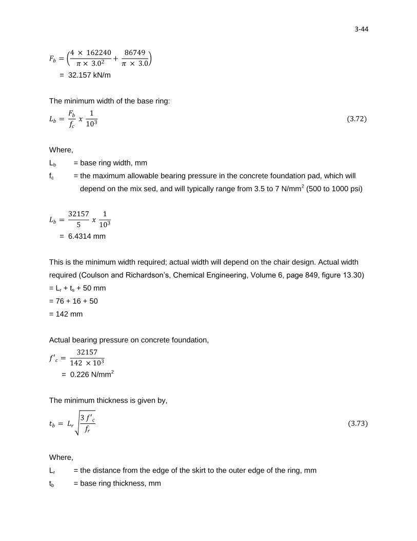
The minimum width of the base ring:
𝐿𝑏 = 𝐹𝑏
𝑓𝑐 𝑥
1
103 (3.72)
Where,
Lb = base ring width, mm
fc = the maximum allowable bearing pressure in the concrete foundation pad, which will
depend on the mix sed, and will typically range from 3.5 to 7 N/mm2 (500 to 1000 psi)
𝐿𝑏 = 32157
5 𝑥
1
103
= 6.4314 mm
This is the minimum width required; actual width will depend on the chair design. Actual width
required (Coulson and Richardson’s, Chemical Engineering, Volume 6, page 849, figure 13.30)
= Lr + ts + 50 mm
= 76 + 16 + 50
= 142 mm
Actual bearing pressure on concrete foundation,
𝑓′𝑐 = 32157
142 × 103
= 0.226 N/mm2
The minimum thickness is given by,
𝑡𝑏 = 𝐿𝑟 3 𝑓′𝑐𝑓𝑟
(3.73)
Where,
Lr = the distance from the edge of the skirt to the outer edge of the ring, mm
tb = base ring thickness, mm

3-45
f’c = actual bearing pressure on base, N/mm2
fr = allowable design stress in the ring material, typically 140 N/mm2
𝑡𝑏 = 76 3 × 0.226
140
= 5.29 mm
The chair dimensions from figure 13.30 for bolt size M24.
Skirt is to be welded flush with outer diameter of column shell.
3.3.10 Design of Nozzles
There are three nozzles in the distillation column, which are nozzles in feed inlet, top product
outlet and bottom product outlet. By assuming that the flow of the pipe is turbulent flow,
therefore to determine the optimum duct diameter is:
Optimum duct diameter, dopt = 293 G0.53ρ-0.37 (3.74)
Where,
G = flowrate, kg/s
ρ = density, kg/m3
The material construction used for nozzles is carbon steel pipe.
3.3.10.1 Feed Stream
G = 1.587 x 10⁴ kg/h
= 4.4083 kg/s
ρmix = 778.66 kg/m3
dopt = 293 (4.4083)0.53 (778.66)-0.37
= 54.77 mm
≈ 55 mm
𝑁𝑜𝑧𝑧𝑙𝑒 𝑡𝑖𝑐𝑘𝑛𝑒𝑠𝑠, 𝑡 = 𝑃𝑠𝑑𝑜𝑝𝑡
20𝜍 + 𝑃𝑠 3.75
3-46
Where,
Ps = operating pressure
σ = design stress at working temperature
𝑇𝑖𝑐𝑘𝑛𝑒𝑠𝑠 𝑜𝑓 𝑛𝑜𝑧𝑧𝑙𝑒: 𝑡 = 0.0902 × 54.77
20 125 + 0.0902
= 0.002 mm
So, the thickness of nozzle = corrosion allowance + 0.002
= 2 + 0.002
= 2.002 mm
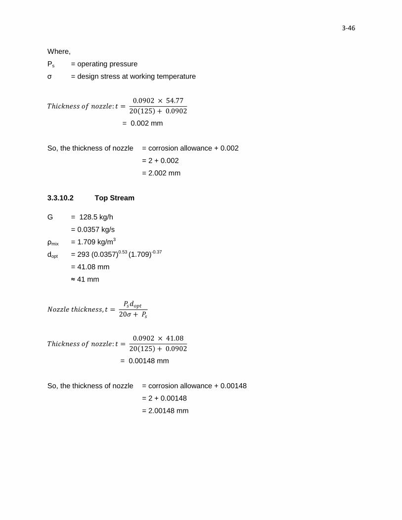
3.3.10.2 Top Stream
G = 128.5 kg/h
= 0.0357 kg/s
ρmix = 1.709 kg/m3
dopt = 293 (0.0357)0.53 (1.709)-0.37
= 41.08 mm
≈ 41 mm
𝑁𝑜𝑧𝑧𝑙𝑒 𝑡𝑖𝑐𝑘𝑛𝑒𝑠𝑠, 𝑡 = 𝑃𝑠𝑑𝑜𝑝𝑡
20𝜍 + 𝑃𝑠
𝑇𝑖𝑐𝑘𝑛𝑒𝑠𝑠 𝑜𝑓 𝑛𝑜𝑧𝑧𝑙𝑒: 𝑡 = 0.0902 × 41.08
20 125 + 0.0902
= 0.00148 mm
So, the thickness of nozzle = corrosion allowance + 0.00148
= 2 + 0.00148
= 2.00148 mm

3-47
3.3.10.3 Bottom Stream
G = 1.574 x 10⁴ kg/h
= 4.372 kg/s
ρmix = 695.2 kg/m3
dopt = 293 (4.372)0.53 (695.2)-0.37
= 56.88 mm
≈ 60 mm
𝑁𝑜𝑧𝑧𝑙𝑒 𝑡𝑖𝑐𝑘𝑛𝑒𝑠𝑠, 𝑡 = 𝑃𝑠𝑑𝑜𝑝𝑡
20𝜍 + 𝑃𝑠
𝑇𝑖𝑐𝑘𝑛𝑒𝑠𝑠 𝑜𝑓 𝑛𝑜𝑧𝑧𝑙𝑒: 𝑡 = 0.0902 × 56.88
20 125 + 0.0902
= 0.0021 mm
So, the thickness of nozzle = corrosion allowance + 0.0021
= 2 + 0.0021
= 2.0021 mm
3.3.11 Flange Design
The flange class number required for a particular duty will depend on the design pressure and
temperature and the flange material. The flange design is from the typical standard flange
design in Coulson and Richardson’s, Chemical Engineering, Volume 6, page 863, figure 13.37.
Table 3.12 The Summary of Flange Design
Feed Stream
dopt d1 Flange Raised face
Bolting Drilling Boss
D b H d4 f No d2 k d3
65 76.1 160 14 32 110 3 M12 4 14 130 100

3-48
Top Stream
dopt d1 Flange Raised face
Bolting Drilling Boss
D b H d4 f No d2 k d3
25 33.7 100 14 24 60 2 M10 4 11 75 50
Bottom Stream
dopt d1 Flange Raised face
Bolting Drilling Boss
D b H d4 f No d2 k d3
50 60.3 140 14 28 90 3 M12 4 14 110 80
3.3.12 Summary of Mechanical Design
Summary of design distillation column are shown in table below:
Table 3.13 The Summary of Mechanical Design
Pressure Vessel
Operating Pressure, Po 0.11 N/mm2
Design Pressure, P1 0.19 N/mm2
Operating Temperature 90 oC
Design Temperature 99 oC
Column Material Carbon Steel
Safety Factor 10%
Design Stress 115 N/mm2
Head and Closure
Types Torispherical Head
Crown Radius, Rc 1.128 m
Knuckle Radius, Rk 0.0677 m
Joint Factor, J 1
Cs 1.77
Minimum thickness, e 10 mm
Column Weight
Dead weight of Vessel, Wv 10.52 kN
Weight of Plates, Wp 32.384 kN

3-49
Weight of Insulation, W i 5.424 kN
Total Weight, Wt 53.752 kN
Wind Speed, Uw 160 km/h
Bending Moment, Mx 210.0429 kN/m
Insulation Material Mineral Wool
Insulation Thickness 75 mm
Skirt Support
Type of Support Straight Cylindrical Skirt
Material of Construction Carbon Steel
Young’s Modulus 200,000 N/mm2
Approximate Weight, Wapprox 152.092 kN
Total Weight 205.844 kN
Bending Moment, Mx 328.2 kNm
Skirt Thickness, ts 9 mm
Skirt Height, Hs 4 m
Stiffness Ring
Critical Buckling Pressure for Ring, Pc 140 N/mm2

3-50
3.4 Costing for Distillation Column
The purchased cost of the equipment is calculated using equation below (Turton et al., Analysis,
Synthesis, and Design of Chemical Processess, 3rd Edition, page 906):
log10 Cp° = K1 + K2 log10 (A) + K3 [log10 (A)]2 (1.0)
where,
A = capacity or size parameter for the equipment
K1, K2, K3 = constants in Table A.1 (Appendix A)
3.4.1 Process Vessels
Column height = 13 m; Column diameter = 1.33 m
Material of construction = carbon steel with stainless steel cladding
Volume = 𝜋𝐷2
= (3.142)(1.33)2(13)
= 72.25m3
From Table A.1 (Appendix A), K1 = 3.4974, K2 = 0.4485, K3 = 0.1074
log10 Cp° = 3.4974 + 0.4485 log10 (72.25) + 0.1074 [log10 (72.25)]2
= 4.73
Cp° = $ 53 751.28
Pressure factors for process vessels:
For pressure vessel, when ,003.0 mtvessel

3-51
𝐹𝑃,𝑣𝑒𝑠𝑠𝑒𝑙 =
𝑃 + 1 𝐷2[850 − 0.6 𝑃 + 1 ]
+ 0.00315
0.003 (2.0)
𝐹𝑃,𝑣𝑒𝑠𝑠𝑒𝑙 =
0.0902 + 1 (1.33)2[850 − 0.6 0.0902 + 1 ]
+ 0.00315
0.003
𝐹𝑝 ,𝑣𝑒𝑠𝑠𝑒𝑙 = 8.96 × 10⁻⁴
The bare module factor for process vessel (Turton et al., Analysis, Synthesis, and Design of
Chemical Processess, 3rd Edition, page 927):
CBM = Cp°FBM = Cp
°(B1 + B2FMFp) (3.0)
From Table A.4 (Appendix A), B1 = 2.25, B2 = 1.82
From Table A.3 (Appendix A), the identification number for carbon steel vertical process vessels
is 18.
Hence, from Figure A.18 (Appendix A), material factor, FM = 1.0
CBM = 53751.28 [2.25 + (1.82)(1.0)(8.96×10⁻⁴)]
= $ 121 028.03
Use correlation:
CEPCI for year of 2009 is 645.5
CEPCI for year of 2001 is 397
Therefore,

3-52
𝑛𝑒𝑤 𝐶𝐵𝑀 = 121 028.03 ×645.5
297
= $ 263042.40
= RM 802 279.32
3.4.2 Sieve Tray
Column height = 13 m; Column diameter = 1.33 m, Area = 5.56 m2; Number of trays = 24
From Table A.1 (Appendix A), K1 = 2.9949, K2 = 0.4465, K3 = 0.3961
log10 Cp° = 2.9949+ 0.4465 log10 (5.56) + 0.3961 [log10 (5.56)]2
= 3.92
Cp° = $ 8 275.15
The bare module cost for sieve trays (Turton et al., Analysis, Synthesis, and Design of Chemical
Processess, 3rd Edition, page 930, Table A.5):
CBM = Cp°NFBMFq (4.0)
Where,
N = number of trays
Fq = quantity factor for trays
For N≥ 20, Fq = 1
From Table A.6 (Appendix A), the identification number for stainless steel sieve trays is 61
Hence, from Figure A.19 (Appendix A), bare module factor, FBM = 1.8

3-53
CBM = (8275.15)(24)(1.8)(1)
= $ 208 533.79
Use correlation:
CEPCI for year of 2010 is 645.5
CEPCI for year of 2001 is 397
Therefore,
𝑛𝑒𝑤 𝐶𝐵𝑀 = 208 533.79 ×645.5
297
= $ 453 227.48
= RM 1 382 343.81
Thus, the total cost for distillation column = RM 802 279.32 + RM 1 382 343.81
= RM 2 184 623.13

3-54
REFERENCES
R. K. Sinnot. 2003. Chemical Engineering Design. Vol 6, 3rd Ed, Elsevier Butterworth
Heinemann.
Felder, R. M. & Rousseau, R. W. 2000. Elementary Principles of Chemical Processes. 3rd Ed,
John Wiley & Sons, Inc.
Levenspiel, O. 1999. Chemical Reaction Engineering. 3rd. Ed, John Wiley & Sons, Inc.
Perry, R. H. & Green, D. W. 1998. Perry’s Chemical Engineer’s Handbook. 7th Ed, McGraw-Hill
International Edition.
Walas, S. M. 1988. Chemical Process Equipment. Butterworths Publishers.
Ludwig, E. E. 1995. Applied Process Design. Vol.2, 3rd. Ed, Gulf Publishing Company.