Chapter 3. Discrete Random Variablesand Their Probability Distributions

2.11 Definition of random variable

3.1 Definition of a discrete random variable

3.2 Probability distribution of a discrete ran-dom variable

3.3 Expected value of a random variable or afunction of a random variable

3.4-3.8 Well-known discrete probability distri-butions

Discrete uniform probability distribution

Bernoulli probability distribution

Binomial probability distribution

Geometric probability distribution

Hypergeometric probability distribution

Poisson probability distribution

3.9 Moments and Moment generating func-tions (see Chapter 6)

3.11 Tchebysheff’s Theorem

1

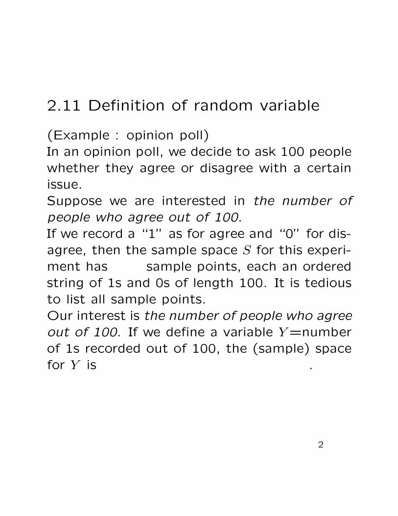
2.11 Definition of random variable

(Example : opinion poll)In an opinion poll, we decide to ask 100 peoplewhether they agree or disagree with a certainissue.Suppose we are interested in the number ofpeople who agree out of 100.If we record a “1” as for agree and “0” for dis-agree, then the sample space S for this experi-ment has 2100 sample points, each an orderedstring of 1s and 0s of length 100. It is tediousto list all sample points.Our interest is the number of people who agreeout of 100. If we define a variable Y=numberof 1s recorded out of 100, the (sample) spacefor Y is the set of integers {0,1,...,100}.

2

It frequently occurs that we are mainly inter-ested in some functions of the outcomes asopposed to the outcome itself. In the exam-ple what we do is to define a new variable Y ,the quantity of our interest. In statistics, Y iscalled a random variable.

(Def 2.12) A random variable (RV) Y is a real-valued function(mapping) from S into (not onto)R, a set of real number,

Y : S → R where y = Y (s) and s ∈ S.[note]

• Use late-alphabet capital letters (e.g., X, Y , Z) forRVs

• The support of Y is the set of possible values of Y ,{y ∈ R : Y (s) = y, s ∈ S}.

• The different roles of (capital) Y and (lowercase)y(=a particular value that a RV Y may assume).

(Example) Toss of a coin1) What is the S?2) We are interested in Y = number of tail.What is the support of Y ?3) Y : S → R

3

[Note] Y : S → R where y = Y (s) and s ∈ S.

• Y is a variable that is a function of thesample points in S.

• Mapping or function: For each s ∈ S, thereexists one and only one y such that y =Y (s) :

• One assigns a real number denoting thevalue of Y to each point in S :{Y = y} = {s : Y (s) = y, s ∈ S} is thenumerical event assigned the number y.

• Y partitions S into subsets so that pointswithin a subset are all assigned the samevalue of Y . These subsets are mutually ex-clusive since no point is assigned two dif-ferent numerical values.

• P (Y = y) is the sum of the probabilitiesof the sample points that are assigned thevalue y.

4

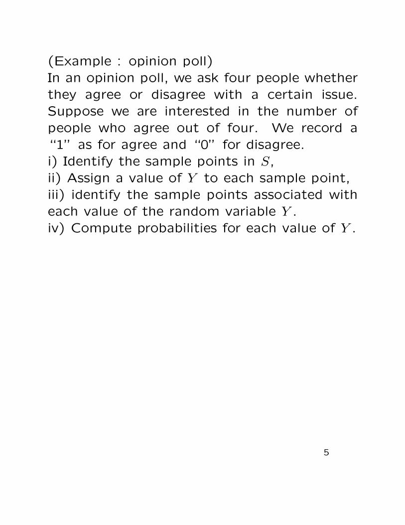
(Example : opinion poll)In an opinion poll, we ask four people whetherthey agree or disagree with a certain issue.Suppose we are interested in the number ofpeople who agree out of four. We record a“1” as for agree and “0” for disagree.i) Identify the sample points in S,ii) Assign a value of Y to each sample point,iii) identify the sample points associated witheach value of the random variable Y .iv) Compute probabilities for each value of Y .

5

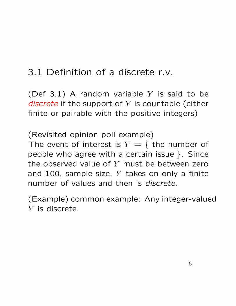
3.1 Definition of a discrete r.v.

(Def 3.1) A random variable Y is said to bediscrete if the support of Y is countable (eitherfinite or pairable with the positive integers)

(Revisited opinion poll example)The event of interest is Y = { the number ofpeople who agree with a certain issue }. Sincethe observed value of Y must be between zeroand 100, sample size, Y takes on only a finitenumber of values and then is discrete.

(Example) common example: Any integer-valuedY is discrete.

6

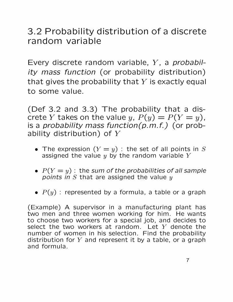
3.2 Probability distribution of a discreterandom variable

Every discrete random variable, Y , a probabil-ity mass function (or probability distribution)that gives the probability that Y is exactly equalto some value.

(Def 3.2 and 3.3) The probability that a dis-crete Y takes on the value y, P (y) = P (Y = y),is a probability mass function(p.m.f.) (or prob-ability distribution) of Y

• The expression (Y = y) : the set of all points in Sassigned the value y by the random variable Y

• P (Y = y) : the sum of the probabilities of all samplepoints in S that are assigned the value y

• P (y) : represented by a formula, a table or a graph

(Example) A supervisor in a manufacturing plant hastwo men and three women working for him. He wantsto choose two workers for a special job, and decides toselect the two workers at random. Let Y denote thenumber of women in his selection. Find the probabilitydistribution for Y and represent it by a table, or a graphand formula.

7

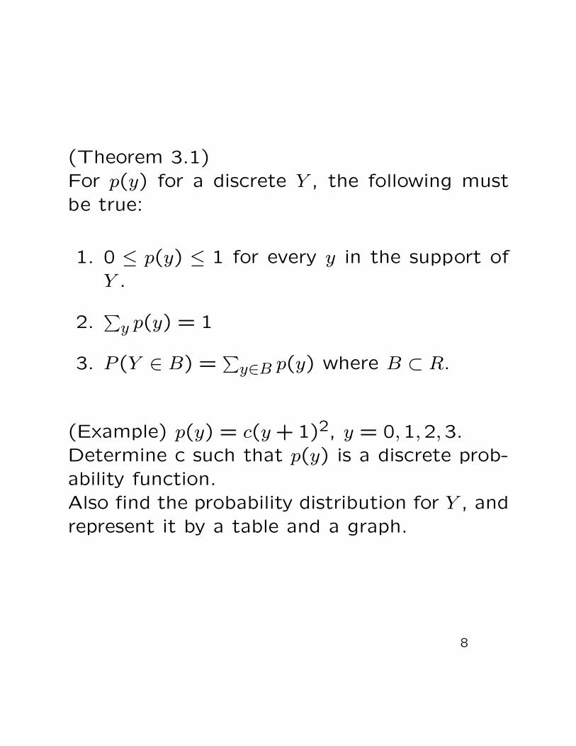
(Theorem 3.1)For p(y) for a discrete Y , the following mustbe true:

1. 0 ≤ p(y) ≤ 1 for every y in the support ofY .

2.∑y p(y) = 1

3. P (Y ∈ B) =∑y∈B p(y) where B ⊂ R.

(Example) p(y) = c(y + 1)2, y = 0,1,2,3.Determine c such that p(y) is a discrete prob-ability function.Also find the probability distribution for Y , andrepresent it by a table and a graph.

8

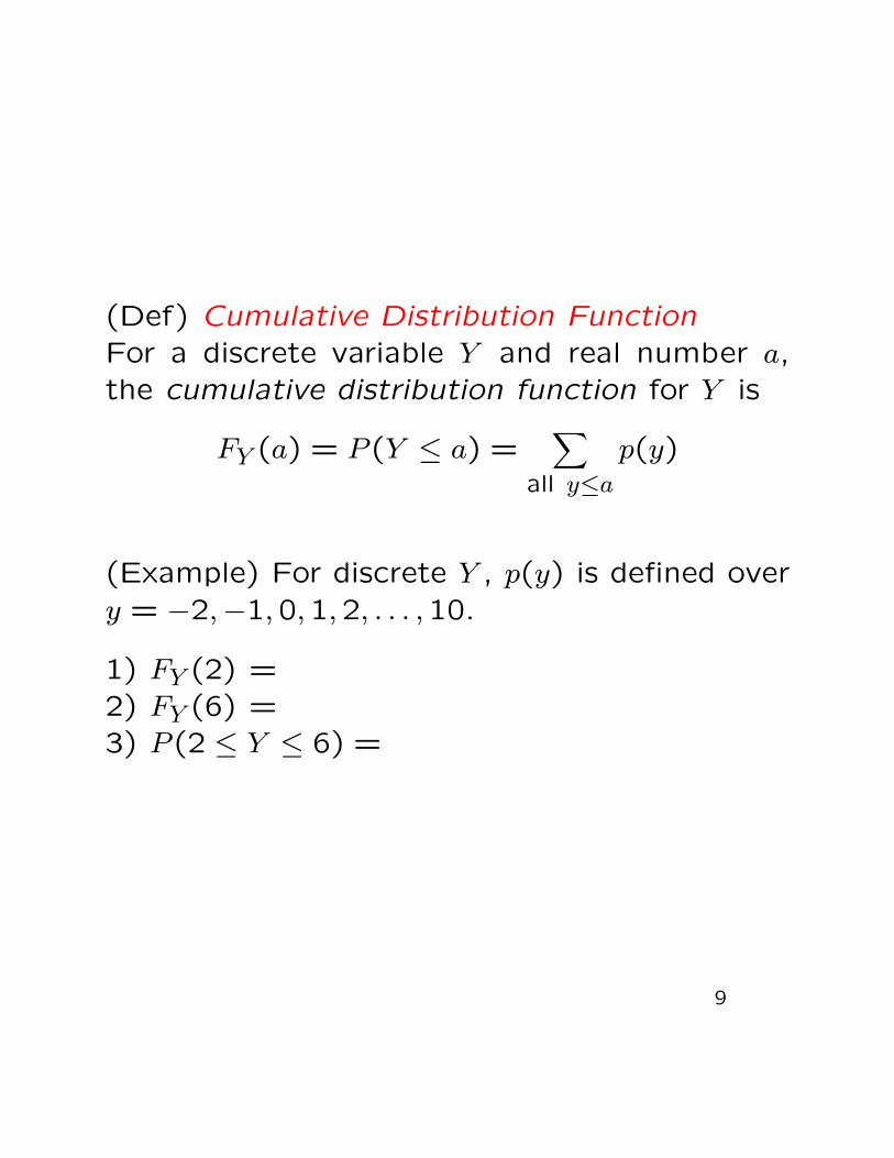
(Def) Cumulative Distribution FunctionFor a discrete variable Y and real number a,the cumulative distribution function for Y is

FY (a) = P (Y ≤ a) =∑

all y≤ap(y)

(Example) For discrete Y , p(y) is defined overy = −2,−1,0,1,2, . . . ,10.

1) FY (2) =2) FY (6) =3) P (2 ≤ Y ≤ 6) =

9

3.3 The expected value of a r.v. or afunction of a r.v.

The probability distribution for a r.v. Y : the-oretical model for real distribution of data as-sociated with a real population.

[Note] Given n observed samples y1, . . . , yn, how one candescribe the distribution of the data?

• measures of central tendency

– Sample mean, y = 1n

∑ni=1 yi for the unknown

population mean : µ

• measures of dispersion or variation

– Sample variance, s2 = 1n−1

∑ni=1(yi − y)2 and

Sample standard deviation, s =√s2 for the un-

known population variance and standard devia-tion: σ2 and σ

Our interest : characteristics of the probabilitydistribution (p.m.f.) p(y) for a discrete Y suchas the mean and the variance for a discrete Y .

10

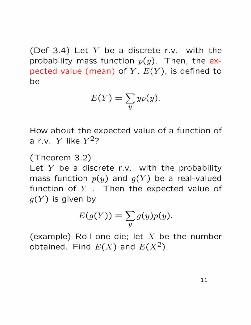
(Def 3.4) Let Y be a discrete r.v. with theprobability mass function p(y). Then, the ex-pected value (mean) of Y , E(Y ), is defined tobe

E(Y ) =∑yyp(y).

How about the expected value of a function ofa r.v. Y like Y 2?

(Theorem 3.2)Let Y be a discrete r.v. with the probabilitymass function p(y) and g(Y ) be a real-valuedfunction of Y . Then the expected value ofg(Y ) is given by

E(g(Y )) =∑yg(y)p(y).

(example) Roll one die; let X be the numberobtained. Find E(X) and E(X2).

11

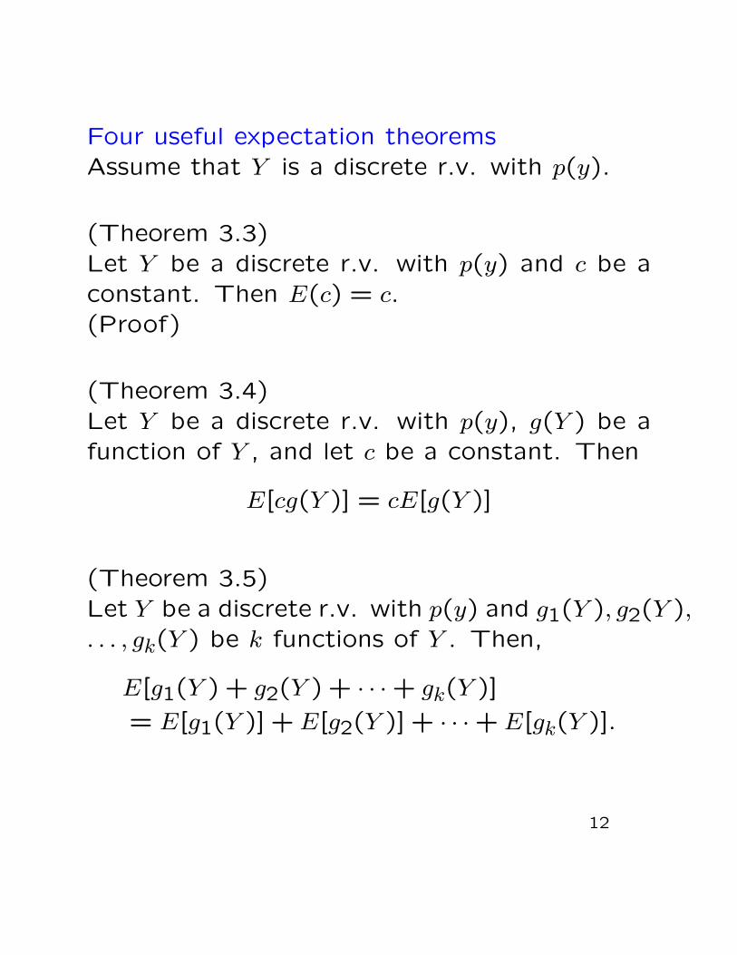
Four useful expectation theoremsAssume that Y is a discrete r.v. with p(y).

(Theorem 3.3)Let Y be a discrete r.v. with p(y) and c be aconstant. Then E(c) = c.(Proof)

(Theorem 3.4)Let Y be a discrete r.v. with p(y), g(Y ) be afunction of Y , and let c be a constant. Then

E[cg(Y )] = cE[g(Y )]

(Theorem 3.5)Let Y be a discrete r.v. with p(y) and g1(Y ), g2(Y ),. . . , gk(Y ) be k functions of Y . Then,

E[g1(Y ) + g2(Y ) + · · ·+ gk(Y )]

= E[g1(Y )] + E[g2(Y )] + · · ·+ E[gk(Y )].

12

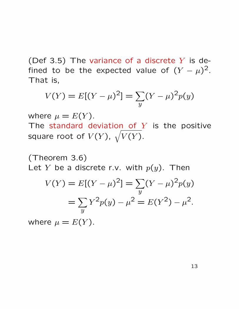
(Def 3.5) The variance of a discrete Y is de-fined to be the expected value of (Y − µ)2.That is,

V (Y ) = E[(Y − µ)2] =∑y

(Y − µ)2p(y)

where µ = E(Y ).The standard deviation of Y is the positive

square root of V (Y ),√V (Y ).

(Theorem 3.6)Let Y be a discrete r.v. with p(y). Then

V (Y ) = E[(Y − µ)2] =∑y

(Y − µ)2p(y)

=∑yY 2p(y)− µ2 = E(Y 2)− µ2.

where µ = E(Y ).

13

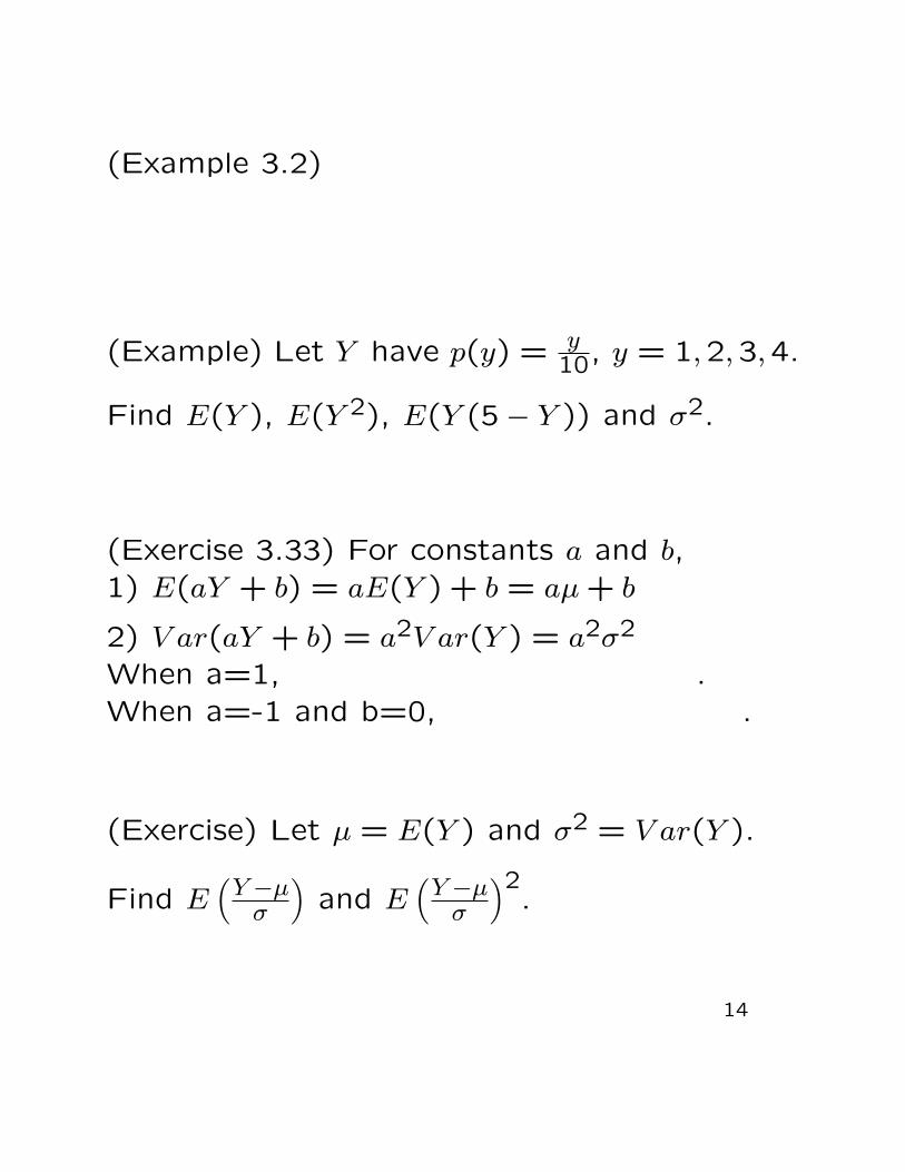
(Example 3.2)

(Example) Let Y have p(y) = y10, y = 1,2,3,4.

Find E(Y ), E(Y 2), E(Y (5− Y )) and σ2.

(Exercise 3.33) For constants a and b,1) E(aY + b) = aE(Y ) + b = aµ+ b

2) V ar(aY + b) = a2V ar(Y ) = a2σ2

When a=1, .When a=-1 and b=0, .

(Exercise) Let µ = E(Y ) and σ2 = V ar(Y ).

Find E(Y−µσ

)and E

(Y−µσ

)2.

14

In practice many experiments exhibit similar characteris-tics and generate random variables with the same typesof probability distribution.

It is important to know the probability distributions,means and variances for random variables associatedwith common types of experiments.

Note that a probability distribution for a r.v. Y has the(unknown) constant(s) that determine its specific form,called parameters.

3.4-1 The discrete uniform random vari-able

(Def) A random variable Y is said to have a dis-crete uniform distribution with the parameterm if and only if p(y) = 1

m where y = 1,2, . . . ,m.

(Theorem) Let Y be a discrete uniform randomvariable. Then,

µ = E(Y ) =m+ 1

2and σ2 = V (Y ) =

m2 − 1

12.

(Question) Does p(y) in (Def) above satisfythe necessary properties in (Theorem 3.1)?

15

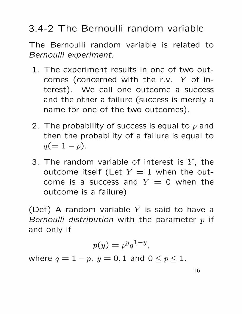
3.4-2 The Bernoulli random variable

The Bernoulli random variable is related toBernoulli experiment.

1. The experiment results in one of two out-comes (concerned with the r.v. Y of in-terest). We call one outcome a successand the other a failure (success is merely aname for one of the two outcomes).

2. The probability of success is equal to p andthen the probability of a failure is equal toq(= 1− p).

3. The random variable of interest is Y , theoutcome itself (Let Y = 1 when the out-come is a success and Y = 0 when theoutcome is a failure)

(Def) A random variable Y is said to have aBernoulli distribution with the parameter p ifand only if

p(y) = pyq1−y,

where q = 1− p, y = 0,1 and 0 ≤ p ≤ 1.

16

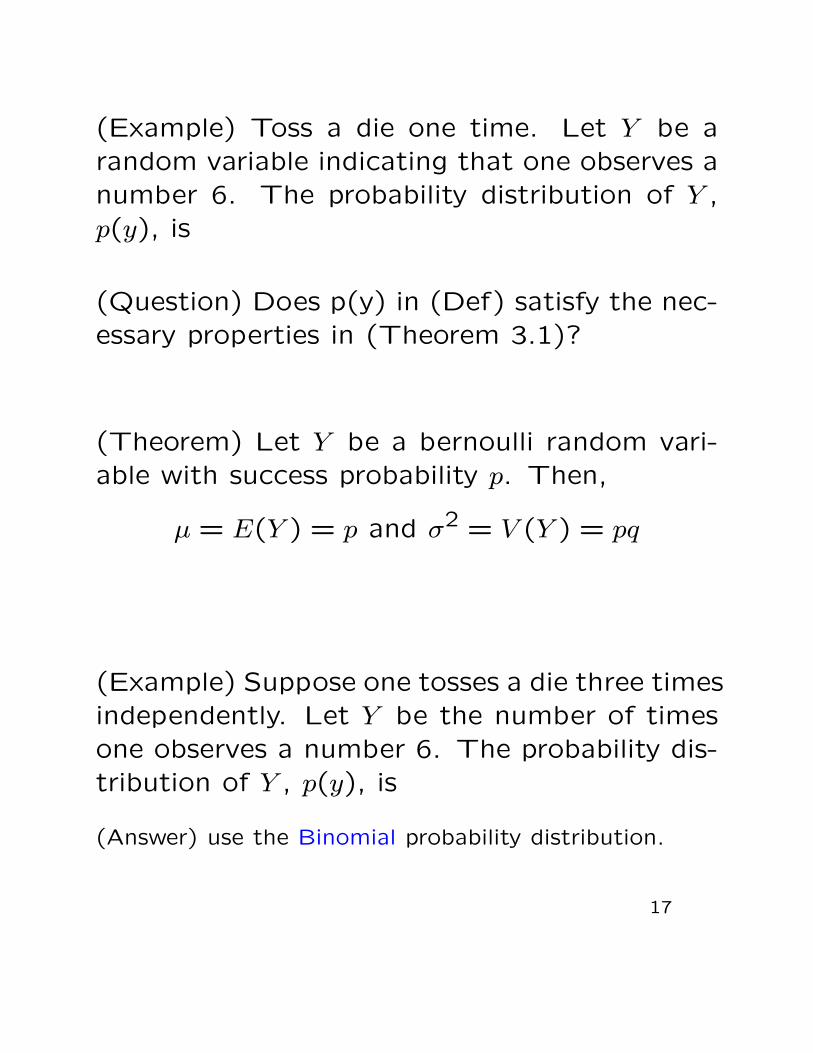
(Example) Toss a die one time. Let Y be arandom variable indicating that one observes anumber 6. The probability distribution of Y ,p(y), is

(Question) Does p(y) in (Def) satisfy the nec-essary properties in (Theorem 3.1)?

(Theorem) Let Y be a bernoulli random vari-able with success probability p. Then,

µ = E(Y ) = p and σ2 = V (Y ) = pq

(Example) Suppose one tosses a die three timesindependently. Let Y be the number of timesone observes a number 6. The probability dis-tribution of Y , p(y), is

(Answer) use the Binomial probability distribution.

17

3.4-3 The Binomial random variable

The Binomial random variable is related to bi-nomial experiments

(Def 3.6)

1. The experiment consists of n identical and indepen-dent trials.

2. Each trial results in one of two outcomes (con-cerned with the r.v. Y of interest). We call oneoutcome a success S and the other a failure F .Here, success is merely a name for one of the twopossible outcomes on a single trial of an experiment.

3. The probability of success on a single trial is equalto p and remains the same from trial to trial. Theprobability of a failure is equal to q(= 1− p).

4. The random variable of interest is Y , the number

of successes observed during the n trials.

(Example 3.5) Reading

18

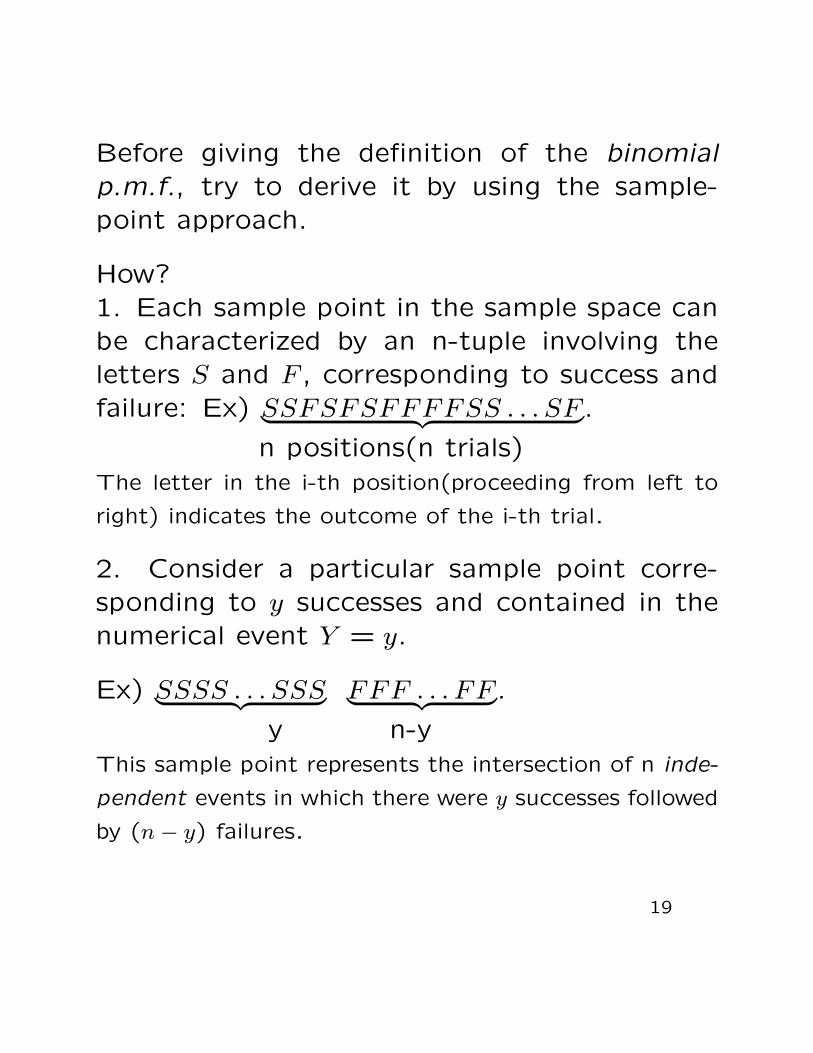
Before giving the definition of the binomialp.m.f., try to derive it by using the sample-point approach.

How?1. Each sample point in the sample space canbe characterized by an n-tuple involving theletters S and F , corresponding to success andfailure: Ex) SSFSFSFFFFSS . . . SF︸ ︷︷ ︸.

n positions(n trials)The letter in the i-th position(proceeding from left to

right) indicates the outcome of the i-th trial.

2. Consider a particular sample point corre-sponding to y successes and contained in thenumerical event Y = y.

Ex) SSSS . . . SSS︸ ︷︷ ︸ FFF . . . FF︸ ︷︷ ︸.y n-y

This sample point represents the intersection of n inde-

pendent events in which there were y successes followed

by (n− y) failures.

19

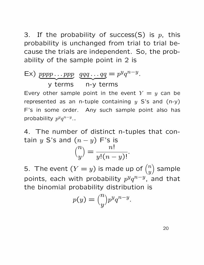
3. If the probability of success(S) is p, thisprobability is unchanged from trial to trial be-cause the trials are independent. So, the prob-ability of the sample point in 2 is

Ex) pppp . . . ppp︸ ︷︷ ︸ qqq . . . qq︸ ︷︷ ︸ = pyqn−y.

y terms n-y termsEvery other sample point in the event Y = y can be

represented as an n-tuple containing y S’s and (n-y)

F’s in some order. Any such sample point also has

probability pyqn−y..

4. The number of distinct n-tuples that con-tain y S’s and (n− y) F’s is(n

y

)=

n!

y!(n− y)!.

5. The event (Y = y) is made up of(ny

)sample

points, each with probability pyqn−y, and thatthe binomial probability distribution is

p(y) =(ny

)pyqn−y.

20

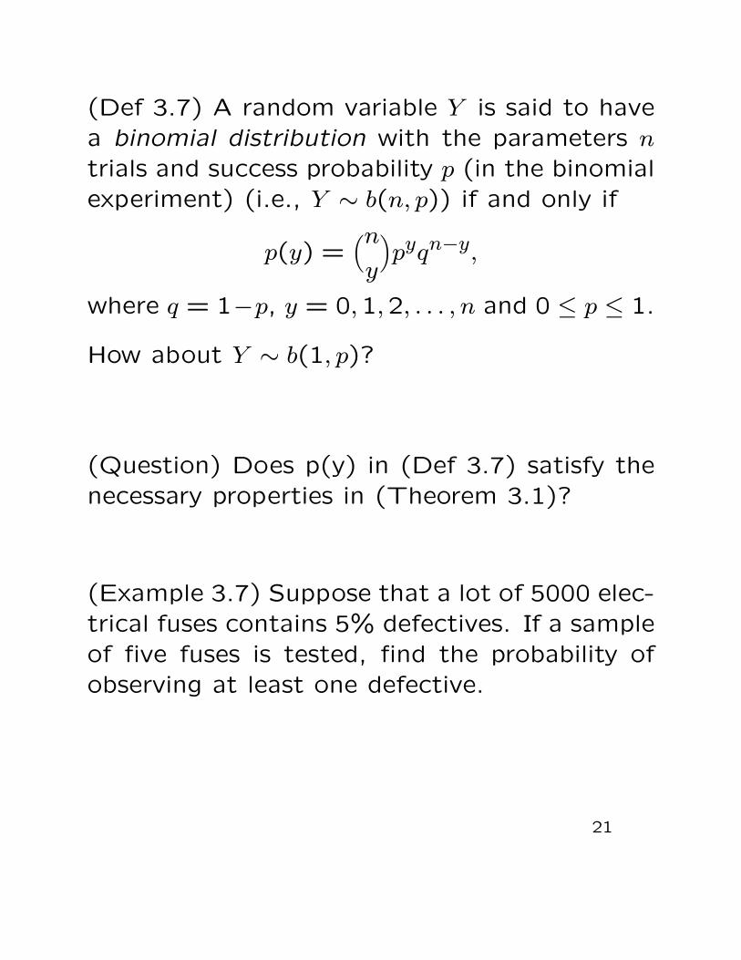
(Def 3.7) A random variable Y is said to havea binomial distribution with the parameters n

trials and success probability p (in the binomialexperiment) (i.e., Y ∼ b(n, p)) if and only if

p(y) =(ny

)pyqn−y,

where q = 1−p, y = 0,1,2, . . . , n and 0 ≤ p ≤ 1.

How about Y ∼ b(1, p)?

(Question) Does p(y) in (Def 3.7) satisfy thenecessary properties in (Theorem 3.1)?

(Example 3.7) Suppose that a lot of 5000 elec-trical fuses contains 5% defectives. If a sampleof five fuses is tested, find the probability ofobserving at least one defective.

21

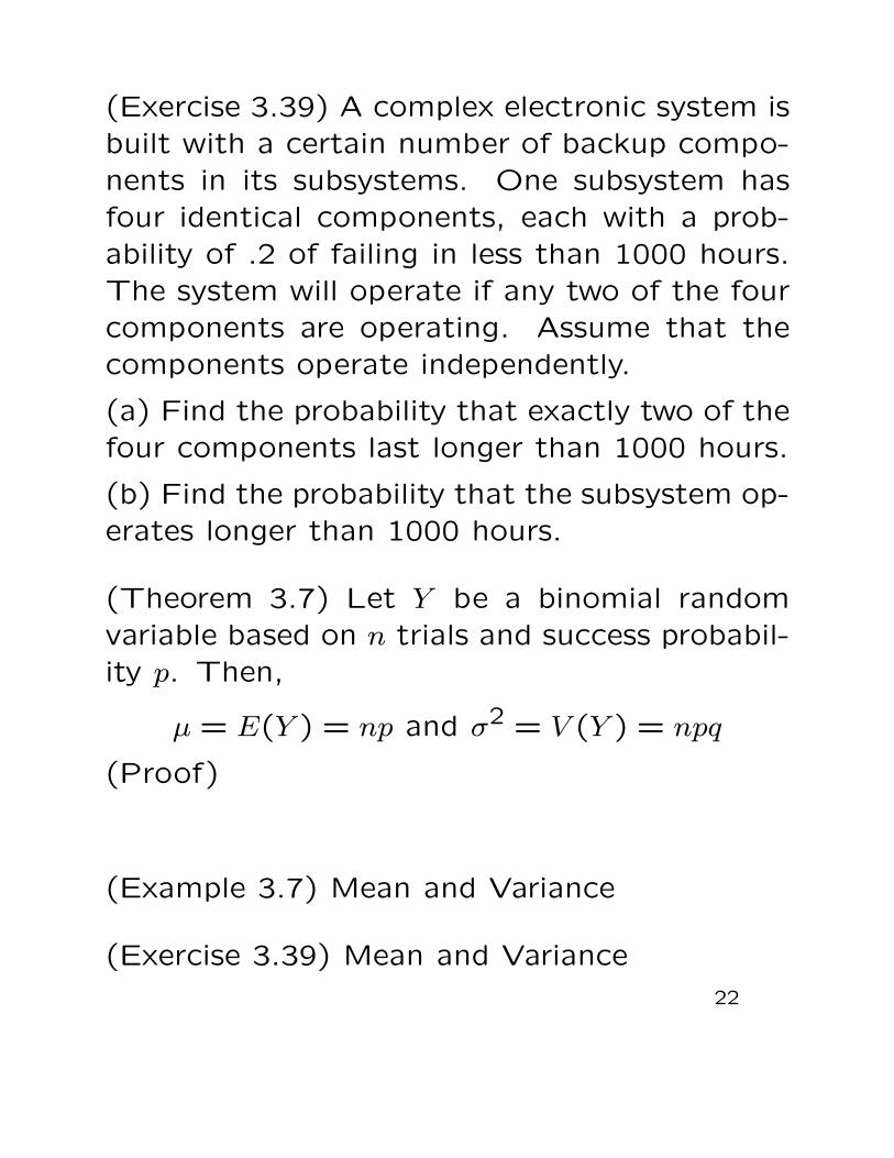
(Exercise 3.39) A complex electronic system isbuilt with a certain number of backup compo-nents in its subsystems. One subsystem hasfour identical components, each with a prob-ability of .2 of failing in less than 1000 hours.The system will operate if any two of the fourcomponents are operating. Assume that thecomponents operate independently.

(a) Find the probability that exactly two of thefour components last longer than 1000 hours.

(b) Find the probability that the subsystem op-erates longer than 1000 hours.

(Theorem 3.7) Let Y be a binomial randomvariable based on n trials and success probabil-ity p. Then,

µ = E(Y ) = np and σ2 = V (Y ) = npq

(Proof)

(Example 3.7) Mean and Variance

(Exercise 3.39) Mean and Variance

22

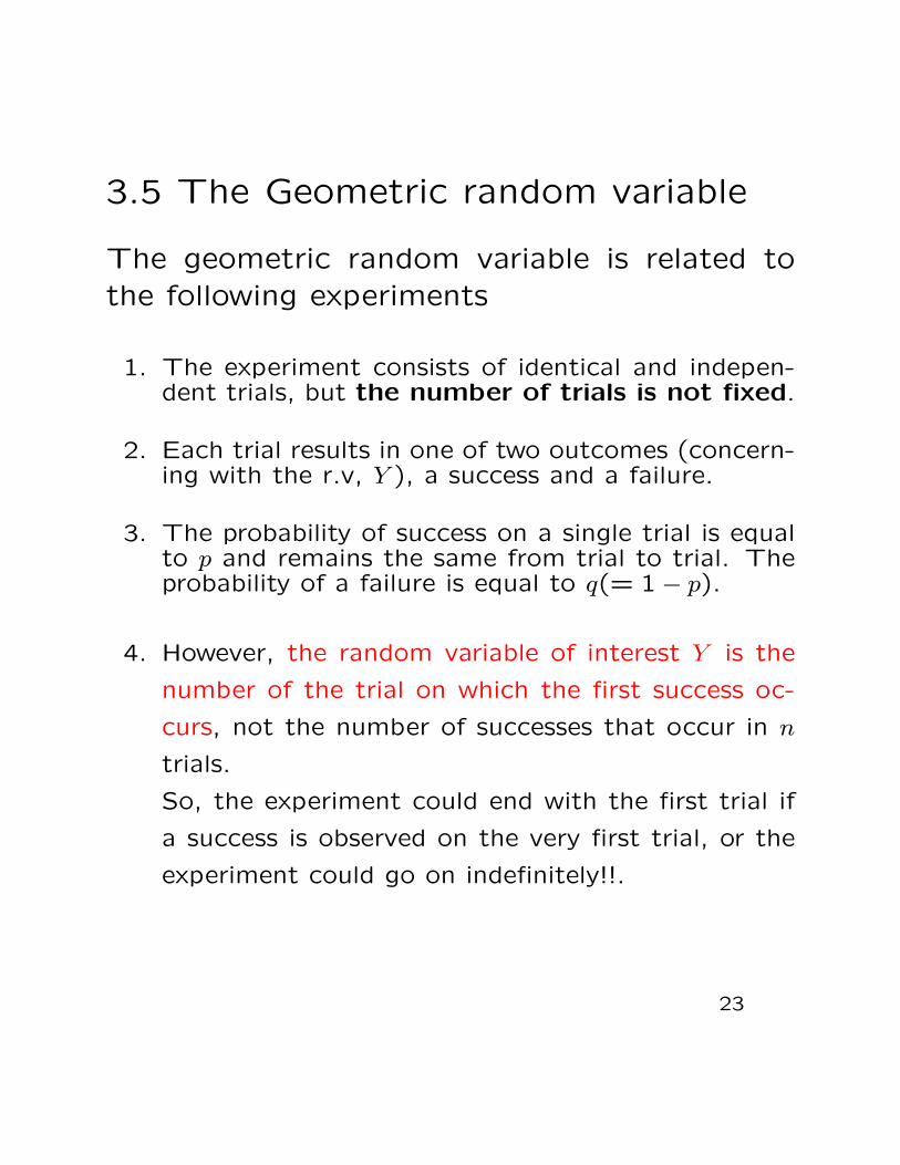
3.5 The Geometric random variable

The geometric random variable is related tothe following experiments

1. The experiment consists of identical and indepen-dent trials, but the number of trials is not fixed.

2. Each trial results in one of two outcomes (concern-ing with the r.v, Y ), a success and a failure.

3. The probability of success on a single trial is equalto p and remains the same from trial to trial. Theprobability of a failure is equal to q(= 1− p).

4. However, the random variable of interest Y is the

number of the trial on which the first success oc-

curs, not the number of successes that occur in n

trials.

So, the experiment could end with the first trial if

a success is observed on the very first trial, or the

experiment could go on indefinitely!!.

23

(Def 3.8) A random variable Y is said to have ageometric probability distribution with the pa-rameter p, success probability (i.e., Y ∼ Geo(p))if and only if

p(y) = qy−1p,

where q = 1− p, y = 1,2,3 . . . , and 0 ≤ p ≤ 1.

(Question) Does p(y) in (Def 3.8) satisfy the necessaryproperties in (Theorem 3.1)?

(Exercise 3.67) Suppose that 30% of the applicants for acertain industrial job possess advanced training in com-puter programming. Applicants are interviewed sequen-tially and are selected at random from the pool. Findthe probability that the first applicant with advancedtraining in programming is found on the fifth interview.

(Example) A basket player can make a free throw 60% ofthe time. Let X be the minimum number of free throwsthat this player must attempt to make first shot. Whatis P (X = 5)?

24

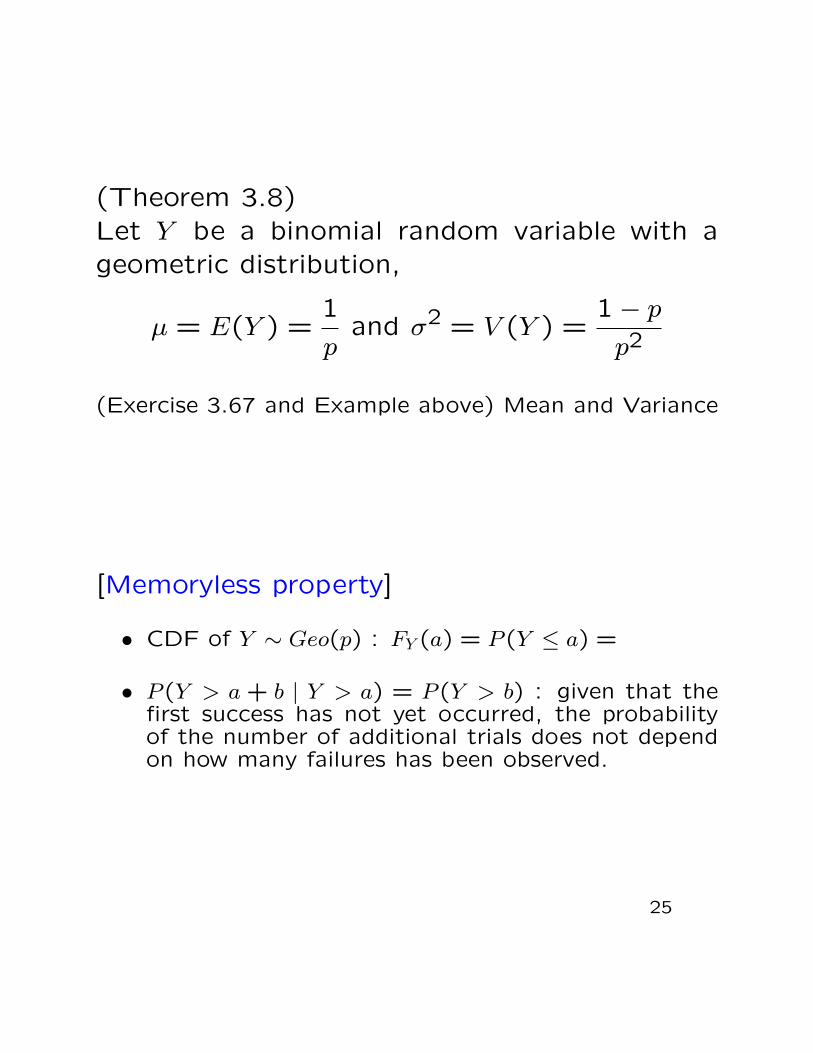
(Theorem 3.8)Let Y be a binomial random variable with ageometric distribution,

µ = E(Y ) =1

pand σ2 = V (Y ) =

1− pp2

(Exercise 3.67 and Example above) Mean and Variance

[Memoryless property]

• CDF of Y ∼ Geo(p) : FY (a) = P (Y ≤ a) =

• P (Y > a + b | Y > a) = P (Y > b) : given that thefirst success has not yet occurred, the probabilityof the number of additional trials does not dependon how many failures has been observed.

25

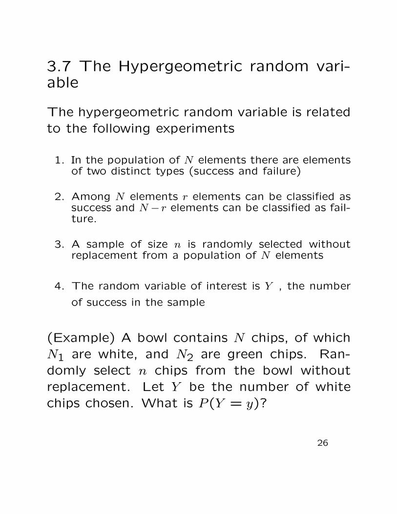
3.7 The Hypergeometric random vari-able

The hypergeometric random variable is relatedto the following experiments

1. In the population of N elements there are elementsof two distinct types (success and failure)

2. Among N elements r elements can be classified assuccess and N − r elements can be classified as fail-ture.

3. A sample of size n is randomly selected withoutreplacement from a population of N elements

4. The random variable of interest is Y , the number

of success in the sample

(Example) A bowl contains N chips, of whichN1 are white, and N2 are green chips. Ran-domly select n chips from the bowl withoutreplacement. Let Y be the number of whitechips chosen. What is P (Y = y)?

26

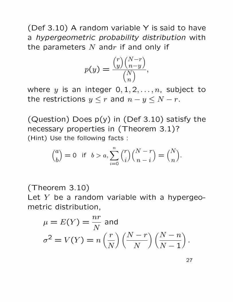
(Def 3.10) A random variable Y is said to havea hypergeometric probability distribution withthe parameters N andr if and only if

p(y) =

(ry

)(N−rn−y

)(Nn

) ,

where y is an integer 0,1,2, . . . , n, subject tothe restrictions y ≤ r and n− y ≤ N − r.

(Question) Does p(y) in (Def 3.10) satisfy thenecessary properties in (Theorem 3.1)?(Hint) Use the following facts :(a

b

)= 0 if b > a,

n∑i=0

(ri

)(N − rn− i

)=(Nn

).

(Theorem 3.10)Let Y be a random variable with a hypergeo-metric distribution,

µ = E(Y ) =nr

Nand

σ2 = V (Y ) = n

(r

N

)(N − rN

)(N − nN − 1

).

27

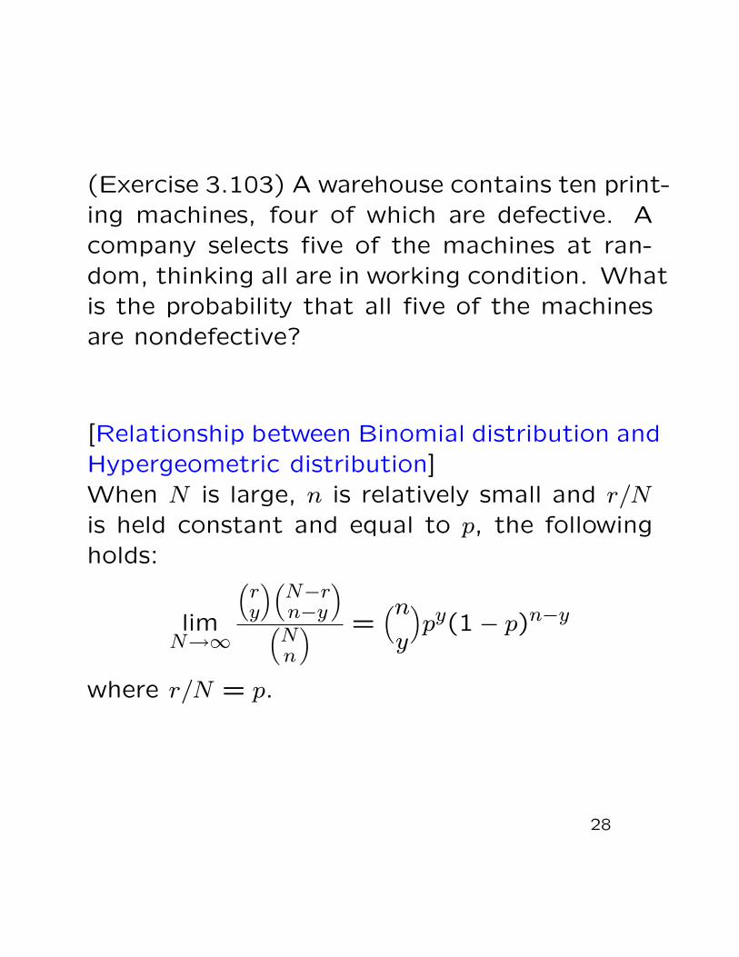
(Exercise 3.103) A warehouse contains ten print-ing machines, four of which are defective. Acompany selects five of the machines at ran-dom, thinking all are in working condition. Whatis the probability that all five of the machinesare nondefective?

[Relationship between Binomial distribution andHypergeometric distribution]When N is large, n is relatively small and r/N

is held constant and equal to p, the followingholds:

limN→∞

(ry

)(N−rn−y

)(Nn

) =(ny

)py(1− p)n−y

where r/N = p.

28

We learned the following discrete random vari-able and their probability distributions (p.m.f.):

1) Discrete uniform probability distribution

2) Bernoulli probability distribution

3) Binomial probability distribution

4) Geometric probability distribution

5) Hypergeometric probability distribution

The experiments in 2)-5) has two outcomesconcerned with the r.v. Y , for example “suc-cess“ and “failure“.

Now we will learn how to model counting data(number of times a particular event occurs) :Poisson r.v. and its probability distribution.

29

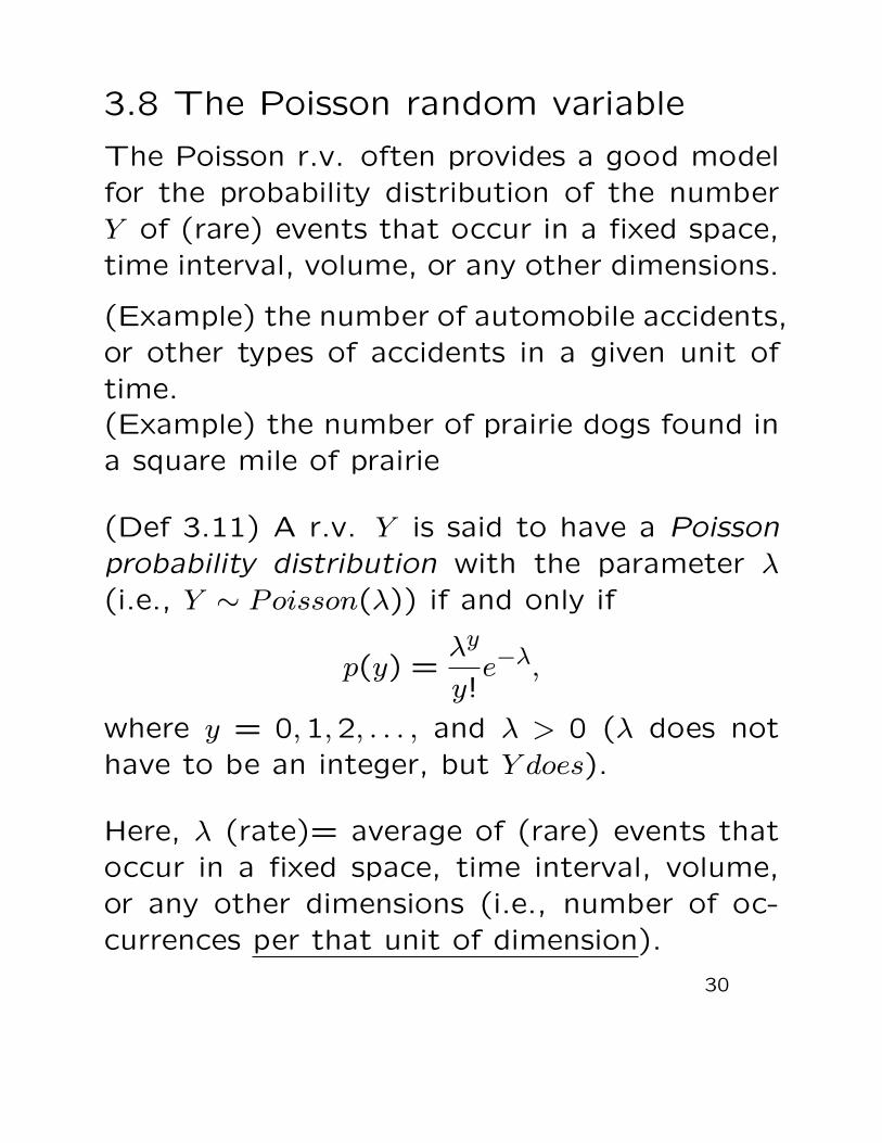
3.8 The Poisson random variable

The Poisson r.v. often provides a good modelfor the probability distribution of the numberY of (rare) events that occur in a fixed space,time interval, volume, or any other dimensions.

(Example) the number of automobile accidents,or other types of accidents in a given unit oftime.(Example) the number of prairie dogs found ina square mile of prairie

(Def 3.11) A r.v. Y is said to have a Poissonprobability distribution with the parameter λ

(i.e., Y ∼ Poisson(λ)) if and only if

p(y) =λy

y!e−λ,

where y = 0,1,2, . . . , and λ > 0 (λ does nothave to be an integer, but Y does).

Here, λ (rate)= average of (rare) events thatoccur in a fixed space, time interval, volume,or any other dimensions (i.e., number of oc-currences per that unit of dimension).

30

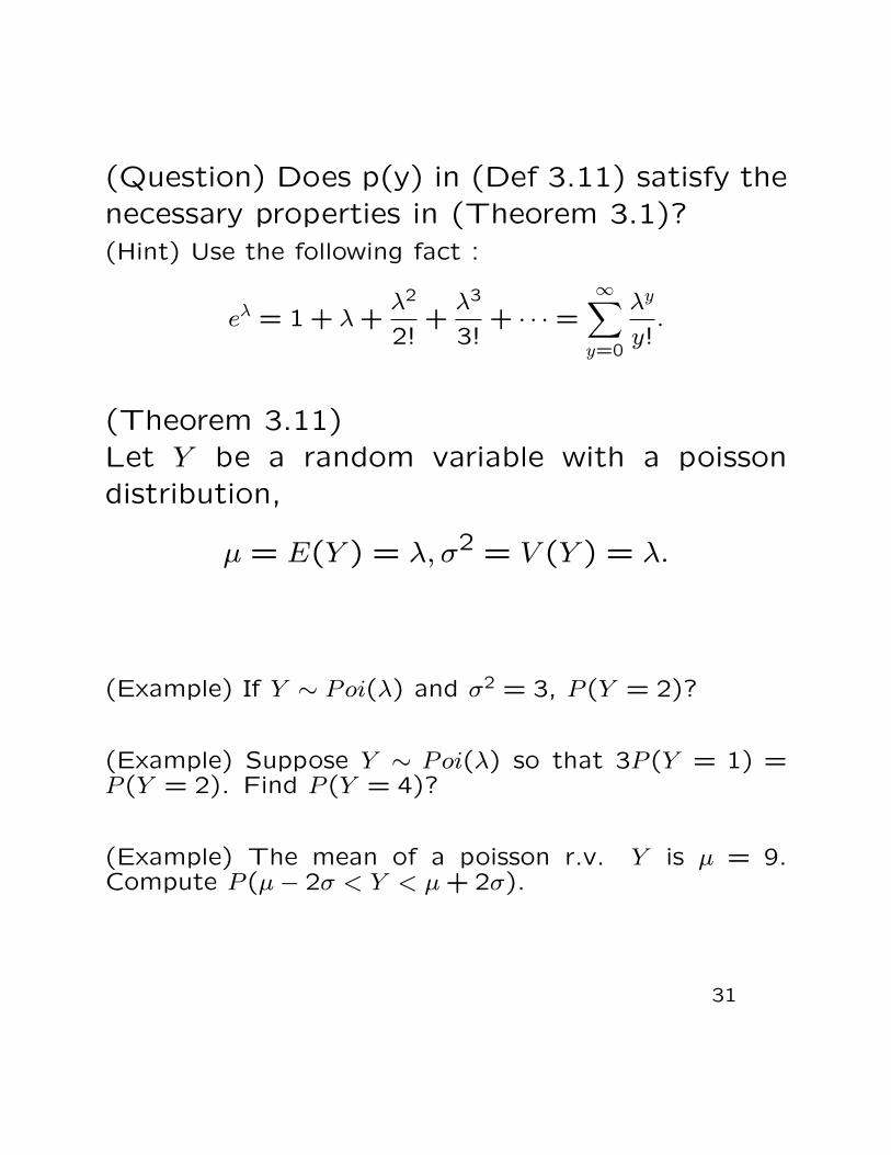
(Question) Does p(y) in (Def 3.11) satisfy thenecessary properties in (Theorem 3.1)?(Hint) Use the following fact :

eλ = 1 + λ+λ2

2!+λ3

3!+ · · · =

∞∑y=0

λy

y!.

(Theorem 3.11)Let Y be a random variable with a poissondistribution,

µ = E(Y ) = λ, σ2 = V (Y ) = λ.

(Example) If Y ∼ Poi(λ) and σ2 = 3, P (Y = 2)?

(Example) Suppose Y ∼ Poi(λ) so that 3P (Y = 1) =P (Y = 2). Find P (Y = 4)?

(Example) The mean of a poisson r.v. Y is µ = 9.Compute P (µ− 2σ < Y < µ+ 2σ).

31

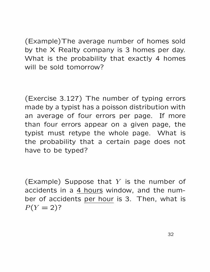
(Example)The average number of homes soldby the X Realty company is 3 homes per day.What is the probability that exactly 4 homeswill be sold tomorrow?

(Exercise 3.127) The number of typing errorsmade by a typist has a poisson distribution withan average of four errors per page. If morethan four errors appear on a given page, thetypist must retype the whole page. What isthe probability that a certain page does nothave to be typed?

(Example) Suppose that Y is the number ofaccidents in a 4 hours window, and the num-ber of accidents per hour is 3. Then, what isP (Y = 2)?

32

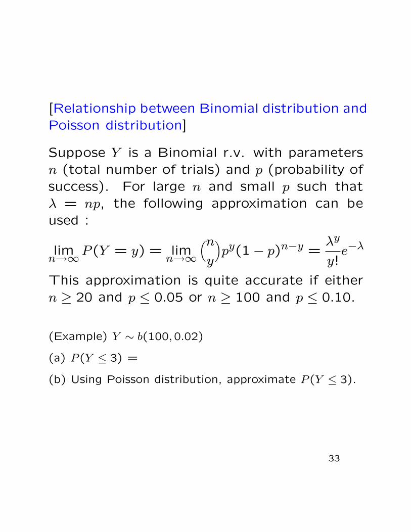
[Relationship between Binomial distribution andPoisson distribution]

Suppose Y is a Binomial r.v. with parametersn (total number of trials) and p (probability ofsuccess). For large n and small p such thatλ = np, the following approximation can beused :

limn→∞P (Y = y) = lim

n→∞

(ny

)py(1− p)n−y =

λy

y!e−λ

This approximation is quite accurate if eithern ≥ 20 and p ≤ 0.05 or n ≥ 100 and p ≤ 0.10.

(Example) Y ∼ b(100,0.02)

(a) P (Y ≤ 3) =

(b) Using Poisson distribution, approximate P (Y ≤ 3).

33

3.11 Tchebysheff’s Theorem

How one can approximate the probability thatthe r.v. Y is within a certain interval?

• Use Empirical Rule if the probability distri-bution of Y is approximately bell-shaped.

• The interval with endpoints,

· (µ − σ, µ + σ) contains approximately 68% of the measurements.

· (µ−2σ, µ+2σ) contains approximately 95% of the measurements.

· (µ − 3σ, µ + 3σ) contains approximately99.7 % of the measurements.

E.G.) suppose that the scores on STAT515 midtermexam have approximately a bell-shaped curve withµ = 80 and σ = 5. Then

· approximately 68% of the scores are between 75and 85 ,

· approximately 95% of the scores are between 70and 90,

· almost all of the scores are between 65 and 95.

34

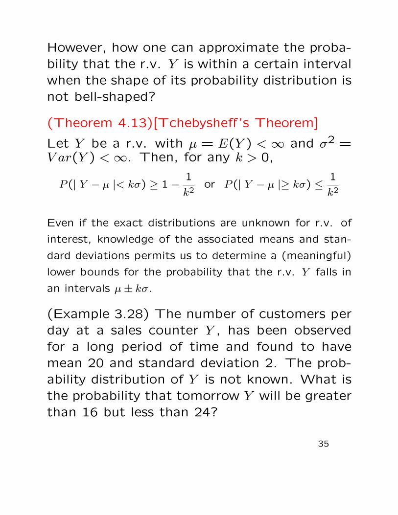
However, how one can approximate the proba-bility that the r.v. Y is within a certain intervalwhen the shape of its probability distribution isnot bell-shaped?

(Theorem 4.13)[Tchebysheff’s Theorem]

Let Y be a r.v. with µ = E(Y ) <∞ and σ2 =V ar(Y ) <∞. Then, for any k > 0,

P (| Y − µ |< kσ) ≥ 1−1

k2or P (| Y − µ |≥ kσ) ≤

1

k2

Even if the exact distributions are unknown for r.v. of

interest, knowledge of the associated means and stan-

dard deviations permits us to determine a (meaningful)

lower bounds for the probability that the r.v. Y falls in

an intervals µ± kσ.

(Example 3.28) The number of customers perday at a sales counter Y , has been observedfor a long period of time and found to havemean 20 and standard deviation 2. The prob-ability distribution of Y is not known. What isthe probability that tomorrow Y will be greaterthan 16 but less than 24?

35