EM 1110-2-605030 Jun 99

3-1

Chapter 3Development of Site-Specific Response Spectra for SeismicAnalysis of Concrete Hydraulic Structures

Section IIntroduction

3-1. Purpose and Scope

This chapter describes procedures for developing site-specific response spectra of ground motionsthroughout the United States for seismic analyses of hydraulic structures. Also covered, but in less detail,are approaches for developing acceleration time-histories of ground motions. Section I provides an over-view of the general approaches to developing site-specific response spectra, a brief discussion of factorsinfluencing earthquake ground motions, and a brief discussion of differences in ground motion charac-teristics in different regions of the United States. This is followed in Sections II and III by descriptionsof procedures for developing site-specific response spectra using deterministic and probabilisticapproaches, respectively.

3-2. General Approaches for Developing Site-Specific Response Spectra

The two general approaches for developing site-specific response spectra are the deterministic andprobabilistic approaches.

a. Deterministic approach.

(1) General. In this approach, often termed a deterministic seismic hazard analysis, or DSHA, siteground motions are deterministically estimated for a specific, selected earthquake, that is, an earthquakeof a certain size on a specific seismic source occurring at a certain distance from the site. The earthquakesize may be characterized by magnitude or by epicentral intensity. In the WUS, the practice has been touse magnitude, whereas in the EUS, both magnitude and Modified Mercalli Intensity (MMI) have beenused. However, in the EUS, magnitude is increasingly being used as the measure of earthquake size, andground motions are correspondingly being estimated using correlations with magnitude. In this manual,ground motions are estimated using relationships with magnitude. For procedures for estimating groundmotions as a function of intensity, reference should be made to the state-of-the-art publication byKrinitzsky and Chang (1987).

(2) Size and location of design earthquakes. In the deterministic approach, earthquake magnitude istypically selected to be the magnitude of the largest earthquake judged to be capable of occurring on theseismic source, i.e., MCE. The selected earthquake is usually assumed to occur on the portion of theseismic source that is closest to the site (an exception is the “random earthquake” analysis described inSection II and Appendix D). After the earthquake magnitude and distance are selected, the site groundmotions are then estimated using ground motion attenuation relationships or other techniques.Procedures for deterministically estimating earthquake ground motions are described in Section II.

b. Probabilistic approach. In the probabilistic approach, often termed a probabilistic seismichazard analysis, or PSHA, site ground motions are estimated for selected values of the probability ofground motion exceedance in a design time period or for selected values of annual frequency or returnperiod for ground motion exceedance. As an example, ground motions could be estimated for a 10

EM 1110-2-605030 Jun 99

3-2

percent probability of exceedance in 100 years or for a return period of 950 years. The probabilisticapproach thus provides an expression of potential earthquake loading in terms analogous to those usedfor other environmental loads in civil engineering design such as wind and flood loading. A probabilisticground motion assessment incorporates the frequency of occurrence of earthquakes of differentmagnitudes on the seismic sources, the uncertainty of the earthquake locations on the sources, and theground motion attenuation including its uncertainty. Section III describes the procedures forprobabilistically estimating earthquake ground motions.

3-3. Factors Affecting Earthquake Ground Motions

a. General. As stated in paragraph 1-8, It has been well-recognized that earthquake ground motionsare affected by earthquake source conditions, source- to-site transmission path properties, and site condi-tions. The source conditions include the stress drop, source depth, size of the rupture area, slipdistribution (amount and distribution of static displacement on the fault plane), rise time (time for thefault slip to complete at a given point on the fault plane), type of faulting, and rupture directivity. Thetransmission path properties include the crustal structure and the shear-wave velocity and dampingcharacteristics of the crustal rock. The site conditions include the rock properties beneath the site todepths of up to about 2 km, the local soil conditions at the site to depths of up to several hundred feet,and the topography of the site. In developing relationships for estimating ground motions, the effects ofsource, path, and site have been commonly represented in a simplified manner by earthquake magnitude,source-to-site distance, and local subsurface conditions. The important influences of these factors onground motion are summarized below.

b. Effects of earthquake magnitude and distance on ground motions.

(1) General. The effects of earthquake magnitude and distance on the amplitude of ground motionsare well known; ground motion amplitudes tend to increase with increasing magnitude and decreasingdistance. However, the effects of magnitude and source-to-site distance on relative frequency content(response spectral shape) and duration of ground motions are not as well known and therefore are brieflyreviewed below.

(2) Effects of magnitude. The Guerrero, Mexico, accelerograph array data illustrate the large effectof magnitude on the relative frequency content and duration of earthquake ground motions. TheGuerrero array has provided recordings of rock motions over a wide range of magnitudes. Figures 3-1and 3-2 show the accelerograms and the corresponding response spectra for six recordings selected byAnderson and Quaas (1988) to be approximately equally spaced in magnitude from the smallest event ofmagnitude 3.1 to the largest of magnitude 8.1. Figure 3-1 illustrates the effect of magnitude on theduration of the strong shaking part of an accelerogram; with increasing magnitude, duration rapidlyincreases. All events have epicenters about 25 km from the station, and all stations are on hard rock(Anderson and Quaas 1988). Figure 3-2 illustrates that the larger magnitude events have somewhatlarger spectral amplitudes at high frequencies and much larger spectral amplitudes at long periods. Inother words, increasing magnitude results in greatly enriched relative frequency content (higher spectralshapes) at long periods. Figure 3-3 illustrates a generalization of the effect of magnitude on responsespectral shape, in this case, from the empirically based attenuation relationships for rock developed bySadigh et al. (1993).

(3) Effects of distance. Data from the Loma Prieta earthquake of October 17, 1989, provide anexample of the effect of distance on response spectral shape. Figure 3-4 shows that the spectral shape ofthe recordings obtained on rock during this earthquake reduce in the high-frequency range and increasein the long-period range with increasing distance. A generalization of the effect of distance on spectral

EM 1110-2-605030 Jun 99

3-3

Figure 3-1. An example of accelerograms recorded in 1985 and 1986 on the Guerrero accelerographarray (Anderson and Quaas (1988), courtesy of Earthquake Engineering Research Institute, Oakland,CA)

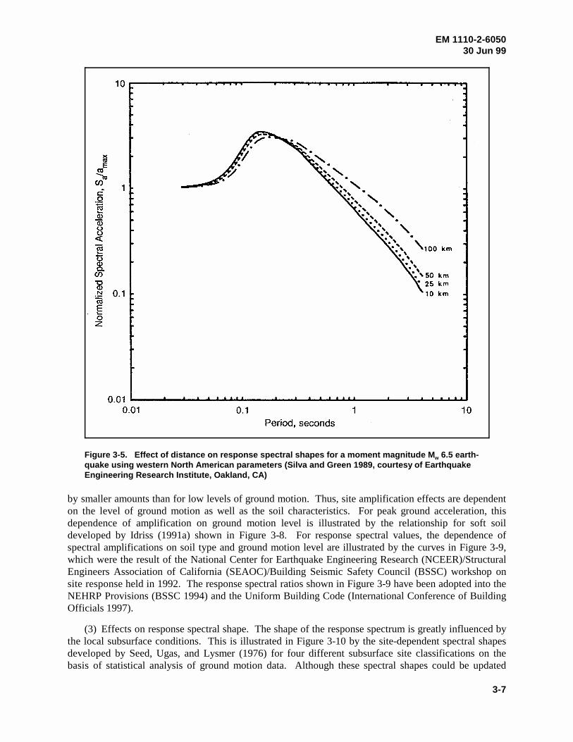
shape, in this case from the theoretically based relationships for rock of Silva and Green (1989), isillustrated in Figure 3-5. In general, within source-to-site distances of about 50 km, the effect of distanceon spectral shape is much smaller than the effect of magnitude. Similarly, although the relative durationof the strong shaking part of an accelerogram tends to increase with increasing distance (e.g., Dobry,Idriss, and Ng 1978), this effect appears to be relatively small within 50 km of an earthquake source.

(4) Special effects of near-source earthquakes. Near the earthquake source (within approximately10 to 15 km of the source), earthquake ground motions often contain a high-energy pulse of medium-to-long-period ground motion (at periods in the range of approximately 0.5 to 5 sec) that occurs when fault

EM 1110-2-605030 Jun 99

3-4

Figure 3-2. Response spectra (5 percent damped, pseudo-relative velocity)corresponding to the acceleration traces in Figure 3-1 (Anderson and Quaas (1988),courtesy of Earthquake Engineering Research Institute, Oakland, CA)

rupture propagates toward a site. It has also been found that these pulses exhibit a strong directionality,with the component of motion perpendicular (normal) to the strike of the fault being larger than thecomponent parallel to the strike (see, for example, Sadigh et al. 1993; Somerville and Graves 1993;Somerville et al. 1997). These characteristics of near-source ground motions are illustrated by theRinaldi recording obtained during the 1994 Northridge earthquake (Figure 3-6). These characteristicsshould be included in ground motion characterization for near-source earthquakes.

EM 1110-2-605030 Jun 99

3-5

Figure 3-3. Effect of magnitude M on response spectral shape of rock motions based onattenuation relationships of Sadigh et al. (1993), 30-km distance from source to site, 5 percentdamping

c. Effect of local subsurface conditions on ground motions.

(1) General. It is well established that local soil conditions have a major effect on the amplitude andresponse spectral characteristics of earthquake ground motions. It was demonstrated again by thedramatic differences in ground motions in different parts of Mexico City in the 1985 Mexico earthquake,and in different locations in the San Francisco Bay Area in the 1989 Loma Prieta earthquake.

EM 1110-2-605030 Jun 99

3-6

Figure 3-4. Variation of spectral shape with distance for rock recordings of the October 17, 1989,Loma Prieta earthquake

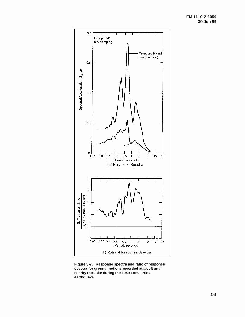
(2) Site amplification effects. Recordings obtained on different soil conditions and analytical studiesindicate that soil amplification is dependent on the type and depth of soil. Figure 3-7 illustrates theamplification of response spectra of a soft soil site recording (Treasure Island site) relative to an adjacentrock site recording (Yerba Buena site) during the Loma Prieta earthquake. The effects illustrated in Fig-ure 3-7 are qualitatively typical of those expected in soft soil for relatively low levels of ground motion(peak rock acceleration less than about 0.4 g). However, for higher levels of ground motion, higher soildamping due to nonlinear soil behavior tends to result in deamplification of high-frequency responsespectra and peak ground accelerations a while longer period components continue to be amplified butmax

EM 1110-2-605030 Jun 99

3-7

Figure 3-5. Effect of distance on response spectral shapes for a moment magnitude M 6.5 earth-w

quake using western North American parameters (Silva and Green 1989, courtesy of EarthquakeEngineering Research Institute, Oakland, CA)

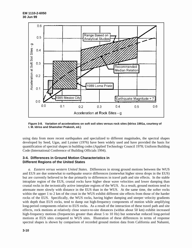
by smaller amounts than for low levels of ground motion. Thus, site amplification effects are dependenton the level of ground motion as well as the soil characteristics. For peak ground acceleration, thisdependence of amplification on ground motion level is illustrated by the relationship for soft soildeveloped by Idriss (1991a) shown in Figure 3-8. For response spectral values, the dependence ofspectral amplifications on soil type and ground motion level are illustrated by the curves in Figure 3-9,which were the result of the National Center for Earthquake Engineering Research (NCEER)/StructuralEngineers Association of California (SEAOC)/Building Seismic Safety Council (BSSC) workshop onsite response held in 1992. The response spectral ratios shown in Figure 3-9 have been adopted into theNEHRP Provisions (BSSC 1994) and the Uniform Building Code (International Conference of BuildingOfficials 1997).

(3) Effects on response spectral shape. The shape of the response spectrum is greatly influenced bythe local subsurface conditions. This is illustrated in Figure 3-10 by the site-dependent spectral shapesdeveloped by Seed, Ugas, and Lysmer (1976) for four different subsurface site classifications on thebasis of statistical analysis of ground motion data. Although these spectral shapes could be updated

EM 1110-2-605030 Jun 99

3-8

Figure 3-6. Time-histories and horizontal response spectra (5 percent damping) for the fault strike-normal(FN) and fault strike-parallel (FP) components of ground motion (V = vertical) for the Rinaldi recordingobtained 7.5 km from the fault rupture during the 1994 Northridge, California, earthquake (Somerville (1997),courtesy of Multidisciplinary Center for Earthquake Engineering Research, State University of New York atBuffalo)

EM 1110-2-605030 Jun 99

3-9

Figure 3-7. Response spectra and ratio of responsespectra for ground motions recorded at a soft andnearby rock site during the 1989 Loma Prietaearthquake

EM 1110-2-605030 Jun 99

3-10

Figure 3-8. Variation of accelerations on soft soil sites versus rock sites (Idriss 1991a, courtesy ofI. M. Idriss and Shamsher Prakesh, ed.)

using data from more recent earthquakes and specialized to different magnitudes, the spectral shapesdeveloped by Seed, Ugas, and Lysmer (1976) have been widely used and have provided the basis forquantification of spectral shapes in building codes (Applied Technology Council 1978; Uniform BuildingCode (International Conference of Building Officials 1994).

3-4. Differences in Ground Motion Characteristics inDifferent Regions of the United States

a. Eastern versus western United States. Differences in strong ground motions between the WUSand EUS are due somewhat to earthquake source differences (somewhat higher stress drops in the EUS)but are currently believed to be due primarily to differences in travel path and site effects. In the stableintraplate region of the EUS, crustal rocks have higher shear wave velocities and lower damping thancrustal rocks in the tectonically active interplate regions of the WUS. As a result, ground motions tend toattenuate more slowly with distance in the EUS than in the WUS. At the same time, the softer rockswithin the upper 1 to 2 km of the crust in the WUS exhibit different site effects from those of the harderrocks of the EUS. Specifically, the WUS rocks, having higher damping and steeper velocity gradientswith depth than EUS rocks, tend to damp out high-frequency components of motion while amplifyinglong-period components relative to EUS rocks. As a result of the interaction of these travel path and siteeffects, rock motions at relatively close source-to-site distances (within about 50 km) exhibit increasedhigh-frequency motions (frequencies greater than about 5 to 10 Hz) but somewhat reduced long-periodmotions at EUS sites compared to WUS sites. Illustration of these differences in terms of responsespectral shapes is shown by comparison of recorded ground motion data from California and Nahanni,

EM 1110-2-605030 Jun 99

3-11

Figure 3-9. Response spectral ratios relative to rock for different site classifications and ground motionlevels (BSSC 1994)

EM 1110-2-605030 Jun 99

3-12

Figure 3-10. Average acceleration spectra for different site conditions (Seed, Ugas, and Lysmer1976, courtesy of Seismological Society of America)

Canada, in Figure 3-11 (Nahanni is located in an EUS-like tectonic environment). In terms of absoluteresponse spectra, these differences are illustrated in Figures 3-12 and 3-13, where response spectra forrelatively close source-to-site distances have been calculated using the theoretical model of Silva andGreen (1989). As distance increases, the effects of travel path attenuation begin to dominate over thelocal site effects, leading to higher ground motions in the EUS over a broader frequency range.

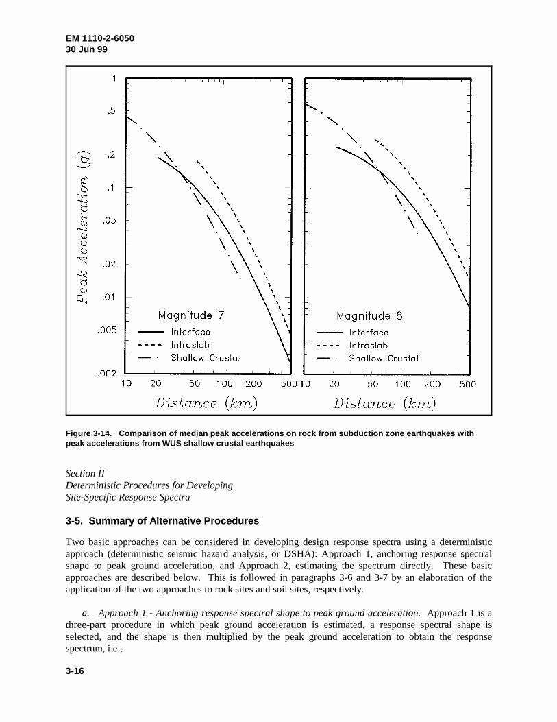
b. Subduction zone versus shallow crustal earthquakes. The collision of tectonic plates of the earthin subduction zones has caused numerous large and relatively deep earthquakes (e.g., in subduction zonesin Japan; west coast of Central and South America; coastal northwest California, Oregon, andWashington; Alaska; Puerto Rico; and many other areas). Analyses of ground motion data fromsubduction zone earthquakes indicate that the main difference between ground motions from subductionzone earthquakes and ground motions from WUS shallow crustal earthquakes is a slower rate ofattenuation for the subduction zone events. This is illustrated in Figure 3-14 in which attenuation of peakrock acceleration from shallow crustal WUS earthquakes is compared with that from subduction zoneearthquakes as determined by Youngs et al. (1993a). Attenuation curves for two types of subductionzone earthquakes are shown in Figure 3-14—interface earthquakes occurring at the interface between thesubducting tectonic plate and the overriding plate, and intraslab earthquakes occurring within the sub-ducting plate. Analyses by Youngs, Day, and Stevens (1988) and Youngs et al. (1993a) also suggest thatground motions from subduction zone earthquakes have response spectral shapes that are lower in thelong-period range than response spectral shapes for WUS shallow crustal earthquakes (Figure 3-15).

EM 1110-2-605030 Jun 99

3-13

Figure 3-11. Comparison of average 5 percent damped response spectral shapes (S /a )a max

computed from strong-motion data recorded at rock sites in Nahanni, Canada, and California forM 5.3 earthquakes (Darragh et al. 1989)w

EM 1110-2-605030 Jun 99

3-14

Figure 3-12. Comparison of response spectra for a magnitude 5 earthquake at 15 km using WUSand EUS attenuation relationships (calculated using Band-Limited-White-Noise/Random VibrationTheory (BLWN/RVT) model as formulated by Silva and Green 1989)

EM 1110-2-605030 Jun 99

3-15

Figure 3-13. Comparison of response spectra for a magnitude 6.5 earthquake at 20 km using WUSand EUS attenuation relationships (calculated using BLWN/RVT model as formulated by Silva andGreen 1989)

EM 1110-2-605030 Jun 99

3-16

Figure 3-14. Comparison of median peak accelerations on rock from subduction zone earthquakes withpeak accelerations from WUS shallow crustal earthquakes

Section IIDeterministic Procedures for DevelopingSite-Specific Response Spectra

3-5. Summary of Alternative Procedures

Two basic approaches can be considered in developing design response spectra using a deterministicapproach (deterministic seismic hazard analysis, or DSHA): Approach 1, anchoring response spectralshape to peak ground acceleration, and Approach 2, estimating the spectrum directly. These basicapproaches are described below. This is followed in paragraphs 3-6 and 3-7 by an elaboration of theapplication of the two approaches to rock sites and soil sites, respectively.

a. Approach 1 - Anchoring response spectral shape to peak ground acceleration. Approach 1 is athree-part procedure in which peak ground acceleration is estimated, a response spectral shape isselected, and the shape is then multiplied by the peak ground acceleration to obtain the responsespectrum, i.e.,

EM 1110-2-605030 Jun 99

3-17

Figure 3-15. Comparison of spectral shapes using WUS and subduction zone attenuation relationships

(1) Step 1: Estimate peak ground acceleration (PGA).

(2) Step 2: Select response spectral shape, which is the curve of spectral amplification factors,(SA /PGA), where SA is spectral acceleration at period T.T T

(3) Step 3: Obtain response spectrum as the product of the peak ground acceleration and the spectralshape, SA = PGA × (SA /PGA). This approach is often referred to as “anchoring” the spectral shape toT T

the peak ground acceleration. A variation on this approach is to estimate peak ground velocity (and, ifdesired, peak ground displacement) as well as peak ground acceleration and multiply these groundmotion parameters by the appropriate spectral amplification factors (Newmark and Hall 1978, 1982); theNewmark and Hall procedure is summarized in Appendix B.

b. Approach 2 - estimating the spectrum directly. In Approach 2 the response spectrum ordinatesare estimated directly as a single process. In general, there are three different approaches withinApproach 2 for directly estimating response spectra: using response spectral attenuation relationships;performing statistical analysis of spectra from selected ground motion records; and theoretical(numerical) modeling. These approaches are briefly outlined below.

(1) Using response spectral attenuation relationships. Attenuation relationships have beendeveloped by several investigators for response spectral values of ground motions (spectral accelerationor spectral pseudo-relative velocity) at selected periods of vibration by performing statistical regressionanalyses of ground motion data and by conducting theoretical analyses. Relationships have beendeveloped for different site conditions and tectonic environments. Specific relationships are presented inparagraph 3-6 for rock sites and paragraph 3-7 for soil sites. These relationships can be used to makeperiod-by-period estimates of response spectral values, given the design earthquake magnitude anddistance. (The zero-period spectral value is obtained from the corresponding attenuation relationship forthe peak ground acceleration, i.e., zero-period spectral acceleration (ZPA) = PGA.)

EM 1110-2-605030 Jun 99

3-18

Typically, these relationships have been developed for 5 percent damping; and ratios between spectralvalues at different damping ratios (e.g., Newmark and Hall 1978, 1982; Appendix B) are used to obtainthe corresponding spectra for other damping ratios.

(2) Performing statistical analysis of ground motion data. Spectral attenuation relationships dis-cussed above are based on all the available applicable ground motion data, and they typically cover awide range of earthquake magnitudes and distances. However, for a specific magnitude and distance, itmay be possible to obtain an improved or a comparative estimate of the response spectrum byperforming statistical analysis using a set of response spectra of ground motion records from earthquakeshaving magnitudes and distances that are close to the design magnitude and distance. The data set istypically a subset of the data used to develop attenuation relationships. The analysis may consist ofdirect, period-by-period statistical analysis of the data. However, it is also possible to “scale” or adjusteach response spectral value of each record to values for the design magnitude and distance and then dostatistical analysis of the scaled data set. The attenuation relationships for response spectral values(discussed in (1) above) are used to perform the scaling. This approach of scaling before performingstatistical analyses is recommended unless the magnitudes and distances for the data set are closelybunched around the design magnitude and distance. Appendix C illustrates the approach of statisticalanalyses of a set of scaled response spectra. A particular type of statistical analysis that has been usedfor many nuclear power plant sites in the EUS and for other sites and locations as well is termed a“random earthquake” analysis. This analysis is performed to estimate the response spectrum at a site dueto a randomly located (“floating”) earthquake within the vicinity of the site, i.e., when its location cannotbe assigned to a specific geologic structure at a specific distance from the site. After the designmagnitude of the random earthquake is selected, a statistical analysis is made of response spectra ofground motion records from earthquakes having magnitudes close to the design magnitude, recorded onsite conditions similar to those for the actual site, and recorded within a selected source-to-site distance,typically 25 km. A random earthquake analysis can also be performed using attenuation relationships.Appendix D illustrates a random earthquake analysis.

(3) Performing theoretical (numerical) ground motion modeling. The state of the art for theoretical(numerical) modeling of ground motions is being vigorously advanced and is being increasingly used forsite-specific project applications. Various methods attempt to simulate the earthquake rupture, thepropagation of seismic waves from earthquake source to site, and/or the effect of local site conditions. Anumber of methods have been developed. These methods warrant consideration as a supplementarymeans for ground motion estimation. They can be particularly useful for extrapolating to conditions thatlie outside those represented by the database of strong motion recordings. The methods vary consider-ably in degree of complexity and sophistication. One relatively simple model that has been usedincreasingly to simulate earthquake rupture and source-to-site wave propagation is the Band LimitedWhite Noise/Random Vibration Theory (BLWN/RVT) Model (Atkinson 1984; Atkinson and Boore1995; Boore 1983, 1986; Boore and Atkinson 1987; Boore and Joyner 1991; Hanks and McGuire 1981;McGuire, Toro, and Silva 1988; Silva and Green 1989). This method has been applied particularly in theEUS because of the relative scarcity of ground motion data in the EUS, and attenuation relationships forthe EUS have been developed using this model. A particular form of theoretical analysis applicable tosoil sites is “site response analysis,” or “ground response analysis” in which the objective is to assess themodifying influence of the local soil conditions on rock motions estimated for the site and, in thismanner, estimate the motions at the ground surface of the soil site. Site response analyses are discussedin paragraph 3-7 in the context of their use in estimating response spectra for soil sites.

c. Relative advantages of Approach 1 and Approach 2. Approach 2, estimating the spectrumdirectly, should be used rather than Approach 1, anchoring spectral shape to peak ground acceleration,

EM 1110-2-605030 Jun 99

3-19

because, as was outlined in Section I, spectral shapes depend on more than just the site conditions (i.e.,on tectonic environment, earthquake magnitude, and other factors), yet the readily available and widelyused spectral shapes generally incorporate only the effect of the local site conditions. Currently availableprocedures, relationships, and data enable response spectra to be estimated as a single process inApproach 2. When spectra are estimated using Approach 2, it is often useful to make comparative esti-mates using Approach 1. In paragraph 3-6 procedures and relationships for Approaches 1 and 2 fordeveloping response spectra for rock sites are discussed. A similar presentation is made in paragraph 3-7for soil sites.

3-6. Developing Site-Specific Spectra for Rock Sites

a. Using Approach 1 - Anchoring rock response spectral shape to peak rock acceleration.

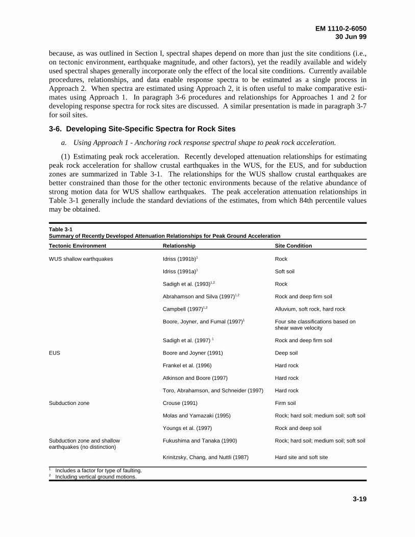
(1) Estimating peak rock acceleration. Recently developed attenuation relationships for estimatingpeak rock acceleration for shallow crustal earthquakes in the WUS, for the EUS, and for subductionzones are summarized in Table 3-1. The relationships for the WUS shallow crustal earthquakes arebetter constrained than those for the other tectonic environments because of the relative abundance ofstrong motion data for WUS shallow earthquakes. The peak acceleration attenuation relationships inTable 3-1 generally include the standard deviations of the estimates, from which 84th percentile valuesmay be obtained.

Table 3-1Summary of Recently Developed Attenuation Relationships for Peak Ground Acceleration

Tectonic Environment Relationship Site Condition

WUS shallow earthquakes Idriss (1991b) Rock1

Idriss (1991a) Soft soil1

Sadigh et al. (1993) Rock1,2

Abrahamson and Silva (1997) Rock and deep firm soil1,2

Campbell (1997) Alluvium, soft rock, hard rock1,2

Boore, Joyner, and Fumal (1997) Four site classifications based on 1

shear wave velocity

Sadigh et al. (1997) Rock and deep firm soil1

EUS Boore and Joyner (1991) Deep soil

Frankel et al. (1996) Hard rock

Atkinson and Boore (1997) Hard rock

Toro, Abrahamson, and Schneider (1997) Hard rock

Subduction zone Crouse (1991) Firm soil

Molas and Yamazaki (1995) Rock; hard soil; medium soil; soft soil

Youngs et al. (1997) Rock and deep soil

Subduction zone and shallow Fukushima and Tanaka (1990) Rock; hard soil; medium soil; soft soilearthquakes (no distinction)

Krinitzsky, Chang, and Nuttli (1987) Hard site and soft site

Includes a factor for type of faulting.1

Including vertical ground motions.2

EM 1110-2-605030 Jun 99

3-20

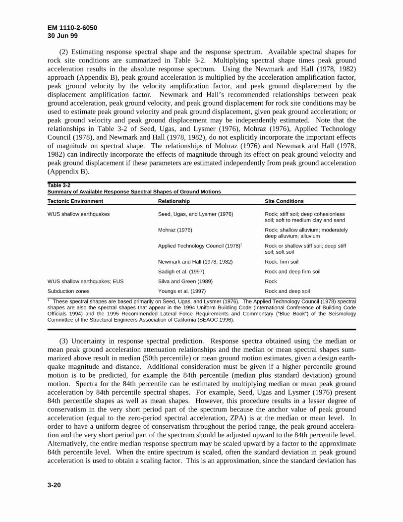
(2) Estimating response spectral shape and the response spectrum. Available spectral shapes forrock site conditions are summarized in Table 3-2. Multiplying spectral shape times peak groundacceleration results in the absolute response spectrum. Using the Newmark and Hall (1978, 1982)approach (Appendix B), peak ground acceleration is multiplied by the acceleration amplification factor,peak ground velocity by the velocity amplification factor, and peak ground displacement by thedisplacement amplification factor. Newmark and Hall’s recommended relationships between peakground acceleration, peak ground velocity, and peak ground displacement for rock site conditions may beused to estimate peak ground velocity and peak ground displacement, given peak ground acceleration; orpeak ground velocity and peak ground displacement may be independently estimated. Note that therelationships in Table 3-2 of Seed, Ugas, and Lysmer (1976), Mohraz (1976), Applied TechnologyCouncil (1978), and Newmark and Hall (1978, 1982), do not explicitly incorporate the important effectsof magnitude on spectral shape. The relationships of Mohraz (1976) and Newmark and Hall (1978,1982) can indirectly incorporate the effects of magnitude through its effect on peak ground velocity andpeak ground displacement if these parameters are estimated independently from peak ground acceleration(Appendix B).

Table 3-2Summary of Available Response Spectral Shapes of Ground Motions

Tectonic Environment Relationship Site Conditions

WUS shallow earthquakes Seed, Ugas, and Lysmer (1976) Rock; stiff soil; deep cohesionlesssoil; soft to medium clay and sand

Mohraz (1976) Rock; shallow alluvium; moderatelydeep alluvium; alluvium

Applied Technology Council (1978) Rock or shallow stiff soil; deep stiff1

soil; soft soil

Newmark and Hall (1978, 1982) Rock; firm soil

Sadigh et al. (1997) Rock and deep firm soil

WUS shallow earthquakes; EUS Silva and Green (1989) Rock

Subduction zones Youngs et al. (1997) Rock and deep soil

These spectral shapes are based primarily on Seed, Ugas, and Lysmer (1976). The Applied Technology Council (1978) spectral1

shapes are also the spectral shapes that appear in the 1994 Uniform Building Code (International Conference of Building CodeOfficials 1994) and the 1995 Recommended Lateral Force Requirements and Commentary (“Blue Book”) of the SeismologyCommittee of the Structural Engineers Association of California (SEAOC 1996).

(3) Uncertainty in response spectral prediction. Response spectra obtained using the median ormean peak ground acceleration attenuation relationships and the median or mean spectral shapes sum-marized above result in median (50th percentile) or mean ground motion estimates, given a design earth-quake magnitude and distance. Additional consideration must be given if a higher percentile groundmotion is to be predicted, for example the 84th percentile (median plus standard deviation) groundmotion. Spectra for the 84th percentile can be estimated by multiplying median or mean peak groundacceleration by 84th percentile spectral shapes. For example, Seed, Ugas and Lysmer (1976) present84th percentile shapes as well as mean shapes. However, this procedure results in a lesser degree ofconservatism in the very short period part of the spectrum because the anchor value of peak groundacceleration (equal to the zero-period spectral acceleration, ZPA) is at the median or mean level. Inorder to have a uniform degree of conservatism throughout the period range, the peak ground accelera-tion and the very short period part of the spectrum should be adjusted upward to the 84th percentile level.Alternatively, the entire median response spectrum may be scaled upward by a factor to the approximate84th percentile level. When the entire spectrum is scaled, often the standard deviation in peak groundacceleration is used to obtain a scaling factor. This is an approximation, since the standard deviation has

EM 1110-2-605030 Jun 99

3-21

been found to vary with period of vibration. (The period dependence can be directly accounted for whenusing Approach 2.) The 84th percentile amplification factors of the Newmark and Hall (1978, 1982)approach can be applied to median estimates of peak ground acceleration, velocity, and displacement toobtain 84th percentile spectral values (Appendix B, Table B-1). Again, a separate adjustment should beapplied to raise the peak ground acceleration and very short period part of the spectrum to the 84thpercentile level.

(4) Estimating vertical ground motion response spectra. Ratios of vertical to horizontal responsespectral amplitudes can be used to estimate vertical response spectra, given an estimate of horizontalresponse spectra. Recent studies (e.g., Silva 1997) indicate that vertical-to-horizontal response spectralratios are a function of period of vibration, earthquake source to site distance, earthquake magnitude,tectonic environment (WUS and EUS), and subsurface conditions (soil and rock). Figure 3-16 provides aguideline for ratios of vertical to horizontal spectral values on rock sites that is generally conservative forearthquake magnitudes equal to or less than about 6.5. However, if a facility is sensitive to short-period(less than 0.3 sec) vertical motions, and is located within 10 km of the earthquake source or the magni-tude exceeds 6.5, further evaluation of vertical response spectra on rock is recommended because verticalresponse spectra can significantly exceed horizontal response spectra for these conditions.

b. Using Approach 2 - Estimating the rock response spectrum directly.

(1) General. The three approaches discussed in paragraph 3-5b can be used: using response spectralattenuation relationships, performing statistical analyses of ground motion response spectra, andtheoretical (numerical) modeling. The following paragraphs refer to particular relationships or methods.

(2) Using response spectral attenuation relationships. Recently developed attenuation relationshipsthat can be used to predict horizontal rock response spectral values for WUS shallow crustal earthquakes,for EUS earthquakes, and for subduction zone earthquakes are summarized in Table 3-3. The spectralacceleration attenuation relationships summarized in Table 3-3 generally include the standard deviationsof the estimates, from which 84th percentile values may be obtained. As illustrated in Figures 3-12 and3-13, EUS attenuation models characteristically estimate much higher spectral response in the short-period range (less than 0.1 to 0.2 sec) than estimated by relationships for the WUS. As discussed inparagraph 3-4a the higher short-period response is attributed to the hardness of the rock in the EUS.Such short-period (high-frequency) motions may or may not be significant to the response andperformance of hydraulic structures. The assessment of the significance of such motions should be madeby the principal design engineer in collaboration with the seismic structural analyst and the materialsengineer.

(3) Using statistical analyses of response spectra. Abundant strong motion data are available to per-mit statistical analyses of data sets for many design earthquake scenarios for WUS shallow crustal earth-quakes. As noted in paragraph 3-5b(2), statistical “random earthquake” analyses have been made atmany EUS sites because, in general, discrete faults have not been identified in the EUS. Yet it wasdesired to model the possibility of an earthquake (usually of moderate magnitude, in the range of magni-tude 5 to 6) occurring near the site. Many of these analyses have been carried out using WUS groundmotion data because only a few records from moderate magnitude earthquakes are available in the EUS.Such analyses may be reasonable for estimating longer period rock motions but would apparently under-estimate shorter period (less than 0.1 to 0.3 sec) ground motions at hard rock sites. In this case, anadjustment should be made for the short-period response spectral values, if these short-period motionsare of significance to the structure under consideration. The adjustment can be made by comparing

EM 1110-2-605030 Jun 99

3-22

Figure 3-16. Simplified relationships between vertical and horizontal response spectra as a function ofdistance R

EM 1110-2-605030 Jun 99

3-23

Table 3-3Summary of Recently Developed Attenuation Relationships for Response Spectral Values of Ground Motions

Tectonic Environment Relationship Site Conditions

WUS shallow earthquakes Idriss (1991b) Rock1

Sadigh et al. (1993) Rock1,2

Abrahamson and Silva (1997) Rock and deep firm soil1,2

Campbell (1997) Alluvium, soft rock, hard rock1,2

Boore, Joyner, and Fumal (1997) Four site classifications based on1

shear wave velocity

Sadigh et al. (1997) Rock and deep firm soil1

EUS Boore and Joyner (1991) Deep soil

Frankel et al. (1996) Hard rock

Atkinson and Boore (1997) Hard rock

Toro, Abrahamson, and Schneider (1997) Hard rock

Subduction zone Crouse (1991) Firm soil

Youngs et al. (1997) Rock and deep soil

Includes a factor for type of faulting.1

Including vertical ground motions.2

response spectrum amplitudes predicted by EUS and WUS attenuation relationships for rock (Table 3-3).As illustrated in Appendix D, a random earthquake analysis can also be carried out using attenuationrelationships. Thus this analysis can be performed using the EUS spectral attenuation relationships thatpredict higher short-period motions at hard rock sites.

(4) Using theoretical (numerical) modeling techniques. The techniques discussed in para-graph 3-5b(3) can be used. These techniques attempt to simulate the earthquake rupture and the propaga-tion of seismic waves from the earthquake source to the site.

(5) Estimating vertical ground motion response spectra. The available recently developed attenua-tion relationships for response spectral values of vertical rock motions are summarized in Table 3-3.These relationships can be used directly to estimate vertical rock response spectra. The vertical to hori-zontal spectral ratios discussed in paragraph 3-6a(4) and shown in Figure 3-16 can be used as a guide inestimating vertical response spectra, given an estimate of the horizontal spectra.

c. Developing acceleration time-histories of rock motions consistent with the design responsespectrum.

(1) General. When acceleration time-histories of ground motions are required for the dynamicanalysis of a structure, they should be developed to be consistent with the design response spectrum overthe period range of significance for the structure, as well as have an appropriate strong motion durationfor the particular design earthquake. Two general approaches to developing acceleration time-historiesare selecting a suite of recorded motions and synthetically developing or modifying one or more motions.

EM 1110-2-605030 Jun 99

3-24

These approaches are discussed below. For either approach, when near-source earthquake groundmotions are modeled, it may be desirable that an acceleration time-history include a strong intermediate-to long-period pulse to model this particular characteristic of ground motion often observed in the nearfield (paragraph 3-3b(4) and Figure 3-6).

(2) Selecting recorded motions. Every earthquake produces a unique set of acceleration time-histories having characteristics that depend on the earthquake magnitude and other source characteristics,distance, attenuation and other travel path characteristics, and local site conditions. The response spec-trum of any individual ground motion accelerogram has peaks and valleys that occur at different periodsof vibration. Thus, the response spectrum of any single accelerogram is unlikely to match the developedsmooth design response spectrum. Typically, when recorded motions are selected, it is necessary tochoose a suite of time-histories (typically at least four) such that, in aggregate, valleys of individualspectra that fall below the design curve are covered by peaks of other spectra and (preferably) theexceedance of the design spectrum by individual spectral peaks is not excessive. For nonlinear analyses,it may be desirable to have additional time-histories because of the importance of pulse sequencing tononlinear response (see also comments in (3) below). In the approach of selecting recorded motions,simple scaling of individual accelerograms by a constant factor is done to improve the spectral fit, but thewave form and the relative spectral content of the accelerograms are not modified. The advantage ofselecting recorded motions is that each accelerogram is an actual recording, and thus the structure isanalyzed for natural motions that are presumably most representative of what the structure could expe-rience. The approach has the following disadvantages: multiple dynamic analyses are needed for thesuite of accelerograms selected; although a suite of accelerograms is selected, there will typically besubstantial exceedances of the smooth design spectrum by individual spectrum peaks; and although areasonably good spectral fit may be achieved for one horizontal component, when the same simplescaling factors are applied to the other horizontal components and the vertical components for the recordsselected, the spectral fit is usually not as good for the other components.

(3) Synthetically developing or modifying motions. A number of techniques and computer programshave been developed either to completely synthesize an accelerogram or modify a recorded accelerogramso that the response spectrum of the resultant accelerogram closely fits or matches the design spectrum.It is preferred to use techniques that modify a recorded accelerogram rather than completely synthesize amotion since the recorded motion will have time-domain characteristics representative of actual groundmotions. Two techniques that have been found to do a good job of spectrally modifying recordedmotions are the frequency-domain RASCAL computer code developed for the Corps of Engineers bySilva and Lee (1987) and the time-domain technique developed by Lilhanand and Tseng (1988). Thesetechniques preserve the basic time-domain character of the accelerogram yet provide an excellent matchto a smooth spectrum. An example of the spectral matching technique is given in Figures 3-17 and 3-18.The RASCAL computer code was used in this case. Figure 3-17 illustrates the initial (recorded)acceleration, velocity, and displacement time-histories and the time-histories after the spectral matchingprocess. Figure 3-18 illustrates the initial (recorded) acceleration response spectra, the smooth designresponse spectrum, and the response spectrum of the acceleration time-history after the spectral matchingprocess. Figure 3-18 illustrates the very close spectral match that was achieved, while Figure 3-17illustrates that the modified time-histories preserve the basic time-domain character of the originalrecord. Synthetic techniques for developing time-histories have the following advantages: a good fit tothe design spectrum can be achieved with a single accelerogram; the natural appearance and strongmotion duration can be maintained in the accelerograms; and three component motions (two horizontaland one vertical) each providing a good spectral match can be developed, and these can be madestatistically independent if desired; and the process is relatively efficient.

EM 1110-2-605030 Jun 99

3-25

Figure 3-17. Example of original time-histories and time-histories after a spectral matching process

EM 1110-2-605030 Jun 99

3-26

Figure 3-18. Example of response spectrum of time-history matched to a designresponse spectrum and spectrum of original time-history

The disadvantage is that the motions are not “real” motions, which would not exhibit smoothdesign spectra. Also “real” motions may contain less energy than synthetic spectrum-matched motionsof similar amplitude. Although a good fit to a design spectrum can be attained with a single accelero-gram, it may be desirable in some cases to fit the spectrum using more than one accelerogram. Fornonlin ear analysis applications, it is particularly desirable to have multiple accelerograms becausedifferent accelerograms may have different pulse sequencing characteristics of importance to nonlinearresponse yet have essentially identically response spectra. Numerical ground motion modeling methodscan also be used to produce synthetic accelerograms. Such motions have the character of recordedmotions since the modeling procedures are intended to simulate the earthquake rupture and wavepropagation process.

EM 1110-2-605030 Jun 99

3-27

3-7. Developing Site-Specific Spectra for Soil Sites

As is the case for developing site-specific rock spectra, either the approach of anchoring spectral shapesto a peak ground acceleration (Approach 1) or the approach of directly estimating the spectra(Approach 2) can be used for soil sites. The implementation of these approaches is outlined below.

a. Approach 1 - Anchoring the response spectral shape to the peak ground acceleration.

(1) Estimating peak ground acceleration. Table 3-1 summarizes recently developed attenuation rela-tionships for estimating peak ground acceleration. For WUS shallow crustal faulting earthquakes,several recent attenuation relationships are available to estimate top-of-soil peak ground accelerations forfirm soil conditions, and Idriss (1991a) has developed a peak acceleration attenuation relationship forsoft soil sites. Combining the BLWN/RVT method for rock motion estimation with a site responseanalysis for a deep soil column, Boore and Joyner (1991) developed a peak ground accelerationattenuation relationship for deep soil sites in the EUS. For subduction zone earthquakes, attenuationrelationships have been developed for firm soil conditions and in some cases for soft soil conditions(Table 3-1). As is the case for rock attenuation relationships, the soil attenuation relationships are betterconstrained by data for WUS shallow crustal earthquakes than for EUS or subduction zone earthquakes.

(2) Estimating response spectral shape and the response spectrum. Spectral shapes that have beendeveloped for soil sites for WUS shallow crustal earthquakes and for subduction zone earthquakes on thebasis of statistical analyses of ground motion data are summarized in Table 3-2. Spectral shapes have notbeen developed for soil sites for EUS earthquakes. Using the Newmark and Hall (1978, 1982) approach(Appendix B), the effect of soil is accounted for by estimating values of peak ground velocity and peakground displacement directly, or by using Newmark and Hall’s relationships between peak groundacceleration, peak ground velocity, and peak ground displacement for firm soil to estimate peak groundvelocity and peak ground displacement, given peak ground acceleration. Peak ground acceleration,velocity, and displacement then are multiplied by Newmark and Hall’s amplification factors to obtain theabsolute response spectrum.

(3) Uncertainty in response spectra predictions. The comments made in paragraph 3-6a(3) regardingestimating 84th percentile response spectra for rock also apply to response spectra for soil.

(4) Estimating vertical ground motion response spectra. Recent studies (e.g., Silva 1997) indicatethat vertical-to-horizontal ratios of response spectra of ground motions are higher on soil than on rock forshort periods of vibration. Figure 3-16 provides a guideline for ratios of vertical-to-horizontal spectralratios on firm soil sites that is generally conservative. However, if a facility is sensitive to short-period(less than 0.3 sec) vertical motions, and is located within 25 km of the earthquake source or themagnitude exceeds 6.5, further evaluation of vertical response spectra on soil is recommended becausevertical response spectra can significantly exceed horizontal response spectra for these conditions.

b. Using Approach 2 - Estimating the soil response spectrum directly.

(1) General. The three approaches discussed in paragraph 3-5b can be used for soil sites. Theseapproaches are using response spectral attenuation relationships, performing statistical analysis of groundmotion response spectra, and theoretical (numerical) modeling.

(2) Using response spectral attenuation relationships. Recently developed response spectralattenuation relationships for soil are summarized in Table 3-3. The spectral attenuation relationships in

EM 1110-2-605030 Jun 99

3-28

Table 3-3 generally include the standard deviations of the estimates, from which 84th percentile valuesmay be obtained.

(3) Using statistical analyses of response spectra. Abundant ground motion data for firm soil sites inthe WUS are available to permit statistical analyses of data sets for many design earthquakes. Althoughsuch data are not available for EUS earthquakes, the WUS data can be used, recognizing that the analysesmay underestimate short-period (less than 0.1 to 0.3 sec) response spectra. (Refer to discussion for rocksites in paragraph 3-6b(3).) The degree of underestimation should be less at soil sites than at rock sitesbecause soils will tend to damp out the short-period motions.

(4) Using theoretical (numerical) modeling techniques. The techniques discussed in para-graph 3-5b(3) can be used to simulate the earthquake rupture and propagation of seismic waves from theearthquake source to the site. In addition, site response analyses may be carried out to estimate top-of-soil response spectra, given a response spectrum in rock. With this approach, rock motions, includingresponse spectra, are first defined for the site (using procedures and relationships described in para-graph 3-6). The soil profile between the ground surface and the underlying rock is modeled. The rockmotions are assigned to a hypothetical rock outcrop at the site rather than to the rock at depth beneath thesoil column. This is because rock motion recordings are obtained at the ground surface rather than atdepth, and unless the rock is rigid, the rock motion beneath the soil column will differ somewhat from therock outcrop motion. Then, using nonlinear or equivalent linear soil response analytical methods, rockmotions are propagated through the soils column and top-of-soil motions are estimated. The siteresponse analysis process is schematically illustrated in Figure 3-19. This figure illustrates thecommonly used one-dimensional site response analysis method applicable where the soil stratigraphy isrelatively uniform and flat-lying and the ground surface topography is relatively level. Two-dimensionalsite response analysis methods are available for situations where these conditions are not sufficientlymet. Just as in other types of theoretical modeling and numerical analyses, results of site responseanalyses are sensitive to the details of the analytical procedures, modeling of the process, and inputs tothe analysis. Broad guidelines for conducting these analyses are listed below:

(a) More than one input rock acceleration time-history should be used, and the selected motionsshould be reasonably representative of the rock motions in terms of spectra and duration.

(b) Parametric analyses for variations in the dynamic soil properties should be made to examine thesensitivity of the response to uncertainties in the soil properties. This is particularly important when soilproperties are based on generalized correlations rather than on a program of field shear wave velocitymeasurements.

(c) It is useful to compute ratios of response spectra of top-of-soil motion to input rock motion foreach analysis that is carried out. The ratios are much less sensitive to the actual input motion than is theabsolute top-of-soil motion. The spectral ratios can then be examined and smoothed and multiplied bythe rock smooth spectrum to obtain a top-of-soil spectrum, which can be further smoothed.

An illustration of a site response analysis is presented in Appendix E. Articles by Seed and Sun (1989),Chang et al. (1990), and Ahmad, Gazetas, and Desai (1991) provide useful background information onsite response analysis methodologies. Site response analyses are needed relatively more for soft soil sitesthan for firm soil sites because the site response effects are greater for soft soils and because groundmotion data and empirically based ground motion relationships are relatively scarce for soft soil sites.

EM 1110-2-605030 Jun 99

3-29

Figure 3-19. Schematic of one-dimensional siteresponse analysis

(5) Estimating vertical ground motion response spectra. The available recently developedattenuation relationships for response spectral accelerations of vertical firm-soil site motions aresummarized in Table 3-3. These relationships can be used directly to estimate vertical response spectraon firm soils sites. The vertical to horizontal response spectral ratios discussed in paragraph 3-7a(4) andshown in Figure 3-16 can be used as a guide in estimating vertical response spectra, given an estimate ofhorizontal response spectra.

c. Developing acceleration time-histories of soil motions consistent with design response spectrum.The two alternatives for developing acceleration time-histories for rock motions that were discussed in

pE(z) 1 e(�z # t)

EM 1110-2-605030 Jun 99

3-30

paragraph 3-6c, namely, selecting recorded motions and synthetically developing or modifying motions,can also be used to develop time-histories for top-of-soil motions. In the case where site responseanalyses are carried out to define top-of-soil motions, there is a third alternative, which is to obtain thetime-histories directly from the site response analyses.

Section IIIProbabilistic Approach for Developing Site-Specific Response Spectra

3-8. Overview of Probabilistic Seismic Hazard Analysis (PSHA) Methodology

a. General. PSHA takes the elements of a deterministic assessment of earthquake ground shakinghazard—identification of seismic sources; specification of limiting earthquake sizes; assessment ofground motions as a function of earthquake magnitude; source-to-site distance; and site conditions—andadds an assessment of the likelihood that ground shaking will occur during a specified time period. Fig-ure 3-20 shows a typical result of PSHA, termed a hazard curve, that relates the level of ground shakingto the annual frequency of exceedance of that level. The ground motion parameter for the example inFigure 3-20 is peak ground acceleration. PSHA may be conducted for other ground motion parameters,such as peak ground velocity or response spectral values for specific periods of vibration and dampingratios. If a PSHA is carried out for response spectral values at a number of periods of vibration, thenresponse spectra having selected probabilities of exceedance (i.e., “equal hazard” response spectra) maybe constructed, as will be discussed later.

b. Elements of a PSHA. Evaluation of the frequency or probability of exceedance of groundmotions at a site is a function of earthquake source definition (distance of the sources from the site,source geometries, and frequencies of occurrence (recurrence) of earthquakes of different magnitudes oneach source), and ground motion attenuation (amplitudes of ground motion as a function of earthquakemagnitude and distance). These basic inputs to a PSHA are then combined in a probabilistic model toobtain hazard curves and (if desired) equal-hazard response spectra as discussed above. The basicelements of a PSHA are illustrated in Figure 3-21 for peak ground acceleration and in Figure 3-22 forequal hazard response spectra.

c. Formulation of PSHA methodology.

(1) Formulation. The methodology used to conduct PSHA was initially developed by Cornell(1968). Current practice is described in several publications, such as National Research Council (1988)and Earthquake Engineering Research Institute Committee on Seismic Risk (1989). Using a Poissonprobability model (paragraph 3-9d), the probability of exceedance p (z) of a ground motion level z in anE

exposure time or design time period t at a site is related to the annual frequency of ground motionexceedance at the site, � , by:z

(3-1)

A PSHA is carried out to obtain � , and p (z) can then be obtained using Equation 3-1. The return periodz E

(RP) for ground motion exceedance at a site is equal to the reciprocal of � . The results of a PSHA are,z

in practice, expressed in terms of one or more of the parameters, p (z), � , and RP. Using Equation 3-1,E z

the interrelationship between these fundamental parameters is illustrated in graphical form in Figure 3-23and in tabular form in Table 3-4. Note that when (� •t) is small (approximately � 0.1), p (z) isz E

approximately equal to � •t. For larger values of � •t, p (z) is less than (� •t). The basic formulation forz z E z

� is:z

vz�N�M� (mi) •�

RP (Rrj |mi) • P (Z > z mi rj)

n

�N

EM 1110-2-605030 Jun 99

3-31

Figure 3-20. Example seismic hazard curve showing relationship between peak groundacceleration and probability (annual frequency) of exceedance

(3-2)

where

= summation over all (N) seismic sources

�(m ) = the annual frequency of occurrence of earthquakes of magnitude m (above a certaini i

minimum size of engineering significance) on seismic source n

EM 1110-2-605030 Jun 99

3-32

Figure 3-21. Development of response spectrum based on a fixed spectrum shape and aprobabilistic seismic hazard analysis for peak ground acceleration

P (R=r m ) = the probability of an earthquake of magnitude m on source n occurring at a certainj i i

distance r from the sitej

P (Z>z m ,r ) = the probability that ground motion level z will be exceeded, given an earthquake ofi j

magnitude m on source n at distance r from the sitei j

EM 1110-2-605030 Jun 99

3-33

Figure 3-22. Development of equal-hazard response spectrum from probabilistic seismic hazardanalysis for response spectral values

Thus, for a given source, the annual frequency or rate of exceeding a certain ground motion level at thesite is obtained by summing over all magnitudes and source-to-site distances for that source. Then, thetotal rate of ground motion exceedance at the site � is obtained by adding the rates for all the sources.z

The components of Equation 3-2 are discussed in (2), (3), and (4) below. A simplified example of aPSHA illustrating the calculation process using Equation 3-2 is presented in Appendix G (Example G-1).

EM 1110-2-605030 Jun 99

3-34

Figure 3-23. Relationship between annual frequency of exceedance/return period and probability ofexceedance for different design time periods

(2) Rate of occurrence of earthquakes. The rate of occurrence of earthquakes �(m ) is obtainedi

based on earthquake recurrence assessments. Typical earthquake recurrence curves for earthquakesources are illustrated in the upper part of Figure 3-24. As shown, recurrence curves express the rate ofoccurrence of earthquakes equal to or greater than a certain magnitude. �(m ) is obtained by discretizingi

the recurrence curves into narrow magnitude intervals as illustrated in the lower part of Figure 3-24. Thetwo different types of magnitude distributions shown in Figure 3-24, exponential and characteristic, arediscussed in paragraph 3-9(d).

EM 1110-2-605030 Jun 99

3-35

Table 3-4Relationship Between Return Period and Probability of Exceedance for Different Time Periods

Return Period, Years, for Different Design Time Periods t

Probability of t = t = t = t = t = t =Exceedance, % 10 years 20 years 30 years 40 years 50 years 100 years

1 995 1,990 2,985 3,980 4,975 9,950

2 495 990 1,485 1,980 2,475 4,950

5 195 390 585 780 975 1,950

10 95 190 285 380 475 950

20 45 90 135 180 225 450

30 28 56 84 112 140 280

40 20 39 59 78 98 195

50 14 29 43 58 72 145

60 11 22 33 44 55 110

70 8.3 17 25 33 42 83

80 6.2 12 19 25 31 62

90 4.3 8.7 13 17 22 43

95 3.3 6.7 10 13 17 33

99 2.2 4.3 6.5 8.7 11 22

99.5 1.9 3.8 5.7 7.5 9.4 19

(3) Distance probability distribution. The distance probability distribution, P(R=r m ), depends onj i

the geometry of earthquake sources and their distance from the site; an assumption is usually made thatearthquakes occur with equal likelihood on different parts of a source. The function P(R=r m ) alsoj i

should incorporate the magnitude-dependence of earthquake rupture size; larger magnitude earthquakeshave larger rupture areas, and thus have higher probability of releasing energy closer to a site thansmaller magnitude earthquakes on the same source. An example of probability distributions for theclosest distance to an earthquake source is shown in Figure 3-25. In this particular example, the source(fault) is characterized as a line source, and the probability distributions are based on the formulationspresented by Der Kiureghian and Ang (1977). Figure 3-25a illustrates the probability distributions for afault rupture length of 5 km; Figure 3-25b illustrates the probability distributions for a fault rupturelength of 25 km. The longer rupture length corresponds to a larger magnitude. The figure shows thedistributions for both the probability of the closest distance to the fault rupture R being less than a certainvalue P(R<r m ), and the probability of earthquakes occurring at a certain distance (P(R=r m ), whichj i j i

is obtained by discretizing the curves for P(R<r m ). The higher probability for earthquakes to occur atj i

closer distances for longer rupture lengths (larger magnitudes) can be noted by comparing Figure 3-25bwith 3-25a. It can also be observed in Figure 3-25 that there is zero probability of earthquake occurrenceeither closer than the closest distance to the earthquake source (10 km in the example) or farther than theclosest distance to the rupture placed at the farthest end of the fault (farther than a distance ofapproximately 61 km [10 + (65 - 5) ] for a 5-km rupture and a distance of approximately 41 km2 2 ½

[10 + (65 - 25) ] in the case of the 25-km rupture length). The probability abruptly changes at a closest2 2 ½

distance equal to the distance defined by placing the fault rupture at the nearest end of the fault (distanceof approximately 32 km [10 + (35 - 5) ] for a 5-km rupture and a distance of approximately 14 km2 2 ½

[10 + (35 - 25) ] for a 25-km rupture). Note that the distance to the earthquake rupture must be2 2 ½

EM 1110-2-605030 Jun 99

3-36

Figure 3-24. Typical earthquake recurrence curves and discretized occurrence rates

expressed in terms of the same definition of distance as used in the ground motion attenuation rela-tionships. Typically, some form of closest distance to rupture definition is used for attenuation relation-ships (variations in this definition include closest distance to rupture, closest distance to rupture of theseismogenic zone, closest horizontal distance to surface projection of rupture, etc.).

EM 1110-2-605030 Jun 99

3-37

Figure 3-25. Illustration of distance probability distribution

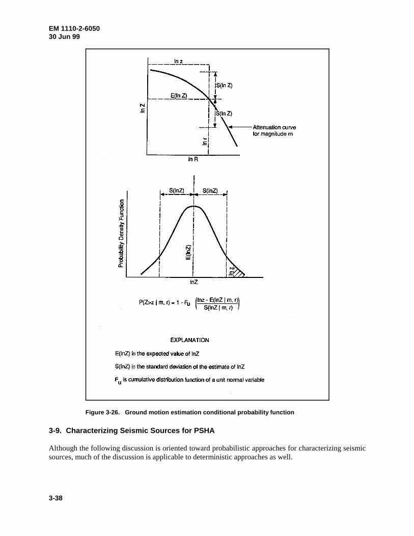
(4) Conditional probability of ground motion exceedance. The conditional probability of exceedinga ground motion level for a certain earthquake magnitude and distance P(Z>z m,r) is determined fromthe ground motion attenuation relationships selected for the site. (Available relationships are discussedin Section II.) These relationships incorporate the uncertainty in ground motion estimation given m and r(see Figures 3-21 and 3-22). The function P(Z>z m,r) is usually evaluated assuming that ground motionvalues are log normally distributed about the median value; the calculation of this function is illustratedin Figure 3-26.

EM 1110-2-605030 Jun 99

3-38

Figure 3-26. Ground motion estimation conditional probability function

3-9. Characterizing Seismic Sources for PSHA

Although the following discussion is oriented toward probabilistic approaches for characterizing seismicsources, much of the discussion is applicable to deterministic approaches as well.

EM 1110-2-605030 Jun 99

3-39

a. Source identification.

(1) Seismic source. A seismic source represents a region of the earth's crust where thecharacteristics of earthquake activity are recognized to be different from those of the adjacent crust.Seismic sources are identified on the basis of geological, seismological, and geophysical data. An under-standing of the regional tectonics, local Quaternary geologic history, and seismicity of an area leads tothe identification of seismic sources. The development of tectonic models for crustal deformation andthe assessment of the tectonic role of individual geologic structures are useful for both identifyingpotential sources and assessing their characteristics. Geologic studies can be used to assess the location,timing, and style of crustal deformation. The association of geologic structures with historic or instru-mental seismicity may clarify their role within the present tectonic stress regime. Characteristics ofseismicity, including epicenter locations, focal depths, and source mechanisms, also aid in identifyingpotential sources.

(2) Faults. Because earthquakes occur as a result of differential slip on faults, modeling of seismicsources as individual faults is the most physically realistic model for seismic hazard analysis. Underfavorable conditions, individual faults can be identified and treated as distinct seismic sources. Activefaults are usually identified on the basis of geomorphic expression and stratigraphic displacements butcan also be identified by lineations of seismicity, by geophysical measurements, or by inference fromdetailed investigations of related geologic structures, such as active folding or crustal plate subduction.A fault model for individual sources allows the use of geologic data on fault behavior, as well asseismicity data, to characterize earthquake activity.

(3) Seismic source zones. In areas with low rates of crustal deformation away from plate margins,such as the EUS, seismic sources are often defined as seismic source zones. Seismic source zones areused to model the occurrence of seismicity in areas where specific faults cannot be identified and wherethe observed seismicity exhibits a diffuse pattern not clearly associated with individual faults. Theseconditions are typical of areas with lower rates of crustal deformation, such as regions away from platemargins (e.g., EUS). Seismic source zones can be defined based either on historical seismicity patternsor geology and tectonics. When defined based on historical seismicity patterns, a large region can besubdivided into small regular areas that are treated as individual source zones (Electric Power ResearchInstitute (EPRI) 1987; U.S. Geological Survey (USGS) 1996). With this approach, it is assumed that thespatial variation in the occurrence rate of future earthquakes is similar to the historical pattern ofseismicity. Due to the relatively short historical period and low rates of seismicity, the seismicitypatterns are usually determined by small earthquakes. It is not clear whether this pattern reflects thelikelihood of future earthquakes of engineering significance (generally taken to be earthquakes ofmagnitude approximately equal to or greater than 5). The alternative approach is to define areas thoughtto have homogeneous earthquake potential characteristics (in terms of rate of earthquake occurrence andmaximum earthquake size) on the basis of the geology and tectonics of the region. For example, recentevidence from studies of global earthquakes in stable continental regions such as the EUS has shown thatmost larger earthquakes occur through reactivation of faults in geologically ancient rift zones (Johnstonet al. 1994). Where available, paleoseismological data (e.g., spatial and temporal distribution ofliquefaction features) should be used to identify source regions for large-magnitude earthquakes.Because of uncertainty regarding the most appropriate model for earthquake occurrence, both seismicity-based and geologically based seismic source zones should be included in a probabilistic analysis.

b. Source geometry.

(1) General. Description of the geometry of a seismic source is necessary to evaluate the distancesfrom the site at which future earthquakes could occur. In addition, source geometry can place physicalconstraints on the maximum size earthquake that can occur on a source.

EM 1110-2-605030 Jun 99

3-40

(2) Faults. Seismic sources defined as faults are modeled in a PSHA as segmented linear or planarfeatures. Earthquake ruptures on fault sources are modeled as rupture lengths or rupture areas, with thesize of rupture defined on the basis of empirical relationships between earthquake magnitude and rupturesize (Wyss 1979; Wells and Coppersmith 1993).

(3) Seismic source zones. For seismic sources defined as geologic structures suspected to containfaults, the distribution of earthquakes can be modeled as rupture surfaces occurring on multiple faultplanes distributed throughout the source volume if the general trend of such planes is known or can beinferred. Alternatively, earthquake locations can be modeled as random point sources within the sourcevolume if the orientation of potential fault planes is unknown. The spatial distribution of seismicitywithin large areal sources can be modeled similarly.

c. Maximum earthquake magnitude.

(1) Faults. The limiting size earthquake that can occur on each seismic source is an importantparameter, especially in evaluating seismic hazard at low probability levels. The maximum magnitudecan most easily be estimated when the seismic source is defined on the basis of an identifiable fault. Forfaults, the maximum earthquake magnitude is related to fault geometry and fault behavior through anassessment of the maximum dimensions of a single rupture. Evaluation of fault segmentation can play akey role in identifying portions of a fault zone likely to represent the largest size of a single rupture(Schwartz and Coppersmith 1986; Schwartz 1988). The maximum magnitude is related to the maximumrupture size through empirical relationships (Slemmons 1982; Bonilla, Mark, and Lienkaemper 1984;Wells and Coppersmith 1994). Because these relationships are subject to uncertainty, the use of anumber of magnitude estimation techniques can result in more reliable estimates of maximum magnitudethan the application of a single relationship.

(2) Seismic source zones. The assessment of maximum magnitude is more difficult when seismicsources are defined on the basis of large-scale tectonic features or crustal blocks, as is typically done inthe EUS. In such cases the maximum magnitude is often estimated to be the maximum historicalearthquake magnitude plus an increment, or is estimated to be a magnitude having a specified returnperiod. The chief weakness of these approaches is the generally short period of historical observationscompared with the likely return period of a maximum event for an individual source. Another approachthat attempts to extend the generally short observational period for individual sources is based inaugmenting the assessment using data from analogous structures worldwide. This approach identifiesanalogous features for which the maximum magnitude is better defined or identifies the largest event thathas occurred on such features. In the application of analogies, the seismicity of similar structures on aworldwide basis can be examined to supplement the limited local historical record. Recent efforts havebeen made to use a global earthquake database to identify the factors that control or limit the maximumsize of earthquakes within stable continental regions like the EUS to develop a formal method forestimating maximum magnitude in such regions (Johnston et al. 1994)

d. Rate of earthquake occurrence and distribution in earthquake size.

(1) Estimating recurrence rates. Earthquake recurrence rates are estimated from historicalseismicity, from geological data on rates of fault movement, and from paleoseismic data on the timing oflarge prehistoric events. For areal sources, historical seismicity is usually used to estimate earthquakerecurrence rates. When recurrence for small, regular source zones (cells) is analyzed (a(3) above),procedures can be employed to smooth seismicity rates among adjoining cells (EPRI 1987; USGS 1996).In an analysis of the earthquake catalog of historical seismicity, it is important to translate the data into acommon magnitude scale consistent with the magnitude scale used in the ground motion attenuation

EM 1110-2-605030 Jun 99

3-41

relationships, and to account for completeness in earthquake reporting as a function of time and location.Straightforward statistical techniques can then be used to estimate earthquake recurrence parameters(Weichert 1980).

(2) Use of geologic data for faults. For sources defined as individual faults, the available historicalseismicity is usually insufficient to characterize the earthquake recurrence. Geologic data on fault sliprates can be used to estimate the rate of seismic moment release, leading to the rate of earthquake recur-rence. In addition, paleoseismic studies of the occurrence of large prehistoric events can be used toestimate recurrence of larger magnitude earthquakes on a fault. Predictions of recurrence rates for largerevents from fault-specific geologic data have been shown to match well with observed historical rates ona regional basis (Youngs and Coppersmith 1985b; Youngs, Swan, and Power 1988; Youngs et al. 1987;Youngs et al. 1993b). The rate of earthquake occurrence may not be uniform along the strike or dip of anearthquake fault. Evaluation of fault segmentation can be used to characterize variations in recurrencealong the length of a fault. The depth distribution of historical seismicity can be used to specify down-dip variations in recurrence.

(3) Recurrence models. The relative frequency of various size earthquakes has usually beenspecified by the truncated exponential recurrence model (Cornell and Van Marke 1969) based onGutenberg and Richter's (1954) recurrence law. This model was developed on the basis of observationsof global seismicity. It has been found to work well on a regional basis and for modeling seismicity fornonfault specific sources such as distributed seismicity zones and generalized tectonic structures. Recentadvances in understanding of the earthquake generation process have indicated that earthquakerecurrence on individual faults may not conform to the exponential model. Instead, individual faults orfault segments may tend to rupture in what have been termed “characteristic” magnitude events at or nearthe maximum magnitude (Schwartz and Coppersmith 1984). This has led to the development of fault-specific recurrence models such as the maximum moment model (Wesnousky et al. 1983) and thecharacteristic magnitude recurrence model (Youngs and Coppersmith 1985a, 1985b). Figure 3-27 illus-trates a characteristic magnitude recurrence model. Figure 3-28 compares exponential and characteristicearthquake recurrence relationships. The figure illustrates the differences between the two recurrencemodels depending on how the earthquake recurrence rate is specified. Figure 3-28a shows recurrencecurves if the total rate of seismic moment release is specified to be the same for each model;Figure 3-28b shows recurrence curves if the rate of large-magnitude earthquakes is specified to be thesame for each model. Detailed studies of earthquake recurrence in the Wasatch fault region, Utah, and inthe San Francisco Bay region have shown excellent matches between regional seismicity rates and recur-rence modeling when combining the characteristic recurrence model for individual faults with theexponential model for distributed source areas (Youngs et al. 1987; Youngs, Swan, and Power 1988;Youngs et al. 1993b).

(4) Poisson versus real-time recurrence. Nearly all PSHA's assume that earthquake occurrence intime is a random and memoryless (Poisson) process. In the Poisson process, it is assumed that theprobability of an event in a specified period is completely determined by the average frequency ofoccurrence of events, and the probability of occurrence of the next event is independent of when the lastevent occurred. While the observed seismicity data on a regional basis have been shown to be consistentwith the Poisson model, the model does not conform to the physical process believed to result inearthquakes, one of a gradual, relatively uniform rate of strain accumulation followed by sudden release.Detailed paleoseismic studies of several faults as well as historical seismicity from very activesubduction zones have indicated that the occurrence of the larger events on a source tends to be morecyclic in nature. These observations have led to the use of nonstationary or “real-time” recurrencemodels that predict the probability of events in the next period, rather than any period. Typically, a

EM 1110-2-605030 Jun 99

3-42

Figure 3-27. Diagrammatic characteristic earthquake recurrence relationship foran individual fault or fault segment. Above magnitude M’ a low b value (b’) isrequired to reconcile the small-magnitude recurrence with geologic recurrence,which is represented by the box (Schwartz and Coppersmith 1984; NationalResearch Council 1988)

simple “renewal model” is used to evaluate the likelihood of events within specified future periods. Arecent example of the use of a renewal model was a study of the probabilities of large earthquakes on theSan Andreas fault system in northern California for use in regional planning (Working Group onCalifornia Earthquake Probabilities 1990). Consideration may be given to such time-dependent modelsin the few cases where there is sufficient information to develop the required parameters.

3-10. Ground Motion Attenuation Characterization for PSHA

Specification of ground motions for PSHA is subject to all of the requirements discussed in Section II fordeterministic ground motion assessments. The analysis requires ground motion attenuation relationshipsfor the full range of magnitudes and distances considered. Recently developed attenuation relationshipsfor peak ground acceleration and response spectral values of ground motion are listed in Tables 3-1and 3-3, respectively. The uncertainties in the level of a ground motion parameter given a certain

EM 1110-2-605030 Jun 99

3-43

Figure 3-28. Comparison of truncated exponential and characteristic earthquake recurrencerelationships

earthquake magnitude and distance (modeled by the probability distribution for the attenuationrelationship (Figure 3-26)) are of considerable importance in influencing the results of a PSHA andshould be included in the analysis.

3-11. Treatment of Scientific Uncertainty in PSHA

The basic probability formulations in Equations 3-1 and 3-2 incorporate the randomness of the physicalprocess of earthquake generation and seismic wave propagation. Although these formulationsincorporate the inherent uncertainty due to randomness, they do not incorporate additional sources ofuncertainty that may be associated with the choice of particular models or model parameters. Forexample, there could be uncertainty about which ground motion attenuation relationship is mostapplicable to a site, whether an exponential or characteristic earthquake recurrence model is mostapplicable, the most appropriate model for seismic source zones, the geometry of earthquake sources, thevalues of maximum earthquake magnitude, or earthquake recurrence parameters. In a deterministicanalysis, these uncertainties, which are termed scientific or epistemic uncertainties, are usually treated byapplying conservatism in selecting design earthquakes and estimating ground motions. In PSHA, theseuncertainties can be directly modeled within the analysis framework to provide an assessment of theuncertainty in the result. The technique of “logic trees” has been widely used to incorporate scientificuncertainty in a PSHA (Kulkarni, Youngs, and Coppersmith 1984; Youngs et al. 1985; Coppersmith andYoungs 1986; National Research Council 1988). Figure 3-29 shows an example of a logic tree used in aPSHA. Although only a few branches of the logic tree are shown, there may be many thousands ofbranches in the tree. Each path through the tree to an end branch (on the right side of Figure 3-29)

EM

1110-2-605030 Ju

n 99

3-44

Figure 3-29. Example of logic tree for characterizing uncertainty in seismic hazard input (Youngs, Swan, and Power 1988, reprinted by permissionof ASCE)

EM 1110-2-605030 Jun 99

3-45

defines a set of parameters that are used to conduct a basic seismic hazard analysis for that path and endbranch using Equation 3-2. Basic hazard analyses are carried out for each path. Each path also has anassociated probability or weight that is determined by the product of the relative probabilities or weightsassigned to the various models and parameters along the path. (The relative probabilities or weights ofthe alternative models and parameters are illustrated by the numbers in parentheses in Figure 3-29.) Therelative probabilities or weights assigned to alternative models or parameter values are often assignedsubjectively, on the basis of the preponderance of scientific evidence or judgment. The sensitivity of thePSHA to changes in the weights can be tested. For some parameters, such as earthquake recurrencebased on observed seismicity, the relative weights assigned to different recurrence rates and b-values canbe derived from statistical analysis of the seismicity data. The basic hazard analysis results for all thepaths in the logic tree are combined using the associated weights to arrive at best estimates (mean ormedian values) for the frequencies of exceedance of ground motions as well as uncertainty bands for theestimates. Through the approach of incorporating scientific uncertainty, PSHA incorporates thealternative hypotheses and data interpretations that may significantly affect the computed results. Theuse of logic trees in PSHA, including the mathematical formulation, is discussed in more detail in Appen-dix F. A simplified example of a PSHA illustrating the calculation process using logic trees is presentedin Appendix G (Example G-1).

3-12. Development of Site-Specific Response Spectra from PSHA

The approaches that can be followed in specifying site-specific spectra on the basis of a probabilisticseismic hazard analysis mirror those outlined in Section II for deterministic analyses and involve eitheranchoring a spectral shape to a peak acceleration level determined from a PSHA for peak acceleration(Figure 3-21) or estimating the entire spectrum on the basis of PSHA for response spectral values at anumber of periods of vibration (i.e., developing an equal-hazard spectrum, Figure 3-22). For soil sites,the ground motions can be obtained either by conducting the PSHA using attenuation relationships forsoil sites or by conducting the PSHA for rock site conditions and then using site response analyses toevaluate the effects of the site soil column on the ground motions.

a. Approach 1 - Anchoring spectral shape to peak ground acceleration determined from PSHA. Inthis approach a probabilistic seismic hazard analysis is conducted to establish the relationship betweenpeak ground acceleration and frequency of exceedance. The design peak acceleration level is specified byselecting an appropriate frequency, return period, or probability level. For example, Figure 3-20 shows atypical result of a PSHA for peak ground acceleration. If the exceedance frequency is taken to be0.001 (return period of 1,000 years), then the corresponding peak acceleration level would beapproximately 0.5 g for the example in Figure 3-20. A site-specific spectrum could then be constructedby anchoring an appropriate spectral shape to this acceleration level. As discussed in Section II, it isdesirable to select a spectral shape appropriate for the earthquake size and distance producing the hazardas well as the local subsurface conditions. Consideration of earthquake size and distance is less straight-forward in a PSHA than in a deterministic analysis because the hazard is the result of the possible occur-rences of many different earthquakes of varying sizes and distances from the site. Thus, the hazardanalysis results must be examined to identify the major contributors to the hazard at the ground motionlevel of interest. As an example, Figure 3-30 shows the relative contribution of earthquakes of variousmagnitudes and distances from three different return periods. As indicated in the figure, the majorcontribution to seismic hazard shifts to larger magnitudes and closer distances as the return periodincreases. The example also indicates that a wide range of magnitudes can contribute to the hazard at aselected probability level. This suggests that more than one spectral shape may be appropriate inparticular circumstances to address the different types of events that may affect the site.

EM 1110-2-605030 Jun 99

3-46

Figure 3-30. Example of contributions of events in various magnitude and distance intervals tomean hazard for peak acceleration and 5 percent damped spectral acceleration at periods of 0.3 and3 secb. Approach 2 - Development of equal-hazard spectra. In this approach, PSHA's are conducted for

response spectral values covering the range of vibrational periods of interest for the project. Figure 3-31a shows the results of PSHA's for peak ground acceleration and for 5 percent-damped spectralordinates at seven selected periods of vibration for the example site used in Figure 3-20. When theappropriate exceedance frequency or return period to use for design is specified, spectral ordinates areread off each hazard curve and are plotted against frequency as shown in Figure 3-31b. (Note that peakground acceleration is equal to zero-period response spectral acceleration, which, in this example, isequal to response spectral acceleration at 0.03-sec period.) A smooth spectral shape is then drawnthrough these points to construct the equal-hazard spectrum, a spectrum that has the same probability ofexceedance at each frequency. As was the case for the peak ground acceleration hazard results, the

EM 1110-2-605030 Jun 99

3-47

Figure 3-31. Construction of equal-hazard spectra. Top plot (a) shows hazardcurves for a range of spectral periods. Bottom plot (b) shows equal hazardspectrum for a period of 1,000 years

EM 1110-2-605030 Jun 99

3-48

equal-hazard spectrum is the result of many possible earthquakes of different sizes and locations. This isillustrated in Figure 3-30, which shows the relative contributions of different magnitude earthquakes tothe hazard as a function of return period for spectral values at two periods of vibration as well as for peakground acceleration. As can be seen, for the same probability of exceedance, the contributions shift tolarger magnitudes as the spectral period of vibration increases. This is because the ground motionattenuation relationships are more strongly a function of magnitude at long periods than short periods ofvibration.

c. Preferred approach. Approach 2 is recommended over Approach 1 because it is not straight-forward to select appropriate spectral shapes in Approach 1. It will be feasible to develop an equal-hazard response spectra from a PSHA using Approach 2. Response spectral value attenuation relation-ships are available for both the EUS and WUS (Section II and Table 3-3) that are as reliable as thosedeveloped for peak ground acceleration. The computation of equal-hazard spectra using these spectralattenuation relationships directly accounts for the changes in contributions to the hazard from differentmagnitudes and source-to-site distances. The use of equal-hazard spectra also accounts for the change inspectral shape with change in return period or probability level, as is illustrated in Figure 3-32 showingan example of equal-hazard response spectral shapes for three probability levels. These are compared inthe figure to a standard spectral shape for a similar site condition.

3-13. Development of Accelerograms

Appropriate accelerograms for use with probabilistically based response spectra can be developed usingthe same two methods described in Section II for deterministic analyses. The additional step required forprobabilistically based response spectra is identification of the appropriate magnitude and distance rangefrom which candidate accelerograms may be selected. This information is obtained by deaggregation ofthe composite hazard to identify the contributions of various magnitudes and distances, as illustrated inFigure 3-30. Suites of natural accelerograms representing the range of events with major contributions tothe hazard may be selected and scaled to approximately correspond to the level of the equal-hazardspectrum. Alternatively, synthetically modified accelerograms can be generated to provide a close matchto the equal-hazard spectrum (paragraph 3-6c).

3-14. Summary of Strengths and Limitations of DSHA and PSHA

a. DSHA.

(1) Strengths.

(a) The concept of the design maximum earthquake (MCE) is straightforward and readilyunderstood by the engineer. The MCE represents an estimate of the maximum earthquake size on asource and is located a defined distance from the site.

(b) Provided an appropriate degree of conservatism is incorporated in defining the earthquakemagnitude, source-to-site distance, and resulting site ground motions, design for the MCE should providean appropriately high level of safety.

(2) Limitations.

(a) The frequency of earthquakes and resulting ground motions is not explicitly considered. As aresult, a deterministic estimate for a maximum earthquake will have a lower probability of beingexceeded in a low-seismicity environment than in a high-seismicity environment.

EM 1110-2-605030 Jun 99

3-49

Figure-3-32. Response spectral shapes for different probability levels resulting from probabilistichazard analysis for a deep soil site in Utah

(b) The uncertainties and scientific judgments that are present in a DSHA may not be explicitlyrecognized or quantified (e.g., uncertainties and judgments in assigning the MCE). As a result, thedegree of uncertainty or conservatism in a deterministic estimate is not always known or apparent.

(c) For regions in which active faults have not been identified and sites are located within seismicsource zones (e.g., EUS), there is not a standard approach or clear basis for selecting the distance to thedesign earthquake.

EM 1110-2-605030 Jun 99

3-50

b. PSHA

(1) Strengths.

(a) A PSHA allows the designer to balance risk and cost for a project in a manner similar to thatused for other environmental loadings such as flood or wind loadings. The reduction in risk by selectinga lower probability level (longer return period) and correspondingly higher seismic loading may becompared to the increased project cost involved with designing for the higher loading.

(b) The frequency of occurrence of earthquakes is explicitly incorporated in a PSHA. As such,regions of greater seismic activity (thus higher probabilities of earthquake occurrence) will have higherground motion levels for given probabilities or return periods.

(c) The uncertainty or randomness in earthquake location is explicitly incorporated in a PSHA.Thus, the conservatism of assuming that the earthquake occurs at the closest location on the source to thesite is not necessary in a PSHA. For sites located within low-seismicity seismic source zones in the EUS,it is usually very conservative to “float” the earthquake to the site or even within a small radius of thesite.

(d) Uncertainties in the earthquake occurrence and ground motion estimation process are explicitlyconsidered in a PSHA.

(2) Limitations.

(a) The fact that there are significant scientific uncertainties in earthquake source characterizationand ground motion estimation means that there is not a unique result for the relationship between groundmotion level and probability of exceedance. In fact, there is usually a significant range of possibleground motion levels for a given probability of exceedance. Usually, the mean estimate from a logic treeanalysis is used as a basis for selecting project design criteria.

(b) Probability of exceedance versus ground motion relationships and equal hazard spectra fromPSHA's involve contributions from multiple earthquake sources, magnitudes, and distances. As a result,the concept of a design earthquake is not as straightforward as in a DSHA. Furthermore, the evaluationof the duration of shaking and selection of acceleration time-histories based on probabilistic results aremore difficult than for a deterministic analysis because of the multiple contributions. Therefore, it isimportant to deaggragate the results of a PSHA so that the primary contributors (earthquake sources,magnitude ranges, distance ranges) are known.

(c) While uncertainties are incorporated in the analysis (e.g., by the logic tree approach),nevertheless the weights assigned to alternative models and parameter values generally involvesubjective judgment. The basis for these judgments should be fully documented.

c. Summary. Both deterministic and probabilistic ground motion analyses have their place indeveloping earthquake ground motions for seismic design. These two approaches should be used tocomplement each other as specified in ER 1110-2-1806. It is usually appropriate to carry out both typesof analyses to aid the design engineer in developing the project seismic design criteria. Of paramountimportance in either deterministic or probabilistic analyses is the expertise of the individuals conductingthe analyses.

EM 1110-2-605030 Jun 99

3-51

3-15. Examples of PSHA

Appendix G presents examples of PSHA. The first example is a simplified calculation that illustrates thebasic calculational process and probability functions. The other examples represent actual applicationsin the WUS and EUS. These examples also illustrate how deterministic and probabilistic analyses can beused together in selecting project seismic design ground motions.