chapter 3 connections - hu-berlin.dewendl/pub/connections_chapter3.pdf · 70 chapter 3. connections...
TRANSCRIPT

Chapter 3
Connections
Contents
3.1 Parallel transport . . . . . . . . . . . . . . . . . 69
3.2 Fiber bundles . . . . . . . . . . . . . . . . . . . . 72
3.3 Vector bundles . . . . . . . . . . . . . . . . . . . 75
3.3.1 Three definitions . . . . . . . . . . . . . . . . . 75
3.3.2 Christoffel symbols . . . . . . . . . . . . . . . . 80
3.3.3 Connection 1-forms . . . . . . . . . . . . . . . . 82
3.3.4 Linearization of a section at a zero . . . . . . . 84
3.4 Principal bundles . . . . . . . . . . . . . . . . . 88
3.4.1 Definition . . . . . . . . . . . . . . . . . . . . . 88
3.4.2 Global connection 1-forms . . . . . . . . . . . . 89
3.4.3 Frame bundles and linear connections . . . . . 91
3.1 The idea of parallel transport
A connection is essentially a way of identifying the points in nearby fibersof a bundle. One can see the need for such a notion by considering thefollowing question:
Given a vector bundle π : E → M , a section s : M → E and a vectorX ∈ TxM , what is meant by the directional derivative ds(x)X?
If we regard a section merely as a map between the manifolds M andE, then one answer to the question is provided by the tangent map Ts :TM → TE. But this ignores most of the structure that makes a vector
69

70 CHAPTER 3. CONNECTIONS
bundle interesting. We prefer to think of sections as “vector valued” mapson M , which can be added and multiplied by scalars, and we’d like to thinkof the directional derivative ds(x)X as something which respects this linearstructure.
From this perspective the answer is ambiguous, unless E happens tobe the trivial bundle M × F
m → M . In that case, it makes sense to thinkof the section s simply as a map M → Fm, and the directional derivativeis then
ds(x)X =d
dts(γ(t))
∣∣∣∣t=0
= limt→0
s(γ(t)) − s(γ(0))
t(3.1)
for any smooth path with γ(0) = X, thus defining a linear map
ds(x) : TxM → Ex = Fm.
If E → M is a nontrivial bundle, (3.1) doesn’t immediately make sensebecause s(γ(t)) and s(γ(0)) may be in different fibers and cannot be added.Yet in this case, we’d like to think of different fibers as being equivalent, sothat ds(x) can still be defined as a linear map TxM → Ex. The problemis that there is no natural isomorphism between Ex and Ey for x 6= y; weneed an extra piece of structure to “connect” these fibers in some way, atleast if x and y are sufficiently close.
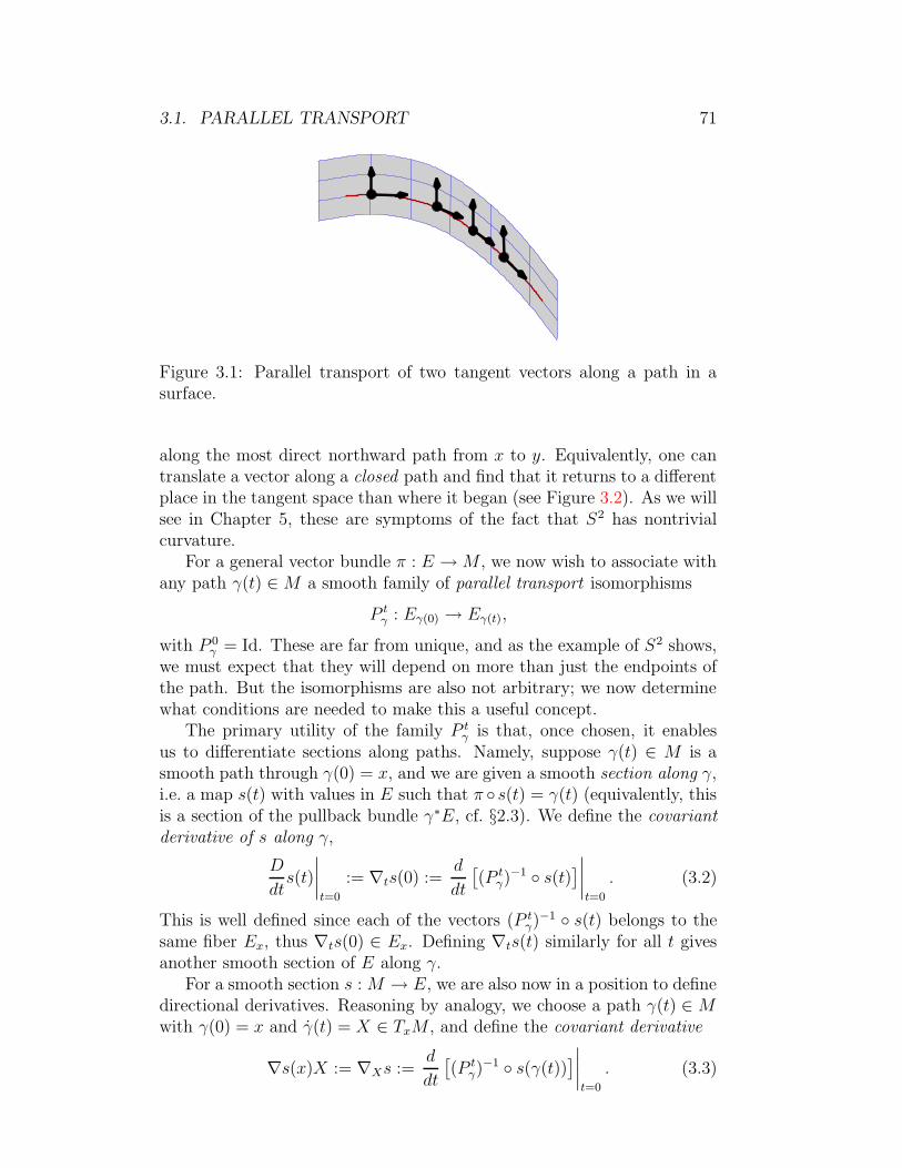
This leads to the idea of parallel transport, or parallel translation. Theeasiest example to think of is the tangent bundle of a submanifold M ⊂ Rm;for simplicity, picture M as a surface embedded in R3 (Figure 3.1). Forany vector X ∈ TxM at x ∈ M and a path γ(t) ∈ M with γ(0) = x, it’snot hard to imagine that the vector X is “pushed” along the path γ in anatural way, forming a smooth family of tangent vectors X(t) ∈ Tγ(t)M .In fact, this gives a smooth family of isomorphisms
P tγ : TxM → Tγ(t)M
with P 0γ = Id, where “smooth” in this context means that in any local
trivialization of TM → M near x, P tγ is represented by a smooth path of
matrices. The reason this is well defined is that M has a natural connec-tion determined by its embedding in R3; this is known as the Levi-Civitaconnection, and is uniquely defined for any manifold with a Riemannianmetric (see Chapter 4).
Notice that in general if γ(0) = x and γ(1) = y, the isomorphismP 1
γ : TxM → TyM may well depend on the path γ, not just its endpoints.One can easily see this for the example of M = S2 by starting X as avector along the equator and translating it along a path that moves firstalong the equator, say 90 degrees of longitude, but then makes a sharpturn and moves straight up to the north pole. The resulting vector Y
at the north pole is different from the vector obtained by transporting X
3.1. PARALLEL TRANSPORT 71
PSfrag replacements
γX(p0)
Mp0
v0
R4
C
xy
Ex
Ey
Figure 3.1: Parallel transport of two tangent vectors along a path in asurface.
along the most direct northward path from x to y. Equivalently, one cantranslate a vector along a closed path and find that it returns to a differentplace in the tangent space than where it began (see Figure 3.2). As we willsee in Chapter 5, these are symptoms of the fact that S2 has nontrivialcurvature.
For a general vector bundle π : E → M , we now wish to associate withany path γ(t) ∈ M a smooth family of parallel transport isomorphisms
P tγ : Eγ(0) → Eγ(t),
with P 0γ = Id. These are far from unique, and as the example of S2 shows,
we must expect that they will depend on more than just the endpoints ofthe path. But the isomorphisms are also not arbitrary; we now determinewhat conditions are needed to make this a useful concept.
The primary utility of the family P tγ is that, once chosen, it enables
us to differentiate sections along paths. Namely, suppose γ(t) ∈ M is asmooth path through γ(0) = x, and we are given a smooth section along γ,i.e. a map s(t) with values in E such that π s(t) = γ(t) (equivalently, thisis a section of the pullback bundle γ∗E, cf. §2.3). We define the covariantderivative of s along γ,
D
dts(t)
∣∣∣∣t=0
:= ∇ts(0) :=d
dt
[(P t
γ)−1 s(t)
]∣∣∣∣t=0
. (3.2)
This is well defined since each of the vectors (P tγ)
−1 s(t) belongs to thesame fiber Ex, thus ∇ts(0) ∈ Ex. Defining ∇ts(t) similarly for all t givesanother smooth section of E along γ.
For a smooth section s : M → E, we are also now in a position to definedirectional derivatives. Reasoning by analogy, we choose a path γ(t) ∈ M
with γ(0) = x and γ(t) = X ∈ TxM , and define the covariant derivative
∇s(x)X := ∇Xs :=d
dt
[(P t
γ)−1 s(γ(t))
]∣∣∣∣t=0
. (3.3)

72 CHAPTER 3. CONNECTIONS
PSfrag replacements
γX(p0)
M
p0
v0R4
C
xy
Ex
Ey
Figure 3.2: Parallel transport of a vector along a closed path in S2 ⊂ R3
leads to a different vector upon return.
Once again we are differentiating a path of vectors in the same fiber Ex,so ∇s(x)X ∈ Ex. We can now begin to deduce what conditions must beimposed on the isomorphisms P t
γ: first, we must ensure that the expression(3.3) depends only on s and X = γ(0), not on the chosen path γ. Let usassume this for the moment. Then for any vector field X ∈ Vec(M), thecovariant derivative defines another section ∇Xs : M → E. Any sensibleuse of the word “derivative” should require that the resulting map
∇s(x) : TxM → Ex
be linear for all x. This is not automatic; it imposes another nontrivialcondition on our definition of parallel transport. It turns out that fromthese two requirements, we will be able to deduce the most elegant anduseful definition of a connection for vector bundles.
3.2 Connections on fiber bundles
Before doing that, it helps to generalize slightly and consider an arbitraryfiber bundle π : E → M , with standard fiber F . Now parallel transportalong a path γ(t) ∈ M will be defined by a smooth family of diffeomor-phisms P t
γ : Eγ(0) → Eγ(t), and we define covariant derivatives again by for-mulas (3.2) and (3.3). Now however, we are differentiating paths throughthe fiber Ex
∼= F , which is generally not a vector space, so ∇s(x)X isnot in the fiber itself but rather in its tangent space Ts(x)(Ex) ⊂ Ts(x)E.Remember that the total space E is itself a smooth manifold, and has itsown tangent bundle TE → E.
3.2. FIBER BUNDLES 73
Definition 3.1. Let π : E → M be a fiber bundle. The vertical bundleV E → E is the subbundle of TE → E defined by
V E = ξ ∈ TE | π∗ξ = 0.
Its fibers VpE := (V E)p ⊂ TpE are called vertical subspaces.
Then VpE = Tp(Eπ(p)), so the vertical subbundle is the set of all vectorsin TE that are tangent to any fiber.
Exercise 3.2. Show that V E → E is a smooth real vector bundle ifπ : E → M is a smooth fiber bundle, and the rank of V E → E is thedimension of the standard fiber F .
By the above definition, the covariant derivative defines for each sections : M → E and x ∈ M a map
∇s(x) : TxM → Vs(x)E. (3.4)
We shall require the definition of parallel transport in fiber bundles tosatisfy two (not quite independent) conditions:
(i) The definition of ∇Xs in (3.3) is independent of γ except for thetangent vector γ(0) = X.
(ii) The map ∇s(x) : TxM → Vs(x)E is linear.
Proposition 3.3. Suppose π : E → M is a fiber bundle and for every pathγ(t) ∈ M there is a smooth family of diffeomorphisms P t
γ : Eγ(0) → Eγ(t)
satisfying P 0γ = Id and conditions (i) and (ii). Then for each x ∈ M and
p ∈ Ex, there is a unique linear injection
Horp : TxM → TpE
such that Horp(γ(0)) = ddt
P tγ(p)
∣∣t=0
for all paths with γ(0) = x. Moreover,the image of Horp is complementary to VpE in TpE.
Proof. Fix x0 ∈ M and p0 ∈ Ex0. Then for any path γ(t) ∈ M with
γ(0) = x0, the family of diffeomorphisms P tγ : Ex0
→ Eγ(t) is the flow ofsome vector field Y (t, p) on the total space of the pullback bundle γ∗E.Choosing any section s : M → E with s(x0) = p0 and writing F (t, p) =(P t
γ)−1(p), we have
∇γ(0)s =d
dtF (t, s(γ(t)))
∣∣∣∣t=0
=∂F
∂t(0, p0) + D2F (0, p0) Ts(γ(0))
= −Y (0, p0) + Ts(γ(0)),
74 CHAPTER 3. CONNECTIONS
thus
Horp0(γ(0)) =
d
dtP t
γ(p0)
∣∣∣∣t=0
= Y (0, p0) = Ts(γ(0)) −∇γ(0)s. (3.5)
This expression is clearly a linear function of γ(0). It is also injective since∇γ(0)s ∈ Vp0
E, and Ts(γ(0)) ∈ Vp0E if and only if γ(0) = 0, as we can see
by applying π∗. The same argument shows (im Horp0) ∩ Vp0
E = 0, andsince any non-vertical vector ξ ∈ Tp0
E \ Vp0E can be written as Ts(γ(0))
for some path γ and section s, clearly
im Horp0⊕Vp0
E = Tp0E.
The moral is that parallel transport, if defined properly, determinesfor every p ∈ E a horizontal subspace HpE := im Horp complementary tothe vertical subspace VpE. Conversely, it’s easy to see that choosing suchcomplimentary subspaces HpE determines P t
γ uniquely. This should besufficient motivation for the following definition.
Definition 3.4. A connection on the fiber bundle π : E → M is a smoothdistribution HE on the total space such that HE ⊕ V E = TE. For anyp ∈ E, the fiber HpE ⊂ TpE is called the horizontal subspace at p.
We can now recast all of the previous concepts in terms of horizontalsubspaces. Assume a connection (i.e. a horizontal subbundle) has beenchosen. Then for each x ∈ M and p ∈ Ex, the linear map π∗ : TpE →TxM restricts to an isomorphism HpE → TxM . Its inverse is called thehorizontal lift
Horp : TxM → HpE.
A path through the total space E is called horizontal if it is everywheretangent to HE. Then given x0 ∈ M and p0 ∈ Ex0
, any path γ(t) ∈ M
with γ(0) = x0 lifts uniquely to a horizontal path γ(t) ∈ E with γ(0) = p0.This path is similarly called the horizontal lift of γ, and its tangent vectorssatisfy
d
dtγ(t) = Horγ(t)(γ(t)).
By considering horizontal lifts for all possible p ∈ Ex0, we obtain naturally
the parallel transport diffeomorphisms P tγ : Ex0
→ Eγ(t). Finally, (3.5)yields a convenient formula for the covariant derivative with respect to anyvector X ∈ TxM ,
∇Xs = Ts(X) − Hors(x)(X).

3.3. VECTOR BUNDLES 75
Note that since π∗Ts(X) = X, the second term on the right is simply theprojection of Ts(X) to the horizontal subspace. We can express this moresimply by defining the vertical projection
K : TE → V E,
which maps each TpE to the vertical subspace VpE by projecting alongHpE. Then
∇Xs = K Ts(X), (3.6)
so the covariant derivative is literally the “vertical part” of the tangentmap. For a section s(t) ∈ E along a path γ(t) ∈ M , we have the analogousformula
∇ts(t) = K(s(t)). (3.7)
As one would expect, it is clear from this formula that s(t) is a horizontallift of γ(t) if and only if ∇ts ≡ 0.
The projection K : TE → V E is called a connection map, and it givesan equivalent definition for connections on fiber bundles.
Definition 3.5. A connection on the fiber bundle π : E → M is a smoothfiberwise linear map K : TE → V E such that K(ξ) = ξ for all ξ ∈ V E.
The two definitions are related by setting HE = ker K.
Exercise 3.6. Show that every smooth fiber bundle admits a connection.Hint: any local trivialization defines a natural connection in its neighbor-hood. Use a partition of unity to piece together the connection maps. (Seethe proof of Theorem 3.37 if you need more hints.)
Remark 3.7. The existence of connections for bundles on infinite dimen-sional manifolds is a far more intricate problem, because such manifoldsdo not generally admit smooth partitions of unity. However, more directconstructions of connections succeed in many interesting cases, such as forthe “manifolds of maps” defined in [Elı67].
3.3 Connections on vector bundles
3.3.1 Three definitions
For a vector bundle π : E → M , some minor changes in the previousdiscussion are appropriate in order to exploit the linear structure on thefibers. Most importantly, it is no longer enough for the parallel transportmaps P t
γ : Eγ(0) → Eγ(t) to be diffeomorphisms; they should be linearisomorphisms. We thus define a linear connection to be any connectionon the fiber bundle E → M for which the induced parallel transport is

76 CHAPTER 3. CONNECTIONS
linear. It will always be assumed that a connection on a vector bundle isa linear connection unless otherwise noted. We will prove the existence ofsuch objects later, in the context of principal bundles.
To see more concretely what linearity entails, observe that for any scalarλ ∈ F, there is a fiberwise linear map
mλ : E → E : v 7→ λv,
which is a diffeomorphism if λ 6= 0. Choose a path γ(t) ∈ M , labelx = γ(0), X = γ(0) ∈ TxM , and choose v ∈ Ex. Then for any linearconnection, we have P t
γ(λv) = mλ(Ptγ(v)), and differentiating at t = 0,
Horλv(X) = (mλ)∗ Horv(X).
This implies HλvE = (mλ)∗HvE. Though it may not be obvious just yet,this is enough of a criterion to identify linear connections. We shall provethis below, after giving two new equivalent definitions.
Definition 3.8. A connection on the vector bundle π : E → M is a smoothdistribution HE on the total space such that HE⊕V E = TE and for anyscalar λ ∈ F and v ∈ E,
HλvE = (mλ)∗HvE.
Observe that the vector space structure on each fiber Ex gives naturalisomorphisms
Vertv : Ex → VvE : w 7→d
dt(v + tw)
∣∣∣∣t=0
for each v ∈ Ex. It is thus appropriate to rewrite the projection K :TE → V E as a map K : TE → E that takes TvE to Eπ(v) and satisfiesK(Vertv(w)) = w for all w ∈ Eπ(v). This will be called a connection mapfor the vector bundle π : E → M . Setting ker K = HE, it is an easyexercise to verify that the following is now equivalent to Definition 3.8.
Definition 3.9. A connection on the vector bundle π : E → M is a smoothmap K : TE → E such that
1. For each v ∈ E, K defines a real linear map TvE → Eπ(v).
2. K(Vertv(w)) = w for all w ∈ Eπ(v).
3. For all scalars λ ∈ F, K (mλ)∗ = mλ K.
We now show that these new definitions are equivalent to the notion ofa linear connection defined above. The following lemma will be of use.

3.3. VECTOR BUNDLES 77
Lemma 3.10. Let V and W be real, normed vector spaces. Then any mapF : V → W that is differentiable at 0 and satisfies F (λv) = λF (v) for allscalars λ ∈ R and all v ∈ V is linear.
Proof. The key is to show that under this assumption, F is actually equalto its derivative at zero, dF (0) : V → W . Clearly F (0) = 0, so we canwrite
F (v) = dF (0)v + |v|η(v)
for some function η : V → W such that limv→0 η(v) = 0. Then
F (v) = limλ→0+
1
λF (λv) = lim
λ→0+
dF (0)λv + λ|v|η(λv)
λ
= dF (0)v + limλ→0+
|v|η(λv) = dF (0)v.
Remark 3.11. The vector spaces V and W need not be finite dimensional—in particular, they could be Banach spaces.
Proposition 3.12. If π : E → M is a vector bundle and K : TE → E
is a connection as defined above, then the induced parallel transport mapsP t
γ : Eγ(0) → Eγ(t) are linear (with respect to F).
Proof. For any path γ(t) ∈ M , denote γ(0) = x, γ(0) = X ∈ TxM , andchoose any v ∈ Ex, λ ∈ F. Denote by γ(t) ∈ E the horizontal lift of γ
with γ(0) = v, and similarly let γλ(t) ∈ E denote the horizontal lift withγλ(0) = λv. We have,
d
dtmλ(γ(t)) = (mλ)∗
d
dtγ(t) = (mλ)∗ Horγ(t)(γ(t))
= Horλγ(t)(γ(t))
=d
dtγλ(t),
hence γλ(t) ≡ λγ(t). This proves that the diffeomorphisms P tγ : Eγ(0) →
Eγ(t) satisfyP t
γ(λv) = λP tγ(v) (3.8)
for all λ ∈ F, and by Lemma 3.10, P tγ is real linear. If F = C, it is clearly
also complex linear since (3.8) holds for λ ∈ C.
As before, the covariant derivative of a section s : M → E in thedirection X ∈ TxM is defined by
∇Xs =d
dt
[(P t
γ)−1 s(γ(t))
]∣∣∣∣t=0
, (3.9)

78 CHAPTER 3. CONNECTIONS
where γ(0) = X, and ∇Xs can now be regarded as a vector in Ex. In lightof the new definition for the connection map K : TE → E, we have also
∇Xs = K Ts(X). (3.10)
Similar remarks apply to sections along paths.For any smooth section s : M → E and vector field X ∈ Vec(M), ∇Xs
now defines another section of E, while ∇s itself defines a smooth sectionof the bundle of real linear maps HomR(TM, E) = T ∗M ⊗R E. Using (3.9)and the fact that P t
γ is linear, one sees that the resulting map
∇ : Γ(E) → Γ(HomR(TM, E))
is also linear (with respect to F).In this context, we have the following version of the product rule:
Proposition 3.13. For any section s : M → E and smooth functionf : M → F,
∇(fs) = df(·)s + f∇s, (3.11)
where both sides are regarded as sections of HomR(TM, E).
This also follows easily from (3.9), using the linearity of parallel trans-port. Formula (3.11) is called a Leibnitz rule for the operator ∇; suchrelations appear naturally in any context that involves derivatives of bi-linear products. We’ll see more examples in Chapter 4 when we defineconnections on the tensor bundles associated with E.
Prop. 3.13 has a converse of sorts, which leads to a third equivalentdefinition for linear connections. Suppose we have a vector bundle π :E → M and an F-linear operator
D : Γ(E) → Γ(HomR(TM, E))
satisfying the Leibnitz rule D(fs) = df · s + fDs. We denote DXs :=Ds(x)X for X ∈ TxM .
Proposition 3.14. Given the map D above, there is a unique connectionon π : E → M such that D = ∇.
The proof is based on the observation that any two operators satisfyingthe same Leibnitz rule must differ by an operator which is tensorial :
Lemma 3.15. Suppose D, D′ : Γ(E) → Γ(HomR(TM, E)) are two F-linear operators that satisfy the Leibnitz rule (3.11) for all smooth functionsf : M → F and sections s ∈ Γ(E). Then the operator L : Vec(M)×Γ(E) →Γ(E) defined by
L(X, s) = DXs − D′
Xs
determines a bilinear bundle map TM ⊕ E → E. The map is real linearin TM and F-linear in E.
3.3. VECTOR BUNDLES 79
Proof. We must verify that L : Vec(M) × Γ(E) → Γ(E) is C∞-linear in s,i.e. that L(X, fs) = fL(X, s) for all f ∈ C∞(M, F). Indeed,
L(X, fs) = DX(fs) − D′
X(fs) = df(X)s + fDXs − df(X)s − fD′
Xs
= f(DXs − D′
Xs) = fL(X, s).
Clearly also L(fX, s) = fL(X, s) for all smooth real-valued functions f .This shows that for each x0 ∈ M , the value of L(X, s)(x0) depends onlyon X(x0) and s(x0).
Proof of Prop. 3.14. Uniqueness is easy: if there is such a connection, thenthe resulting horizontal lift maps Horv : TxM → TvE for v ∈ Ex mustsatisfy
Horv(X) = Ts(X) − Vertv(DXs)
for all X ∈ TxM and s ∈ Γ(E) with s(x) = v. To prove existence, we mustverify that the right hand side of this expression gives a well defined linearmap TxM → TvE, regardless of the choice of section with s(x) = v.
We show this by choosing another connection K, which induces a covari-ant derivative operator ∇ : Γ(E) → Γ(HomR(TM, E)), satisfying the Leib-nitz rule (3.11). By Lemma 3.15, there is a bundle map L : TM ⊕E → E
such that L(X, s) ≡ ∇Xs − DXs, and for X ∈ TxM , we have
Ts(X) − Vertv(DXs) = Ts(X) − Vertv(∇Xs) + Vertv(L(X, v))
= Horv(X) + Vertv(L(X, v)),
where Horv : TxM → TvE denotes the horizontal lift map defined by K.The right hand side now depends only on X and v, and gives a well definedlinear injection TxM → TvE. There is a unique connection K such thatthis map is Horv for each v ∈ Ex, and by construction, ∇ = D.
We are now ready for the “quick and dirty” definition of linear connec-tions that is most commonly found in modern introductions to differentialor Riemannian geometry. Prop. 3.14 shows that it is equivalent to ourprevious two definitions.
Definition 3.16. A connection on the vector bundle π : E → M is anF-linear operator
∇ : Γ(E) → Γ(HomR(TM, E))
satisfying the Leibnitz rule
∇(fs) = df(·)s + f∇s
for all functions f ∈ C∞(M, F) and sections s ∈ Γ(E).

80 CHAPTER 3. CONNECTIONS
3.3.2 Christoffel symbols
Let π : E → M denote a vector bundle, and choose a local trivialization
Φ : E|U → U × Fm
over some open subset U ⊂ M . Using the trivialization we can identifysections s : U → E|U with maps U → F
m. Then Φ determines a naturalconnection on E|U , for which the covariant derivative acts on sections s :U → Fm by s 7→ ds.
Given another connection ∇ : Γ(E) → Γ(HomR(TM, E)), Lemma 3.15implies that ∇ differs from this natural connection on E|U by a bilinearbundle map
ΓΦ : (TM ⊕ E)|U → EU ;
that is, for any section s ∈ Γ(E|U) expressed as a map U → Fm, we have
∇s(x)X = ds(x)X + ΓΦ(X, s(x)) for x ∈ U . (3.12)
Note that ΓΦ is real linear in the first factor and F-linear in the second.It must be emphasized that ΓΦ is not globally defined, and it depends onthe choice of trivialization. Of course we’re being somewhat sloppy withnotation; one can think of ΓΦ either as a bundle map on (TM ⊕E)|U , or—since we’re really working in a trivialization—as a bilinear map TM |U ×Fm → Fm.
One more often sees ΓΦ expressed in local coordinates as a set of locallydefined functions with three indices. Assume U admits a coordinate system(x1, . . . , xn); this then determines a framing (∂1, . . . , ∂n) of the tangentbundle TM |U , i.e. a set of linearly independent vector fields that spanthe tangent space at each point. There is similarly a canonical framing(e(1), . . . , e(m)) of E|U determined by Φ. Then the functions Γa
ib : U → F
are defined by
ΓΦ(∂i, e(b)) = Γaibe(a),
so that for any X = X i∂i ∈ TxM and v = vbe(b) ∈ Ex, we have
ΓΦ(X, v) = ΓΦ(X i∂i, vbe(b)) = X ivbΓΦ(∂i, e(b)) = Γa
ibXivbe(a),
i.e. (ΓΦ(X, v))a = ΓaibX
ivb. A section s : U → E|U can now be expressedas s = sae(a) for a set of m functions sa : U → F, and writing ∇i := ∇∂i
,equation (3.12) becomes
(∇is)a = ∂is
a + Γaibs
b. (3.13)
In this context the functions Γaib are called Christoffel symbols. Standard
treatments of general relativity usually define connections purely in terms

3.3. VECTOR BUNDLES 81
of the Christoffel symbols, while the covariant derivative is defined by(3.13).
In order for this definition of a connection to make sense, one musthave the right notion of how the symbols Γa
ib “transform” with respect tochanges in coordinates and local trivializations.
Exercise 3.17. Given a bundle π : E → M and a sufficiently smallopen set U ⊂ M , use a coordinate system (x1, . . . , xn) and a framing(e(1), . . . , e(m)) to identify E|U with the trivial bundle V × Fm, where V isan open subset of Rn. Suppose Γa
ib are the corresponding Christoffel sym-bols for some connection ∇ on E. Then another choice of coordinates andframing can be expressed by smooth functions
V → Rn : (x1, . . . , xn) 7→ (x1, . . . , xn)
V → Rm : (x1, . . . , xn) 7→ e(1) = (e1
(1), . . . , em(1))
...
V → Rm : (x1, . . . , xn) 7→ e(m) = (e1
(m), . . . , em(m))
Let Γaib denote the Christoffel symbols of ∇ with respect to (x1, . . . , xn)
and (e1, . . . , em). Derive the transformation formula
Γaib =
∂xj
∂xiec(b)Γ
ajc +
∂xj
∂xi
∂
∂xjea(b).
As a special case when E = TM , show that this becomes
Γijk =
∂xp
∂xj
∂xq
∂xkΓi
pq +∂xp
∂xj
∂
∂xp
(∂xi
∂xk
).
Remark 3.18. The definitions we’ve stated are not quite strict enough todefine connections on an infinite dimensional Banach space bundle. Sup-pose for instance that the base M is a Banach manifold that looks locallylike the Banach space X, and E → M is a bundle with fibers isomorphicto a Banach space Y. One must now explicitly require that for any choiceof smooth chart ϕ : U → X and local trivialization Φ : E|U → U × Y,there is a smooth Christoffel map
ΓΦ : U → L(X ⊗R Y,Y).
In the infinite dimensional case, this is stricter than simply asking for themap (x, X, v) 7→ ΓΦ(x, X, v) to be smooth; we saw an analogous situationin the definition of a Banach space bundle (see Definition 2.60). This tech-nical requirement is needed in order that the covariant derivative shoulddefine a continuous linear map
∇ : Γ(E) → Γ(HomR(TM , E)).
We will continue to assume for the remainder of this discussion that allobjects are finite dimensional unless otherwise noted.
82 CHAPTER 3. CONNECTIONS
3.3.3 Connection 1-forms
As an alternative to the Christoffel symbols, one can express covariantderivatives in local trivializations via matrix-valued 1-forms. If Uα ⊂ M isan open subset and Φα : E|Uα
→ Uα × Fm is a trivialization, we can writeany smooth section s ∈ Γ(E) over Uα via the smooth map sα : Uα → Fm
such that
Φα s(x) = (x, sα(x)). (3.14)
Then for x ∈ Uα and X ∈ TxM , the covariant derivative of s in the directionof X can always be written in the form
(∇Xs)α = dsα(X) + Aα(X)sα(x), (3.15)
where Aα is an m-by-m matrix-valued 1-form. The existence of such a1-form is another easy consequence of Lemma 3.15; in fact, it’s not hardto express Aα directly in terms of the Christoffel symbols:
Exercise 3.19. Choosing coordinates (x1, . . . , xn), let Ai = Aα(∂i) anddenote the entries of this m-by-m matrix by (Ai)
ab. Show that (Ai)
ab = Γa
ib.
We call Aα the connection 1-form for ∇ with respect to the trivializationΦα. This leads to yet another definition of connections that is somewhatuntidy but popular in the physics world: a connection is a choice of m-by-mmatrix-valued 1-forms Aα over Uα corresponding to each local trivializationΦα and satisfying the appropriate transformation property with respect tochange of trivialization (see the exercise below).
Exercise 3.20. If g = gβα : Uα ∩ Uβ → GL(m, F) is the transition maprelating two trivializations Φα and Φβ, prove the transformation formula
Aα(X) = g−1Aβ(X)g + g−1dg(X). (3.16)
Physicists refer to (3.16) as a gauge transformation, alluding to theimportant role that connection 1-forms play in quantum field theory: inthat context they are called gauge fields, and they serve to model elemen-tary particles such as photons and other “gauge bosons” that mediate thefundamental forces of nature. The choice of the letter A to denote a con-nection form is in fact motivated by physics, where the vector potential ofclassical electromagnetic field theory (conventionally denoted by A) canbe interpreted as a connection form for a trivial Hermitian line bundle.
There is another reason to use connection 1-forms rather than Christof-fel symbols when the vector bundle has extra structure. In this case it’sappropriate to restrict attention to a particular class of connections, and itturns out that this restriction can be expressed elegantly via the connectionforms.

3.3. VECTOR BUNDLES 83
Definition 3.21. Let π : E → M be a vector bundle with a G-structure,for some Lie group G. Then a connection ∇ on E is called G-compatibleif all parallel transport isomorphisms respect the G-structure: this meansthat for any sufficiently short path γ(t) ∈ M , the maps P t
γ : Eγ(0) → Eγ(t)
can be written in a G-compatible trivialization as
P tγ : F
m → Fm : v 7→ g(t)v
for some smooth map g(t) ∈ G with g(0) =.
The definition seems less abstract when we apply it to particular struc-tures: e.g. for G = O(m) or U(m), the structure in question is a bundlemetric, and ∇ is called a metric connection if all parallel transport mapsare isometries. The terms complex connection and symplectic linear con-nection can be defined analogously.
The existence of G-compatible connections will follow from our discus-sion of principal bundles below. For now, we take existence as a given andexamine the consequences for connection 1-forms. Suppose in particularthat π : E → M is a vector bundle of rank m with a G-structure, for someLie subgroup G ⊂ GL(m, F)—as a concrete example to keep in mind, thereader may assume G = O(m) and the G-structure is a bundle metric.Assume Φα : E|Uα
→ Uα × Fm is a G-compatible trivialization (e.g. anorthonormal frame), ∇ is a G-compatible connection, and γ(t) is a smoothpath in M with γ(0) = x ∈ Uα. Let s(t) ∈ Eγ(t) be a section along γ whichis parallel, i.e. ∇ts ≡ 0. Then (3.15) gives
sα(t) + Aα(γ(t))s(t) = 0. (3.17)
Since the trivialization and connection are both G-compatible, the factthat s(t) is parallel also implies we can write sα(t) = g(t)sα(0) for somesmooth path of matrices g(t) ∈ G with g(0) =
, thus Aα(γ(0)) = −g(0).
This cannot be just any arbitrary m-by-m matrix: the tangent space T G
is generally a proper subspace of the space of all matrices, called the Liealgebra
T G = g ⊂ Fm×m
of the group G (see Appendix B). For example if G = O(m), then g =o(m) is the space of antisymmetric matrices. This leads to a convenientcharacterization of G-compatible connections.
Proposition 3.22. If E → M is a vector bundle with a G-structure and∇ is a connection on E, then ∇ is G-compatible if and only if for everyG-compatible trivialization Φα, the corresponding connection 1-form
Aα ∈ Ω1(Uα, Fm×m)
takes values in the Lie algebra g ⊂ Fm×m of G.

84 CHAPTER 3. CONNECTIONS
Proof. The argument above proves that G-compatibility implies Aα ∈Ω1(Uα, g). Conversely if the latter is true and v(t) ∈ Eγ(t) is any parallelsection along a smooth path γ(t) ∈ Uα, (3.17) implies
vα(t) = −Aα(γ(t))vα(t).
The result now follows from Exercise 3.23 below.
Exercise 3.23. For any matrix Lie group G ⊂ GL(m, F) and a smoothpath of matrices A(t) ∈ g, show that the unique solution Φ(t) ∈ Fm×m tothe initial value problem
Φ(t) = A(t)Φ(t),
Φ(0) =
satisfies Φ(t) ∈ G. Hint: show first that for any A ∈ g and B ∈ G,AB ∈ TBG; then Φ(t) is an orbit of a time-dependent vector field on G.
3.3.4 Linearization of a section at a zero
The following observation is trivial but useful:
Proposition 3.24. Suppose π : E → M is a smooth vector bundle ands : M → E is a smooth section with s(x) = 0. Then the linear map
∇s(x) : TxM → Ex
is independent of the choice of connection.
The proof is easy if we view it in the right context: recall that every vec-tor bundle has a preferred embedding M → E, the zero section. One seeseasily from the condition HλvE = (mλ)∗HvE that horizontal subspaces inTE are always tangent to M—thus every linear connection looks identicalalong the zero section. Put another way, at any point x ∈ M ⊂ E, whichwe view as lying either in M or in the zero section of E, there is a naturalisomorphism
TxE = Ex ⊕ TxM,
and any connection map K : TE → E defines the projection to the firstfactor. Thus the expression ∇s(x) = K ds(x) is invariantly defined aslong as s(x) = 0.
We call ∇s(x) : TxM → Ex the linearization of s at x ∈ s−1(0), andsince it doesn’t depend on ∇, we may as well denote
ds(x) := ∇s(x).
The definition of ds(x) via a connection is often convenient, but not nec-essary, as the next result shows.

3.3. VECTOR BUNDLES 85
Proposition 3.25. Suppose the section s : M → E has a zero at x, and wechoose a trivialization on some neighborhood x ∈ U ⊂ M so as to identifysections with maps f : U → Fm. Then the linearization at x is expressed inthis trivialization as df(x) : TxM → Fm, and the resulting map TxM → Ex
is independent of the chosen trivialization.
Proof. Differentiation in a trivialization can be viewed simply as covariantdifferentiation with respect to a connection determined by the trivializa-tion. The result then follows from Proposition 3.24. (Alternatively, onecan prove this by a direct computation without mentioning connections atall. Try it if you have a moment to spare.)
In the special case E = TM , there is a nice way to write the lineariza-tion without any arbitrary choices. A section in this case is a vector fieldX ∈ Vec(M), and it determines a flow ϕt : M → M ; these diffeomor-phisms may not be globally defined if M is noncompact, but they are atleast defined for t close to 0 and x in a neighborhood of any point x0 withX(x0) = 0. In particular, ϕt(x0) = x0 for all t, and there is a correspondingsmooth family of linear maps
dϕt(x0) : Tx0M → Tx0
M.
These determine a differentiable path through the identity in the vectorspace End(Tx0
M), and as it turns out,
d
dtdϕt(x0)
∣∣∣∣t=0
= dX(x0). (3.18)
Exercise 3.26. Use a coordinate system around x0 to prove (3.18).
Another example of this construction is the Hessian of a smooth func-tion f : M → R at a critical point. In general, the first derivatives off are easily characterized via the differential df ∈ Ω1(M), but without aconnection there is no such simple coordinate-invariant construction thatdescribes its second derivatives. If a connection ∇ is chosen on T ∗M , thenthis information is of course contained in the tensor field ∇df ∈ Γ(T 0
2 M).We observe now that for all critical points x ∈ M of f , i.e. points wheredfx : TxM → R is the zero map, the bilinear form
∇dfx : TxM × TxM → R
doesn’t depend on the choice of connection. We call this bilinear map theHessian of f at x.
Proposition 3.27. For any critical point x of f ∈ C∞(M), the Hessian∇dfx is symmetric, i.e. ∇dfx(X, Y ) = ∇dfx(Y, X) for all X, Y ∈ TxM .
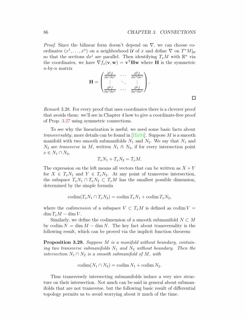
86 CHAPTER 3. CONNECTIONS
Proof. Since the bilinear form doesn’t depend on ∇, we can choose co-ordinates (x1, . . . , xn) on a neighborhood U of x and define ∇ on T ∗M |Uso that the sections dxj are parallel. Then identifying TxM with Rn viathe coordinates, we have ∇fx(v,w) = vTHw where H is the symmetricn-by-n matrix
H =
∂2f
∂x1∂x1 · · · ∂2f
∂xn∂x1
.... . .
...∂2f
∂x1∂xn · · · ∂2f
∂xn∂xn
.
Remark 3.28. For every proof that uses coordinates there is a cleverer proofthat avoids them: we’ll see in Chapter 4 how to give a coordinate-free proofof Prop. 3.27 using symmetric connections.
To see why the linearization is useful, we need some basic facts abouttransversality ; more details can be found in [Hir94]. Suppose M is a smoothmanifold with two smooth submanifolds N1 and N2. We say that N1 andN2 are transverse in M , written N1 t N2, if for every intersection pointx ∈ N1 ∩ N2,
TxN1 + TxN2 = TxM.
The expression on the left means all vectors that can be written as X + Y
for X ∈ TxN1 and Y ∈ TxN2. At any point of transverse intersection,the subspace TxN1 ∩ TxN2 ⊂ TxM has the smallest possible dimension,determined by the simple formula
codim(TxN1 ∩ TxN2) = codim TxN1 + codim TxN2,
where the codimension of a subspace V ⊂ TxM is defined as codim V =dim TxM − dim V .
Similarly, we define the codimension of a smooth submanifold N ⊂ M
by codim N = dim M − dim N . The key fact about transversality is thefollowing result, which can be proved via the implicit function theorem:
Proposition 3.29. Suppose M is a manifold without boundary, contain-ing two transverse submanifolds N1 and N2 without boundary. Then theintersection N1 ∩ N2 is a smooth submanifold of M , with
codim(N1 ∩ N2) = codim N1 + codim N2.
Thus transversely intersecting submanifolds induce a very nice struc-ture on their intersection. Not much can be said in general about subman-ifolds that are not transverse, but the following basic result of differentialtopology permits us to avoid worrying about it much of the time.

3.3. VECTOR BUNDLES 87
Proposition 3.30. Given any two smooth submanifolds N1 ⊂ M andN2 ⊂ M without boundary, one can move N1 by an arbitrarily small per-turbation so that N1 t N2.
One often abbreviates this by saying that generic submanifolds intersecttransversely.1 We refer to [Hir94] for the proof, but mention a special casein which the result is easy to visualize: suppose N1 and N2 are smoothcurves in the plane M = R2. Then transversality can only fail if N1 and N2
have a point of tangent intersection. One can always change the directionof N1 just slightly to kill the tangency.
Notice that transverse intersection points are impossible unless dim N1+dim N2 ≥ dim M ; in this case Proposition 3.30 says that one can perturbN1 so that the two submanifolds have no intersection at all. This is thecase for instance with a pair of smooth curves in R3. It is also the reasonwhy airplanes generically do not crash into each other.
Now, suppose π : E → M is a smooth vector bundle of rank m overan n-dimensional manifold. Any smooth section s : M → E then definesa submanifold s(M) ⊂ E of codimension m, and in particular there isthe special submanifold M ⊂ E defined by the zero section. Using thisnotation, we say that a section s ∈ Γ(E) is transverse to the zero sectionif s(M) t M .
Theorem 3.31. A smooth section s : M → E is transverse to the zerosection if and only if for every zero x ∈ s−1(0), the linearization ds(x) :TxM → Ex is a surjective map. In this case the zero set s−1(0) ⊂ M
is a smooth submanifold, with dimension equal to dimR ker ds(x) for anyx ∈ s−1(0).
Proof. Identify M with the zero section so that we can treat it as a sub-manifold of E. Then if s(x) = 0, transversality is achieved if and onlyif
im Ts|TxM + TxM = TxE.
Identifying TxE with Ex⊕TxM in the canonical way, it’s equivalent that theprojection K : TxE → Ex should map im Ts|TxM onto Ex, which meansK Ts|TxM = ∇s(x) is surjective. The dimension formula is a simpleexercise.
Note that by Proposition 3.30, sections s : M → E are genericallytransverse to the zero section.
1The word “generic” has a variety of precise meanings in different mathematicalcontexts, but it always refers to a situation in which one expects things to appear acertain way, and the alternative is somehow an exceptional case. For example, a genericpair of vectors in R2 is linearly independent, just as a generic matrix is invertible. Givena non-generic situation, one can always achieve the generic case by a small perturbation.

88 CHAPTER 3. CONNECTIONS
Remark 3.32. One can alternatively use a more straightforward implicitfunction theorem argument to show that s−1(0) ⊂ M is a smooth subman-ifold if and only if ds(x) is surjective for all x ∈ s−1(0). A similar statementis true for smooth maps f : Rn → RN ; this case can be reduced to thatone by choosing local coordinates and trivializations.
3.4 Connections on principal bundles
Before plunging into the definitions for principal connections, let us providesome motivation. As we saw in Section 2.8, one can always use a principalbundle to encode the essential data of a vector bundle and any additionalstructure that’s attached to it. Thus instead of dealing with the assortedvariety of structures such as bundle metrics or symplectic structures thatmight be associated with a vector bundle, one can describe all of thesein a unified way by identifying the structure group and defining the cor-responding frame bundle. A connection on the frame bundle will inducea connection on the original bundle, with parallel transport that respectsany special structure that may be present. Indeed, the same is true formore general fiber bundles with finite dimensional structure groups. Thusthe construction of connections on principal bundles has implications thatgo well beyond the study of principal bundles themselves.
3.4.1 Definition
Let G be a Lie group, and π : E → M a principal G-bundle. Recallthat the fibers of E have intrinsic structure in the form of a smooth fiberpreserving right group action
E × G → E : (p, g) 7→ pg,
which is free and transitive on each fiber. A connection on E → M iscalled a principal connection if the parallel transport diffeomorphisms P t
γ :Eγ(0) → Eγ(t) are G-equivariant, that is,
P tγ(pg) = P t
γ(p)g
for all p ∈ Eγ(0) and g ∈ G.
As usual, this first definition is conceptually simple but hard to workwith in practice, so we’ll give some equivalent definitions. The first stepis to determine the implications of G-equivariance for the horizontal sub-bundle HE ⊂ TE. Each g ∈ G determines a fiber preserving diffeomor-phism Rg : E → E : p 7→ pg. Choose a path γ(t) ∈ M with γ(0) = x,γ(0) = X ∈ TxM , and let p ∈ Ex. Given a principal connection, the

3.4. PRINCIPAL BUNDLES 89
horizontal lift isomorphisms have the property
Horpg(X) =d
dtP t
γ(pg)
∣∣∣∣t=0
=d
dtRg P t
γ(p)
∣∣∣∣t=0
= (Rg)∗d
dtP t
γ(p)
∣∣∣∣t=0
= (Rg)∗ Horp(X).
We conclude HpgE = (Rg)∗HpE. Conversely, any fiber bundle connectionwith this property defines G-equivariant parallel transport; one can provethis along the same lines as for vector bundles. The following is thereforean equivalent definition for principal connections.
Definition 3.33. A connection on the principal fiber bundle π : E → M
with structure group G is a smooth distribution HE on the total spacesuch that HE ⊕ V E = TE and for any g ∈ G and p ∈ E,
HpgE = (Rg)∗HpE.
3.4.2 Global connection 1-forms
The connection map K : TE → V E for a principal G-bundle E → M
can be put in a simplified form by noting that in this situation the verticalbundle V E → E is necessarily trivial; in fact, we will now show that it hasa preferred trivialization. Recall that every Lie group G has an associatedLie algebra g, which is the tangent space TeG with a bracket operation[ , ] : g × g → g induced by the group multiplication on G. There is alsoa so-called exponential map
exp : g → G
defined such that for each X ∈ g, t 7→ exp(tX) is the unique Lie grouphomomorphism R → G with d
dtexp(tX)
∣∣t=0
= X. For matrix groups G ⊂GL(m, F) in particular, where g is naturally a subspace of Fm×m, it turnsout that [A,B] = AB−BA and exp(tA) = etA is defined by the familiarpower series expansion. (These concepts are reviewed in Appendix B). Nowif E → M is a principle G-bundle, the right action E × G → E defines anatural bundle isomorphism
E × g → V E : (p, X) 7→ X(p) =d
dt(p exp(tX))
∣∣∣∣t=0
. (3.19)
The vertical vector field on E defined by X(p) is called the fundamentalvector field determined by X ∈ g.
If HE ⊂ TE is a principal connection, we can use the isomorphism(3.19) to rewrite the connection map K : TE → V E as a g-valued 1-form
A ∈ Ω(E, g) := Γ(Hom(TE, E × g)),

90 CHAPTER 3. CONNECTIONS
giving for each p ∈ E a linear map Ap : TpE → g, such that ker Ap =HpE. Since K is a projection onto V E, A has the property A(X(p)) = X
for all p ∈ E and X ∈ g. Recall also that HE is required to satisfyHpgE = (Rg)∗HpE for all p ∈ E and g ∈ G. To express the consequence ofthis condition for A, we need the following fact about fundamental vectorfields. Recall from Appendix B the definition of the adjoint representationAd : G → Aut(g) : g 7→ Adg, which for matrix groups takes the form
AdB(A) = BAB−1.
Lemma 3.34. If g ∈ G and X ∈ g, then
(Rg)∗X = Adg−1(X).
Proof. For p ∈ E, compute
((Rg)∗X)(pg) =d
dtRg(p exp(tX))
∣∣∣∣t=0
=d
dtp exp(tX)g
∣∣∣∣t=0
=d
dtpg
(g−1 exp(tX)g
)∣∣∣∣t=0
=d
dtpg exp (t Adg−1(X))
∣∣∣∣t=0
= Adg−1(X)(pg).
Any vector ξ ∈ TpE can be written uniquely as ξ = ξh + X(p) whereξh ∈ HpE and X ∈ g. Then A(ξ) = X, and HpgE = (Rg)∗HpE implies
R∗
gA(ξ) = A((Rg)∗(ξh + X(p))) = A(Adg−1(X)(pg)) = Adg−1(X)
= Adg−1 A(ξ).
Conversely, it’s not hard to show (Exercise 3.36 below) that any g-valued1-form satisfying these conditions defines a principal connection by HE =ker A. We therefore have a useful new definition for principal connections.
Definition 3.35. A connection on the principal fiber bundle π : E → M
with structure group G is a smooth g-valued 1-form A ∈ Ω(E, g) such that:
(i) A(X(p)) = X for all X ∈ g and p ∈ E,
(ii) (Rg)∗A = Adg−1 A for all g ∈ G.
Exercise 3.36. Show that if A ∈ Ω(E, g) satisfies the conditions in Def-inition 3.35, then the distribution HE = ker g satisfies the conditions inDefinition 3.33.
Defining connections in terms of global 1-forms has several advantages,the first of which is that proving existence is now a simple exercise withpartitions of unity.

3.4. PRINCIPAL BUNDLES 91
Theorem 3.37. Every principal fiber bundle admits a connection.
Proof. Assume π : E → M is a principal G-bundle and (Uα, Φα) is asystem of local trivializations. Since M is paracompact, we can replaceUα with a locally finite refinement and choose a smooth partition ofunity ϕα. Each trivialization Φα : π−1(Uα) → Uα ×G defines an obviousnotion of G-equivariant parallel transport within Uα, and thus a connectionAα ∈ Ω(Uα, g) over Uα. We use these to define a global g-valued 1-form
A =∑
α
ϕαAα.
We claim that A is a connection. For X ∈ g, x ∈ M and p ∈ Ex, we have
A(X(p)) =∑
α
ϕα(x)Aα(X(p)) =∑
α
ϕα(x)X = X.
Likewise for g ∈ G,
(Rg)∗A =∑
α
ϕα · (Rg)∗Aα =∑
α
ϕα · Adg−1 Aα
= Adg−1
∑
α
ϕαAα = Adg−1 A,
proving the claim.
3.4.3 Frame bundles and linear connections
Theorem 3.37 is more than an existence result for principal connections:it also implies the existence of compatible connections on any fiber bundlewith a finite dimensional structure group. We now prove this in particularfor linear connections on vector bundles.
Recall from Example 2.81 in Chapter 2 that for every vector bundleE → M with structure group G, there is an associated frame bundleF GE → M , a principal G-bundle whose fibers are spaces of preferredbases for the fibers of E. Each element of the fiber F GEx thus definesa unique isomorphism Fm → Ex, so there is a smooth, fiber preservinginclusion map
Ψ : F GE → Hom(M × Fm, E)
taking each p ∈ F GEx to the corresponding isomorphism Ψ(p) : Fm → Ex.Treating any g ∈ G as a linear map on F
m, we have
Ψ(pg) = Ψ(p) g.
There is also a a “vertical tangent map”
V Ψ : V F GE → Hom(M × Fm, E)
92 CHAPTER 3. CONNECTIONS
such that for any smooth path p(t) ∈ F GEx,
V Ψ(p(t)) =d
dtΨ(p(t)),
where the right hand side is interpreted as the derivative of a smooth pathin the vector space Hom(Fm, Ex).
Theorem 3.38. Suppose π : E → M is a smooth vector bundle, G isa Lie group and E → M is equipped with a G-structure. Then the set ofG-compatible linear connections on E is in one-to-one correspondence withthe set of principal connections on the frame bundle F GE → M .
In particular, given a connection on F GE there is a unique connectionon E such that for every smooth path γ(t) in M , the parallel sections ofE along γ are of the form v(t) = Ψ(s(t))v, where s(t) is a parallel sectionof F GE along γ and v ∈ Fm is constant. This connection on E is G-compatible, and for any smooth section s(t) ∈ F GEγ(t) and smooth mapv(t) ∈ Fm, the section Ψ(s)v ∈ Eγ(t) satisfies
∇t(Ψ(s)v) = V Ψ(∇ts)v + Ψ(s)∂tv. (3.20)
Proof. If a connection on F GE is given, then for a smooth path γ(t) ∈ M
with γ(0) = x and γ(t) = X ∈ TxM , we pick any frame p ∈ F GEx anddefine a horizontal lift map by
HorΨ(p)v : TxM → TΨ(p)vE : X 7→d
dtΨ(P t
γ(p))v
∣∣∣∣t=0
for every v ∈ Fm. Any other choice of p ∈ F GEx gives the same resultdue to the G-equivariance of P t
γ. The images of all the horizontal lift mapsdefine a distribution HE, which is clearly a fiber bundle connection on E.The fact that it is G-compatible follows from the observation that eachp ∈ F GEx defines a G-compatible trivialization of E along γ by
Eγ(t) → γ(t) × Fm : v 7→
(γ(t),
[Ψ
(P t
γ(p))]−1
(v))
;
in this trivialization, parallel transport in E along γ is the identity. Notethat since G acts linearly on Fm, the resulting connection on E is auto-matically linear.
Conversely if E has a G-compatible connection with parallel transportQt
γ : Eγ(0) → Eγ(t) along γ, there is a unique principal connection on F GE
such that for each p ∈ FEx, the expression
Ψ(p(t))v = Qtγ Ψ(p)v
extends p to a parallel section p(t) of F GE along γ.
3.4. PRINCIPAL BUNDLES 93
Equation (3.20) now follows from the definition of covariant differenti-ation along a path: we have
∇t(Ψ(s)v)|t=0 =d
dt(Qt
γ)−1 (Ψ (s(t))v(t))
∣∣∣∣t=0
=d
dt
[Ψ
([P t
γ]−1(s(t))
)v(t)
]∣∣∣∣t=0
= V Ψ
(d
dt(P t
γ)−1(s(t))
∣∣∣∣t=0
)v(0) + Ψ(s(0))
d
dtv(t)
∣∣∣∣t=0
= V Ψ(∇ts)|t=0 · v(0) + Ψ(s(0))v(0).
Corollary 3.39. Every smooth vector bundle with a G-structure admits aG-compatible connection.
This proves the existence of metric connections, complex connectionsand linear symplectic connections on every bundle with the correspondingstructure. The beauty of the principal bundle formalism is that all of theseexistence results follow from a single construction. We obtain also a conve-nient relation between the global connection 1-form A ∈ Ω1(F GE, g) andthe local connection forms Aα ∈ Ω1(Uα, g) corresponding to trivializations.
Proposition 3.40. Suppose A ∈ Ω1(F GE, g) is a connection on F GE. LetΦα : E|Uα
→ Uα ×Fm denote any local trivialization of E, with correspond-ing local connection 1-form Aα ∈ Ω1(Uα, g), and denote by sα : Uα → F GE
the unique local section of F GE such that
Φ−1α (x,v) = Ψ(sα(x))v.
ThenAα = s∗αA
Proof. Let x ∈ Uα and X ∈ TxM . The form Aα is defined such that forany smooth map v : Uα → Fm,
∇X(Ψ(sα)v) = Ψ(sα) (dv(X) + Aα(X)v) ,
whereas (3.20) gives
∇X(Ψ(sα)v) = V Ψ(∇Xsα)v + Ψ(sα)dv(X),
implying V Ψ(∇Xsα)v = Ψ(sα)Aα(X)v. Recalling from (3.19) the defini-tion of the fundamental vector field, we have
∇Xsα = K(Tsα(X)) = A(Tsα(X))(sα(x)) = s∗αA(X)(sα(x))
=d
dt[sα(x) exp(ts∗αA(X))]
∣∣∣∣t=0
,
94 CHAPTER 3. CONNECTIONS
and thus
V Ψ(∇Xsα)v =d
dtΨ (sα(x) exp(ts∗αA(X)))v
∣∣∣∣t=0
= Ψ(sα(x))d
dtexp(ts∗αA(X))v
∣∣∣∣t=0
= Ψ(sα(x)) s∗αA(X)v.
We conclude s∗αA(X) = Aα(X).
Remark 3.41. One can define frame bundles not just for vector bundlesbut for any smooth fiber bundle E → M with a finite dimensional struc-ture group G: the frame bundle is then a principal G-bundle whose fibersconsist of preferred diffeomorphisms between fibers of E and the standardfiber F . With this notion, the existence result above generalizes nicelyto a construction of G-compatible connections on any such fiber bundle.The only limitation is that this argument applies only to fiber bundleswith finite dimensional structure groups—extending it beyond this settingwould require considerably more analytical effort. Fortunately one can of-ten prove existence by more direct means in particular cases of interest,e.g. symplectic fibrations (cf. [MS98]).
References
[Elı67] H. I. Elıasson, Geometry of manifolds of maps, J. Differential Geometry 1
(1967), 169–194.
[Hir94] M. W. Hirsch, Differential topology, Springer-Verlag, New York, 1994.
[MS98] D. McDuff and D. Salamon, Introduction to symplectic topology, The ClarendonPress Oxford University Press, New York, 1998.