Chapter 3 Classical Approach

3.1 Introduction

In this chapter, we study what the classical theory has to say about the economy as a

whole. The classical theory assumes that prices (including factor prices like the wage)

are flexible, that people are rational, and that markets always clear. Under the classical

assumptions, both the aggregate supply (AS) curve and the aggregate demand (AD)

curve are vertical since changes in the general price can fool neither consumers nor

entrepreneurs. And the AS and AD curves must overlap: any point on the AS curve is

an equilibrium. As the Say’s Law states, supply creates its own demand.

Furthermore, competition between entrepreneurs will always push production to the

point where almost all capital and labor are employed. To put it differently,

entrepreneurs will expand production to the point where output ceases to be elastic.

This amounts to the same as the full employment of capital stock and labor supply.

This further implies that the demand side does not play a role in business cycles

(demand always accommodates supply, as in Say’s law) and that only the supply side

(available resources coupled with the prevailing technology) matters in the

determination of the aggregate output. Indeed, if there are no fluctuations in factor

inputs and productivity, then there would be no business cycles. In particular, there

would be no unemployment problem, beyond a healthy “natural unemployment” level.

If one group of the population somehow reduce their consumption, the rest will increase

consumption at a lower price, keeping all factories running. It is a perfect world.

However, if we accept that prices may be sticky in the short-term and flexible in the

long run, then we may use the classical theory to answer questions about business cycles.

Indeed, the assumption of flexible prices can be justified if we take a long-term view.

Wages, for example, can be sticky in the short term. (Even during recessions, it is

difficult to cut wages.) But in the long run, the real wage (wage minus inflation) can be

flexible since, over time, inflation helps the real wage to adjust downward. We may

thus, for example, make statements like that a “demand shock” does not call for a

government stimulus since prices and wages will adjust to bring the economy back to

its potential level in the long run.

The remaining topics include income distribution, the determination of real interest rate

and real exchange rate, inflation, and the natural unemployment rate. We will leave to

later chapters the study of economic growth. In this chapter, we assume as given both

resources (labor and capital) and the technology that transform inputs into outputs. In

other words, there is no economic growth. Note that this assumption is not necessary,

just for the simplification of exposition. We may as well assume that the “production

potential” is smoothly growing.

In this chapter, we first introduce a classical AD-AS model. Then we discuss the natural

rate of unemployment. Then we talk about income distribution. Next, we present a

classical model of the real interest rate. We use the model to analyze the effects of fiscal

policies. Then we discuss how the classical theory treats money and inflation. Next, we

consider the economy with trade and present an open-economy equilibrium model of

the real exchange rate.

3.2 The Output

Since macroeconomics studies the economy as a whole, it is useful to introduce the

concepts of aggregate demand (AD) and aggregate supply (AS). AD is the “sum” of all

demand for goods and services. We can decompose AD into four major components:

consumption demand, investment demand, government demand, and net foreign

demand. And the aggregate supply (AS) is the “sum” of all supply of goods and services.

Both AD and AS are in the “real” sense: when we say AD or AS changes, it is the

quantity of goods and services that changes.

The quotation mark on “sum,” however, signifies the difficulty of summation of the

quantity of heterogeneous goods and services. If there is only one good that consumers

and firms desire, then AD is simply the total quantity of the good people want to buy.

In reality, however, there are almost an infinite amount of different goods and services.

To obtain an operational summation of heterogeneous goods and services, we may add

up the value of these goods and services at a constant price just like the calculation of

real GDP using a base-year price. In this way, we can obtain a “real” aggregate demand

of heterogeneous goods and services. Similarly, we can also obtain a “real” aggregate

supply.

Generally, both AD and AS may be functions of the general price level (𝑃). The AD

curve is a relationship between AD and the general price level (𝑃). And the AS curve

is a relationship between AS and 𝑃. The point where the AD curve crosses the AS

curve gives the equilibrium of the economy. The “effective demand,” a term invented

by John Maynard Keynes, refers to the aggregate demand at the equilibrium.

In the classical world, the AD curve is vertical, meaning that the general price level

does not influence the total demand. People in the classical world know that what

matters is the relative price, not the general price level, a nominal variable determined

by the money supply. Change in the general price level, thus, would not fool consumers

(to change consumption expenditures) or companies (to change investment

expenditures). The vertical AD curve is contrary to the easy conjecture that the AD

curve is downward sloping since the demand curves for individual products are

generally downward sloping. This gives us an example of the fallacy of composition,

which says that what is true for parts does not necessarily hold for the whole.

Similarly, the AS curve is also vertical. Firms in the classical world know the difference

between changes in relative prices, to which they must respond, and changes in the

general price level, to which they do not respond. Hence the aggregate supply does not

change with the general price level.

Since both AD and AS curves are vertical, they must overlap to make markets clear, as

in Fig. 3.1. Any point on the AS or AD curve is an equilibrium, corresponding to some

general price level. As we will discuss later in this chapter, the general price level, a

nominal variable determined by the money supply, is irrelevant to the real economy.

And to understand how the aggregate demand can accommodate aggregate supply at

any price level, imagine that in a barter economy, people sell something to buy

something else. As a result, we have that supply creates its own demand, a classical

doctrine called Say’s Law.

Figure 3.1: A Classical AD-AS Model

The next question is where the AD and AS curves are located. We may conjecture that,

in the classical world, competition between entrepreneurs will always push production

to the point where almost all capital and labor are employed. We may call the level of

production that utilizes almost all capital and labor inputs the “potential output.” Thus

in the classical world, the output always matches the potential output. Notice here that

I use “almost all” instead of “all” to accommodate the fact that capacity utilization is

always below the maximum level (e.g., due to option value of extra capacity) and that

there is a natural level of unemployment (e.g., due to the fact that it takes time to find

a new job). To put it more precisely, firms will expand production to the point where

output ceases to be elastic, which is equivalent to the almost full employment of capital

stock and labor supply.

Throughout the book, we assume that there are two factor-inputs to the economy as a

whole: capital and labor. We let 𝐾 denote a measure of the capital stock, and let 𝐿

denote the labor supply (either in the unit of working hours or the number of workers).

And we use a production function 𝐹 to characterize the “technology” of the economy,

which is to transform 𝐾 and 𝐿 into an aggregate output (𝑌),

𝑌 = 𝐹(𝐾, 𝐿).

We should understand the “technology” of the whole economy in general terms. It is

determined not only by the scientific and engineering know-how but also

manufacturing organization, marketing skills, transportation, communication, and so

on.

In this chapter, we assume that 𝐾, 𝐿, and 𝐹 are all fixed: 𝐾 = �̅�, 𝐿 = �̅�, and that

𝐹(⋅,⋅) is a fixed function. Hence the output potential of the economy is given by �̅� =

𝐹(�̅�, �̅�). Based on the above analysis, the total output equals the output potential,

𝑌 = �̅� = 𝐹(�̅�, �̅�). (1)

Note that the assumption of fixed factor-inputs and technology is not necessary, just for

the simplification of exposition. We may as well assume that the “production potential”

is smoothly growing.

More on Production Functions

The production function used in macroeconomics must satisfy some assumptions (Box

3.1). It is readily accepted that, as in microeconomics, 𝐹 should be increasing in both

𝐾 and 𝐿 , and that 𝐹 should exhibit decreasing marginal product of capital and

decreasing marginal product of labor. The assumption of constant return to scale,

however, requires some argument. If 𝐹 does not satisfy constant-return-to-scale, then

the performance of an economy would depend on its size. (We may measure the

performance of an economy by per capita GDP, average life expectancy, and so on.) If

𝐹 has increasing return to scale, for example, big countries would have advantages. In

our real world, however, there is no evidence that size plays any crucial role in the

contest of economic performance in per capita sense. Both the US and Singapore are

competitive with a high average living standard, and both India and Bolivia are

uncompetitive.

Box 3.1 Assumptions on the Production Function 𝑭(𝑲, 𝑳)

(a) The constant return to scale

For any 𝑧 > 0, 𝐹(𝑧𝐾, 𝑧𝐿) = 𝑧𝑌

(b) Increasing in both K and L.

𝐹1 ≡𝜕𝐹

𝜕𝐾> 0, and 𝐹2 ≡

𝜕𝐹

𝜕𝐿> 0

(c) Decreasing marginal product of capital and decreasing marginal product of labor.

𝐹11 ≡𝜕2𝐹

𝜕𝐾2< 0, and 𝐹22 ≡

𝜕2𝐹

𝜕𝐿2< 0

Perhaps the most famous production function is the Cobb-Douglas function, which is

given by

𝐹(𝐾, 𝐿) = 𝐸𝐾𝛼𝐿𝛽 , where 𝐸 is a constant that denotes level of production efficiency. To satisfy the

constant-return-to-scale assumption, we must impose 𝛼 + 𝛽 = 1. As such, we rewrite

the production function as

𝐹(𝐾, 𝐿) = 𝐸𝐾𝛼𝐿1−𝛼. (2)

While the above production functions are static, we can easily make them dynamic,

reflecting technological progress. Let 𝐸𝑡 be a level of efficiency. There are three ways

to incorporate 𝐸𝑡 into the production function such that the output potential will grow

with 𝐸𝑡:

(1) Labor augmenting: 𝑌𝑡 = 𝐹(𝐾, 𝐸𝑡𝐿),

(2) Capital augmenting: 𝑌𝑡 = 𝐹(𝐸𝑡𝐾, 𝐿),

(3) Factor augmenting: 𝑌𝑡 = 𝐸𝑡𝐹(𝐾, 𝐿).

Obviously, the Cobb-Douglas technology in (2) is factor augmenting.

3.3 Unemployment

When factor inputs, which include labor, are (almost) fully utilized, there should be no

unemployment problem. However, even in such an idealized situation, the

unemployment rate should be above zero. In this section, we introduce the classical

view of the unemployment phenomenon.

The classical view holds that there is a “natural rate” of unemployment in the labor

market, simply because it takes time to find jobs. For example, after a worker quits his

job, he typically cannot find a new job immediately. It would take some time for him

to search for vacancies, submit resumes, conduct interviews, and so on. Between

quitting the old job and accepting a new job offer, he would be unemployed.

In this section, we first present a simple model that relates the natural unemployment

rate to the ease (difficulty) of finding and losing jobs. We then discuss the reason why

it takes time to find jobs, which results in the so-called frictional unemployment.

A Model of Natural Unemployment

Let 𝐿 denote the labor force, 𝐸 the number of the employed, 𝑈 the number of the

unemployed. We know that 𝐿 = 𝐸 + 𝑈 and 𝑈/𝐿 is the unemployment rate.

Let 𝑠 be the rate of job separation, with 0 < 𝑠 < 1. We assume that in a given period

(say, a year), there are 𝑠𝐸 of those employed losing their job. Similarly, let 𝑓 denote

the rate of job finding, and we assume that there are 𝑓𝑈 of the unemployed finding

jobs in the same period.

We assume that the unemployment rate is in a steady state, in which the number of job

loss (𝑠𝐸) equals the number of job-finding (𝑓𝑈). Mathematically, we define the steady

state as

𝑠𝐸 = 𝑓𝑈.

Then, in the steady state, we have

𝑠 (1 −𝑈

𝐿) = 𝑓

𝑈

𝐿,

which yields

𝑈

𝐿=

1

1 + 𝑓/𝑠 .

This simple model characterizes the natural unemployment rate with two coefficients,

the rate of job separation (𝑠) and the rate of job finding (𝑓). Any policy aiming to lower

the natural unemployment rate must make it easier to find jobs. The policies that would

make it more difficult to fire workers, however, can easily backfire. Such policies would

make employers reluctant to employ workers in the first place.

Frictional Unemployment

In the classical view, wages are assumed to be flexible. But even when wages are

flexible, it still takes time for a job seeker to find a job, or for a firm to find a worker.

The unemployment due to this simple fact is called frictional unemployment.

The fundamental reason for the impossibility of immediate matching of jobs and

workers is the heterogeneity of jobs and workers, meaning that each worker is different

and that each vacancy is different. And the problems of asymmetric information,

imperfect labor mobility, and so on, would make the job matching even more difficult

and time-consuming.

Furthermore, there may be industrial or sectoral shifts happening in the economy. When

the horse-wagon industry was declining, for example, workers in this industry would

find their skills obsolete. To find a new job, say in the automobile industry, it takes time

to learn new skills.

To reduce frictional unemployment, the government can help disseminate information

about jobs and even provide training programs. The private sector can do at least

equally well on information dissemination, especially in the current internet age. But

on training programs, the government may be especially helpful since training has a

positive externality: if a company trains a group of workers, the company incurs the

full cost of training, but the company cannot realize all of the benefits since some of

the workers may go to other companies after training.

The government may also provide unemployment insurance. Unemployment insurance

helps soften the economic hardship of the unemployed. Hence it may contribute to

higher natural unemployment. However, unemployment insurance reduces workers’

uncertainties about their income and helps to achieve better matching between workers

and jobs, hence enhancing the efficiency of the labor market.

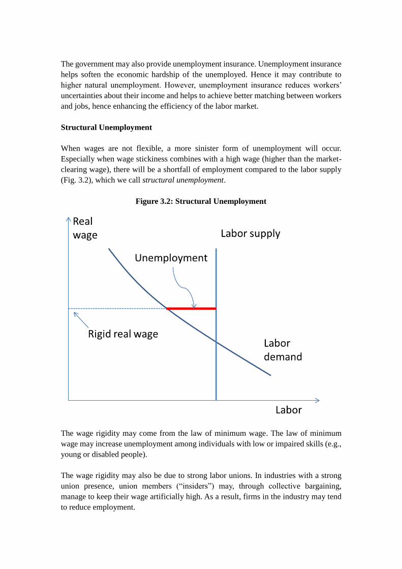
Structural Unemployment

When wages are not flexible, a more sinister form of unemployment will occur.

Especially when wage stickiness combines with a high wage (higher than the market-

clearing wage), there will be a shortfall of employment compared to the labor supply

(Fig. 3.2), which we call structural unemployment.

Figure 3.2: Structural Unemployment

The wage rigidity may come from the law of minimum wage. The law of minimum

wage may increase unemployment among individuals with low or impaired skills (e.g.,

young or disabled people).

The wage rigidity may also be due to strong labor unions. In industries with a strong

union presence, union members (“insiders”) may, through collective bargaining,

manage to keep their wage artificially high. As a result, firms in the industry may tend

to reduce employment.

The wage rigidity may also come from the practice of “efficiency wage.” Efficiency

wage refers to the practice to pay employees more than the market-equilibrium wage to

increase productivity or efficiency, or reduce costs associated with turnover. High wage

mitigates the problem of adverse selection since higher wage attracts and retains able

employees. High wage also mitigates the problem of moral hazards since high wage

increases the cost of possible job loss, the ultimate penalty of shirking. If a large number

of firms, however, resort to efficiency wage, then the overall wage level of the economy

would be higher than the market-clearing level, causing structural unemployment.

3.4 Income Distribution

As previously discussed, the total output and total income must equal the production

potential �̅�. The remaining question is how the income would be distributed among

owners of factor inputs, that is, those who provide capital and those who provide labor.

As we can imagine, factor prices (real wage and real rental price of capital) would be

crucial for the determination of the distribution. So the question hinges on the

determination of factor prices, which include real wage and real rental price of capital.

The real wage is the payment to labor measured in units of output, 𝑊

𝑃, where 𝑊 is

nominal wage and 𝑃 is the price of output. (In empirical studies, 𝑃 would be CPI or

GDP deflator).

Real rental price of capital is the rental price paid to the owner of capital in units of

output, 𝑅

𝑃, where 𝑅 is the nominal rent. In most cases, firm owners also own the capital

stock. But we can imagine that the firm rents capital from its owner and pays rent to the

owner of capital, just like the firm pays a wage to the owner of labor (i.e., workers).

A Representative Firm

We assume that the markets for goods and services are competitive and that the markets

for factors of production (labor and capital) are also competitive. Note that a market is

competitive if no participants are large enough to affect prices. In other words, all

market participants are price takers.

To determine the real wage and real rental price of capital, we look at the decision of a

“representative firm.” We may imagine that the economy is composed of many small

firms with the same technology 𝐹(𝐾𝑖, 𝐿𝑖), where 𝐾𝑖 and 𝐿𝑖 are capital and labor

inputs to the 𝑖-th firm, respectively. These firms produce the same product consumed

by consumers with the same taste (utility function). As a result, the total production of

the economy can be characterized by a representative firm with the production function

𝐹(𝐾, 𝐿), where 𝐾 and 𝐿 are total capital and labor of the economy, respectively. Here,

the constant-return-to-scale assumption on 𝐹 is crucial, making possible the

aggregation of firm-level technology into a macro production function.

The competitive firm takes as given the price of its output (𝑃), wage (𝑊), and real rental

price of capital (𝑅), and solves the following problem:

max𝐾,𝐿

𝑃 ⋅ 𝐹(𝐾, 𝐿) − 𝑊 ⋅ 𝐿 − 𝑅 ⋅ 𝐾.

That is, the firm tries to maximize economic profit.

Box 3.2 Economic Profit and Accounting Profit

Consider a firm with two factor-inputs: labor and capital. Economic profit is defined

as income (revenue) minus costs of labor and capital. And accounting profit is

defined by the sum of economic profit and the return to capital. Since most firms own

capital rather than rent them, return to capital is considered in accounting as profit.

The first-order condition for 𝐾 yields:

𝐹1(𝐾, 𝐿) = 𝑅/𝑃. (3)

where 𝐹1 ≡𝜕𝐹

𝜕𝐾 denotes the partial derivative of 𝐹 with respect to the first argument,

that is 𝐾. Equation (3) says that the firm would employ capital up to the point where

the marginal product of capital (MPK) equals the real rental price of capital.

And the first-order condition for 𝐿 yields:

𝐹2(𝐾, 𝐿) = 𝑊/𝑃. (4)

where 𝐹2 ≡𝜕𝐹

𝜕𝐿 denotes the partial derivative of 𝐹 with respect to the second

argument, that is 𝐿. Equation (4) says that the firm would employ labor up to the point

where the marginal product of labor (MPL) equals the real wage. Note that if we fix

𝐾 = �̅�, the first-order condition for 𝐿 gives us the demand curve for labor, i.e., the

relationship between real wage (𝑊

𝑃) and the labor demanded (𝐿): 𝐹2(�̅�, 𝐿) =

𝑊

𝑃. We

can check that, since we assume decreasing marginal product of labor, a lower real wage

corresponds to a higher demand for labor.

Income Distribution

Recall that the classical economy fully employs the total capital �̅�) and labor supply

(�̅�), which implies that �̅� and �̅� must solve Equation (1) and (2). That is to say, the

representative firm maximizes its profit when 𝐾 = �̅� and 𝐿 = �̅� . As a result, the

owner of labor receives 𝐹2(�̅�, �̅�) ⋅ �̅�, the owner of capital receives 𝐹1(�̅�, �̅�) ⋅ �̅�.

Interestingly, there is no economic profit (See Box 3.2) left for the whole economy. To

see this, note that under the constant-return-to-scale assumption on the production

function, we have 𝐹(𝑧𝐾, 𝑧𝐿) = 𝑧𝐹(𝐾, 𝐿) for any 𝑧 > 0. Then it follows

from 𝑑𝐹(𝑧𝐾,𝑧𝐿)

𝑑𝑧=

𝑑(𝑧𝐹(𝐾,𝐿))

𝑑𝑧 that

𝐹1(𝑧𝐾, 𝑧𝐿)𝐾 + 𝐹2(𝑧𝐾, 𝑧𝐿)𝐿 = 𝐹(𝐾, 𝐿).

Now let 𝑧 = 1 and use the fact that 𝐾 = �̅� and 𝐿 = �̅�, we have

𝐹1(�̅�, �̅�)�̅� + 𝐹2(�̅�, �̅�)�̅� = 𝐹(�̅�, �̅�) = �̅�.

Intuitively, recall the imagined economy with many small firms with the same

technology. Since the technology has constant return to scale, tiny would-be firms (say,

workshops) can enter the market and compete with existing ones. As a result, we may

deduce that there would be no “economic profit” for the existing firms.

Income Distribution in the Cobb-Douglas Economy

Suppose a classical economy is characterized by a Cobb-Douglas production function,

𝐹(𝐾, 𝐿) = 𝐸𝐾𝛼𝐿1−𝛼, we have

MPK = 𝐹1(𝐾, 𝐿) =𝛼𝐸𝐾𝛼𝐿1−𝛼

𝐾=

𝛼𝐹(𝐾, 𝐿)

𝐾

MPL = 𝐹2(𝐾, 𝐿) =(1 − 𝛼)𝐸𝐾𝛼𝐿1−𝛼

𝐿= (1 − 𝛼)

𝐹(𝐾, 𝐿)

𝐿

The capital’s share of income is

𝐹1(�̅�, �̅�) ⋅ �̅� = 𝛼𝐹(�̅�, �̅�) = 𝛼�̅�

The labor’s share of income is

𝐹2(�̅�, �̅�) ⋅ �̅� = (1 − 𝛼)𝐹(�̅�, �̅�) = (1 − 𝛼)�̅�

It would be an interesting empirical problem to check whether the shares of capital and

labor are indeed constants and how much. Fig. 3.3 shows, however, that the labor share

of income in China changes substantially over time. During the 1990s, the labor share

fluctuates around a level of around 67%. The labor share dropped substantially in the

first half of 2010s. The labor share reached the lowest point (58%) in 2008, after which

we see a strong rebound. In 2016, the labor’s share of income in China stood at 62%.

The United States has a much longer data set on the labor share of income. Fig. 3.4

shows the ratio of employee compensation in the national income. From 1929 to 1970,

we can see a secular upward trend. From 1970 to the early 1990s, the labor share

fluctuated around 66%. From the mid-1990s to 2014, we can see a secular downward

trend. It remains to be seen whether the 2014-bottom can hold for long term. Note that

we cannot directly compare the Chinese and the US share of labor income since the

methods of measurement are different.

Figure 3.3: Labor Share of Income in China

Figure 3.4: Labor Share of Income in the United States

Labor Productivity and Real Wage

Average labor productivity of an economy is defined by the average output, 𝑌

𝐿. In the

Cobb-Douglas economy, we have

MPL = 𝐹2(𝐾, 𝐿) = (1 − 𝛼)𝐸𝐾𝛼𝐿1−𝛼

𝐿= (1 − 𝛼)

𝑌

𝐿

Hence the MPL is proportional to average labor productivity in the Cobb-Douglas

economy. Once again, it would be interesting to investigate whether this is the case in

the real economy. Table 3.1 shows that, in the United States where long data is available,

the growth rates of labor productivity and real wage are positively correlated. At the

same time, however, the growth of real wage lags behind that of labor productivity. This

52

54

56

58

60

62

64

66

68

70

1992 1994 1996 1998 2000 2002 2004 2006 2008 2010 2012 2014 2016

50%

52%

54%

56%

58%

60%

62%

64%

66%

68%

19

29

19

33

19

37

19

41

19

45

19

49

19

53

19

57

19

61

19

65

19

69

19

73

19

77

19

81

19

85

19

89

19

93

19

97

20

01

20

05

20

09

20

13

20

17

observation is consistent with the fact that the labor’s share of income has been

declining in the US during the sample period.

Table 3.1: Growth in Labor Productivity and Real Wage in the US

Average Growth in Labor

Productivity (%)

Average Growth in Real

Nonfarm Compensation (%)

1959-2019 2.1 1.3

1959-1972 2.8 2.3

1973-1994 1.6 0.7

1995-2007 2.7 1.6

2008-2019 1.3 0.8

Data source: FRED.

3.5 Real Interest Rate, Consumption, and Investment

In this section, we present a classical macroeconomic model of the real interest rate.

The model specifies a set of behavioral assumptions and imposes an equilibrium

condition. We will use the model to examine the effects of external shocks (e.g., change

in fiscal policy) on a closed economy.

Let 𝑌 denote GDP. And recall that

𝑌 = 𝐶 + 𝐼 + 𝐺 + 𝑁𝑋, (5)

where 𝐶 represents consumption expenditure, 𝐼 represents investment expenditure,

𝐺 represents government expenditure, and 𝑁𝑋 represents net export. Equation (3)

was called the national income accounts identity in Chapter 2. However, we can also

interpret (3) as an equilibrium condition for an economy as a whole. For example, we

can interpret 𝑌 as the total supply in the market of goods and services, and the right-

hand-side of (3) represents the total demand. Then equation (3) states that, in

equilibrium, “supply must equal demand.” We will build a model on this equilibrium

condition.

In this section, we assume that there is no foreign trade. In other words, we consider a

closed economy with 𝑁𝑋 = 0. So we represent the equilibrium condition as

𝑌 = 𝐶 + 𝐼 + 𝐺.

In the following, we make a set of behavioral assumptions on the consumption

expenditure ( 𝐶 ) and investment expenditure ( 𝐼 ). Specifically, we introduce a

consumption function and an investment function to characterize consumption and

investment in the economy, respectively. And we regard the government expenditure

(𝐺) and tax (𝑇) as exogenous variables.

Consumption Function

Let 𝑇 denote the tax on households. The disposable income is then 𝑌 − 𝑇, the toal

income minus tax. The consumption function characterizes the total consumption

expenditure (𝐶) by a function of the disposable income, 𝐶(𝑌 − 𝑇). We assume that

𝐶(⋅) is an increasing function. That is, more disposable income leads to more

consumption.

On the consumption function, we may define the marginal propensity to consume (MPC)

as the amount of additional consumption given unit increase in disposable income.

Mathematically, MPC is clearly the first derivative of the consumption function with

respect to 𝑌,

𝑀𝑃𝐶 =𝑑𝐶(𝑌)

𝑑𝑌.

For example, if 𝐶(⋅) is a linear function, e.g.,

𝐶(𝑌 − 𝑇) = 100 + 0.7(𝑌 − 𝑇),

then MPC is a constant and MPC=0.7.

Real Interest Rate

We assume that the demand for investment goods depends on the interest rate, which

is the price of getting financing. Here we need to differentiate the real interest rate and

the nominal interest rate.

The real interest rate is the rate of interest a lender receives after allowing for inflation.

Unlike nominal interest rate, which we can directly observe in the market, the real

interest rate is not directly observable. However, we can calculate real interest rates

using the Fisher equation (named after Irving Fisher),

𝑟 = 𝑖 − 𝜋,

where 𝑖 is the nominal interest rate, 𝑟 is the real interest rate, and 𝜋 is the inflation

rate. For example: If the nominal interest rate is 5% and the inflation rate is 3%, then

the real interest rate is 2%. The real interest rate is the “real” return on deposit or the

“real” burden for a loan.

We may also use the modified Fisher equation,

𝑟 = 𝑖 − 𝐸𝜋,

where 𝐸𝜋 is the expectation of inflation. The real interest rate defined by the modified

is called the ex-ante real interest rate, 𝑟 = 𝑖 − 𝐸𝜋. The ex-ante real interest rate is

generally more reasonable than the ex-post real interest rate (𝑟 = 𝑖 − 𝜋) since when

loaners and debtors negotiate a (nominal) interest rate, they need to worry about the

inflation in the future.

Investment Function

Since higher real interest rate discourages borrowing and hence investment, we assume

that the investment expenditure of the economy is a decreasing function of the real

interest rate, 𝐼(𝑟) with 𝐼′(𝑟) < 0.

Fiscal Policy

The fiscal policy determines how much to tax and how much to spend by the

government. In this model, we capture the fiscal policy by two exogenous variables,

the tax revenue of the government (𝑇), and the government expenditure (𝐺). If 𝐺 = 𝑇,

we have a balanced budget; if 𝐺 > 𝑇, we have a budget deficit; and if 𝐺 < 𝑇, we have

a budget surplus.

When 𝐺 or 𝑇 changes, the private and public savings change. The private (non-

government) saving is defined by:

𝑆𝑛𝑔 = 𝑌 − 𝐶 − 𝑇.

And the public saving is defined by 𝑆𝑔 = 𝑇 − 𝐺. Adding 𝑆𝑔 and 𝑆𝑛𝑔 together, we

obtain national saving:

𝑆 = 𝑌 − 𝐶 − 𝐺.

Equilibrium in the Market for Goods and Services

In the market for goods and services, the demand side is characterized by

𝑌𝑑 = 𝐶(𝑌 − 𝑇) + 𝐼(𝑟) + 𝐺.

The supply side is

𝑌𝑠 = �̅�.

Recall that �̅� is the output potential of the economy. And, under the classical

assumptions, the AS curve is vertical and located at the output potential.

In the equilibrium of the market for goods and services, we must have demand equals

supply,

�̅� = 𝐶(�̅� − 𝑇) + 𝐼(𝑟) + 𝐺. (6)

In this model, the unknown real interest rate is the only endogenous variable. All the

remaining variables, 𝑇, 𝐺, and �̅�, are exogenous variables.

Equilibrium in the Financial Market

We may also interpret the equilibrium condition in (4) as an equilibrium in the financial

market.

We assume there exists a simple financial market for loanable funds. Those with

savings would lend their savings to borrowers (investors) in the financial market. The

national saving is 𝑌 − 𝐶 − 𝐺 , which is total income minus expenditures by the

households and the government. National saving is the supply of loanable funds in the

financial market. On the other hand, the demand for loanable funds comes from

investment need, 𝐼(𝑟).

In equilibrium, the real interest rate (𝑟) must adjust so that saving (supply of loanable

funds) equals investment (demand for loanable funds):

𝑆̅ ≡ �̅� − 𝐶(�̅� − �̅�) − �̅� = 𝐼(𝑟). (7)

Note that in the model, saving does not depend on the interest rate. The solution of the

above equilibrium equation is illustrated in Figure 3.5.

Figure 3.5: Determination of Real Interest Rate

The Effect of a Fiscal Stimulus

We may use our model to conduct a thought experiment on the effect of fiscal stimulus.

The fiscal stimulus may be in the form of increased government expenditure (increase

𝐺 ) or tax cut (decrease 𝑇 ), both of which would reduce national savings ( 𝑆 =

(�̅� − 𝐶(�̅� − 𝑇) − 𝐺)). An increase in 𝐺 would reduce national savings by reducing

public savings (𝑇 − 𝐺). A reduction of 𝑇 would reduce national savings by increasing

private consumption. The reduction of national savings shifts the saving curve (the

supply of loanable funds) to the left (Fig. 3.6), resulting in a higher equilibrium real

interest rate.

The model thus predicts that a fiscal stimulus would reduce national savings, resulting

in a higher interest rate and lower investment. Economists would say that such a

stimulus measure would “crowd out” the private investment. And under classical

assumptions, the crowding-out is complete, meaning that the stimulus fails to increase

total output or employment.

Figure 3.6: The Effect of Fiscal Stimulus

The Effect of Higher Investment Sentiment

For another example, we consider the case where there is a surge in investment

enthusiasm. That is, given any real interest rate, the investment demand for loanable

funds would increase. However, the national saving on the left-hand side of (7) does

not change. To make Equation (7) hold, the real interest rate has to increase. In the

meantime, the total investment does not change. Graphically, the downward sloping

demand curve shifts to the right. The equilibrium real interest rate increases and the

total investment remain unchanged. See Fig. 3.7.

Figure 3.7: Shifts in Investment Demand

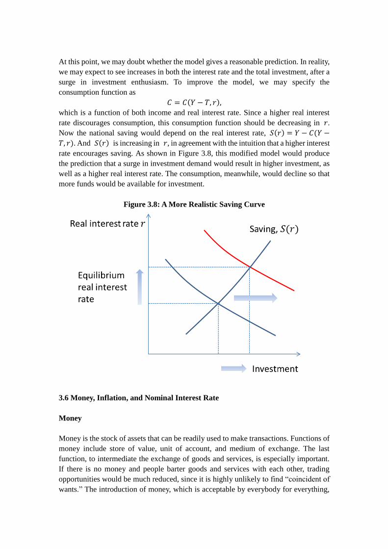
At this point, we may doubt whether the model gives a reasonable prediction. In reality,

we may expect to see increases in both the interest rate and the total investment, after a

surge in investment enthusiasm. To improve the model, we may specify the

consumption function as

𝐶 = 𝐶(𝑌 − 𝑇, 𝑟),

which is a function of both income and real interest rate. Since a higher real interest

rate discourages consumption, this consumption function should be decreasing in 𝑟.

Now the national saving would depend on the real interest rate, 𝑆(𝑟) = 𝑌 − 𝐶(𝑌 −

𝑇, 𝑟). And 𝑆(𝑟) is increasing in 𝑟, in agreement with the intuition that a higher interest

rate encourages saving. As shown in Figure 3.8, this modified model would produce

the prediction that a surge in investment demand would result in higher investment, as

well as a higher real interest rate. The consumption, meanwhile, would decline so that

more funds would be available for investment.

Figure 3.8: A More Realistic Saving Curve

3.6 Money, Inflation, and Nominal Interest Rate

Money

Money is the stock of assets that can be readily used to make transactions. Functions of

money include store of value, unit of account, and medium of exchange. The last

function, to intermediate the exchange of goods and services, is especially important.

If there is no money and people barter goods and services with each other, trading

opportunities would be much reduced, since it is highly unlikely to find “coincident of

wants.” The introduction of money, which is acceptable by everybody for everything,

solves this problem.

Furthermore, money makes pricing simple. Imagine a market with 𝑁 different goods,

but without money, we need 𝑁(𝑁 − 1)/2 pairs of price quotes. But if money is used

to intermediate exchanges, only 𝑁 price quotes are needed.

Given such convenience afforded by money, it is not surprising that human society uses

money, in one form or another, from very early history. At first, people use commodity

money (shells, gold, silver, etc.). But transactions using commodity money (say gold)

is costly since the purity and weight of a piece of gold have to be examined in every

transaction. To reduce transaction costs, a bank (possibly with authorization from the

government) may mint gold coins of known purity and weight. To further reduce cost,

the bank may issue gold certificates, which can be redeemed for gold. The gold

certificate eventually becomes gold-backed paper money.

In modern times, especially after the industrial revolution, economic growth speeds up.

The need for transactions grows faster than the growth of the gold supply. Hence the

limited supply of gold has a deflationary effect on the economy if countries stick to the

gold standard of money. Eventually, it is realized that if people do not care about the

option of redeeming gold, the bank can issue certificates that are not backed by gold in

the vault. The modern central bank does exactly this, and these certificates become fiat

money. Fiat money is valued because people expect it’s valued by everyone else.

Money in a modern economy may include cash, demand deposits, saving deposits,

money market funds, and so on. The supply of money is ultimately controlled by the

monetary authority (the central bank), which deliberate and implement monetary policy

to maintain low unemployment and moderate inflation. The monetary authority in

China is the People’s Bank of China (PBC). In the US, the monetary authority is the

Federal Reserve (the Fed).

Different types of money differ mainly in liquidity. Cash is the most liquid money while

saving deposits are much less liquid. The fact that there are different types of money

poses a problem for the measurement of the total money supply in the economy. We

usually use several measures (M0, M1, M2, etc.), classified along a spectrum between

the narrowest and the broadest measurements. Narrow measures include the most liquid

types of money, while broad measures include illiquid money. In China, M0 includes

only cash in circulation, M1 includes demand deposits in addition to M0, and M2 is

roughly M1 plus saving deposits. In 2015, M0, M1, and M2 were 6.3, 40.1, 139.2

trillion Yuan, respectively.

Inflation, Deflation, and Disinflation

Inflation is a sustained increase in the general price level of goods and services.

Temporary fluctuations in price level do not constitute inflation. For example, seasonal

increase in price before and during the Spring Festival in China may not be inflation,

since the price would often decline after the holiday, as demand wanes and supply

recovers. Price increases in some particular goods or services are also not regarded as

inflation unless they are accompanied by the rise in the general price level.

If there is a sustained decrease in the general price level, we call it deflation. A related

concept is disinflation, which refers to the case where the inflation rate declines. As

discussed in the previous chapter, we use CPI or GDP deflator to measure inflation.

When there is inflation, the purchasing power of the money declines. And there are

losers and winners from inflation. Losers include people who save, people who hold

bonds, and, generally, people who receive fixed incomes. The retired pensioners are

especially vulnerable. Unexpected inflation is equivalent to redistribution of wealth

from savers to borrowers, who are winners of inflation. Unexpected inflation also

increases a sense of uncertainty in the economy, discouraging investment.

Even expected inflation has costs. First, high inflation leads to a high frequency of price

changes, which are costly because sellers and buyers have to renegotiate prices, and

new menus have to be printed (metaphorically, menu costs). Second, high inflation

leads to high opportunity cost in holding cash, causing inconveniences of insufficient

cash holding. It can be metaphorically called “shoe-leather cost,” meaning that more

frequent visits to banks would cause one’s shoes to wear out more quickly. Third, high

inflation makes price signal noisy, affecting the ability of the “invisible hand” to

allocate resources. Fourth, tax brackets are often in nominal terms (e.g., the minimum

taxable monthly salary is 3500 Yuan in China), high inflation would make tax burden

heavier than is intended to.

When prices lose control and inflation skyrockets, the economy may fall into a full

crisis. According to a loose definition, if inflation exceeds 50% per month, we call the

phenomenon hyperinflation. All the costs of moderate inflation described above

become prohibitive under hyperinflation. Money ceases to function as a store of value,

and may not serve its other functions (unit of account, medium of exchange). People

may have to barter or use a stable foreign currency.

What causes hyperinflation? An easy answer is that hyperinflation is caused by

excessive money supply growth. When the central bank prints money, the price level

rises. If it prints money rapidly enough, the result is hyperinflation. But why would a

central bank print money like crazy? In most cases, it would be due to fiscal problems.

When a government experiences fiscal crisis due to either extraordinary expenditure

(war, indemnity, etc.) or impaired tax power or both, the government may resort to

excessive money printing.

These said, there is one benefit of moderate inflation, which proves important for the

health of macroeconomy. It is a fact that nominal wages are rarely reduced, even when

the equilibrium real wage falls during recessions. Inflation allows real wages to reach

equilibrium levels without cutting the nominal wage. Therefore, moderate inflation

improves the functioning of labor markets.

On the other hand, deflation may look good, since it implies increased purchasing

power of money. But deflation is almost intolerable in a modern economy, as it makes

debts more difficult to service, discourages investment, and thus aggravates

unemployment problem. This is why, recently, central banks around the world have

been conducting aggressive monetary policies (quantitative easing, negative interest

rates, etc.) to maintain positive inflation.

Quantity Theory of Money

The quantity theory of money is the centerpiece of what classical theory has to say

about money and inflation.

Let 𝑇 be the total number of transactions during a period, 𝑃 the overall price, and 𝑀

the money in circulation. We may define the transaction velocity of money by

𝑉 ≡𝑃𝑇

𝑀.

The quantity theory of money is thus stated as an identity,

𝑀𝑉 = 𝑃𝑇.

The number of transactions is difficult to measure, even in a small economy. But it is

intuitively clear that the number of transactions is closely related to the total real income

of the economy since each transaction brings income to the parties involved.

If we proxy the total transactions by the total real income (e.g., real GDP), we obtain a

more practical quantity theory of money:

𝑀𝑉 = 𝑃𝑌, (8) ⑶

where 𝑌 denotes total income (e.g., real GDP). Note that the new version of quantity

theory is nothing but an alternative definition of the velocity of money.

We may also interpret the equation in (3) as an equilibrium condition in the money

market. Rewrite (8) as

𝑀/𝑃 = 𝑘𝑌, (9) ⑶

where 𝑘 ≡ 1/𝑉. If 𝑉 is, as usual, assumed to be a constant, so is 𝑘. We may interpret

the left-hand side as the real money supply and the right-hand side as money demand,

which is assumed to depend on the total income only. The equilibrium condition is thus,

“real money supply” = “money demand.”

𝑘 characterizes how much money people wish to hold for each unit of income. It is by

definition inversely proportional to 𝑉: when people hold lots of money relative to their

incomes, money changes hands infrequently.

Money and Inflation

From the quantity theory of money, we can obtain

𝑑𝑀

𝑀+

𝑑𝑉

𝑉=

𝑑𝑃

𝑃+

𝑑𝑌

𝑌.

Note that 𝑑𝑀

𝑀 and

𝑑𝑌

𝑌 are growth rates of money supply and real GDP, respectively,

and that 𝑑𝑃

𝑃 is the inflation rate. If we assume that the velocity 𝑉 is constant, then

𝑑𝑉

𝑉= 0. The quantity theory of money implies that, given the real GDP growth rate, a

higher growth rate of the money supply leads to higher inflation.

In the real world, inflation does not necessarily co-move with the growth in the money

supply (Fig. 3.9). However, if we take a long-term view, say examine the 30-year

inflation and growth in the money supply in cross-country data, we can observe a

significant positive correlation between the two.

Figure 3.9: Inflation and Money Growth in China

Inflation and Nominal Interest Rate

Recall that, in the classical model of the real interest rate, the real interest rate is

determined in the market for loanable funds, 𝐼(𝑟) = 𝑌 − 𝐶 − 𝐺. If the real variables

(𝑌, 𝐶, 𝐺 ) are given, so is 𝑟 . Then the nominal interest rate, according to Fisher’s

equation, has a one-to-one relationship with the inflation rate (Fisher effect),

𝑖 = 𝑟 + 𝜋. (10)

-5.0

0.0

5.0

10.0

15.0

20.0

25.0

30.0

35.0

40.0

Inflation M2 Growth

For example, in a static economy (𝑌 = �̅�), a 1% increase in the growth rate of the

money supply would cause a 1% increase in inflation rate and then a 1% increase in the

nominal interest rate.

Classical Dichotomy

We can combine the classical AD-AS model in (1), the classical model of real interest

rate in (6), the quantity theory of money in (9), and the Fisher equation in (10),

𝑌 = �̅�

𝑌 = 𝐶(𝑌 − 𝑇) + 𝐼(𝑟) + 𝐺,

𝑀

𝑃= 𝑘𝑌,

𝑖 = 𝑟 + 𝜋.

Note that in this integrated model, real variables (e.g., 𝑌 and 𝑟 ) are determined

without considering money. Money supply only influences the general price level,

which in turn determines the nominal values such as nominal GDP, nominal interest

rate (𝑖), and so on. The idea of separating “real” from “nominal” analysis is called the

classical dichotomy. If the classical dichotomy holds, we also say that money is neutral.

Naturally, monetary policy is irrelevant if money is indeed neutral. The expansion of

the money supply, according to the classical theory, only drives up the price level and

does not influence the output or employment, both of which are “real” variables. In the

real world, however, evidence abounds that monetary policy has real effects on output

or employment.

To Improve the Quantity Theory of Money

As we have seen earlier, the quantity theory of money gives a poor prediction about the

short-term relationships between money and inflation. We may suspect that the simple

model of money demand ((𝑀

𝑃)

𝑑

= 𝑘𝑌) is not realistic. Money demand may well depend

on other factors than the total income 𝑌. For example, variables like interest rates,

consumer and investor confidence, debt level, etc., may also significantly influence

money demand. Indeed, money velocity is highly unstable in history (Fig. 3.10).

To improve the quantity theory of money, we may write the money demand function as

(𝑀

𝑃)

𝑑

= 𝐿(𝑖, 𝑌),

where 𝑖 is the nominal interest rate. The nominal interest rate 𝑖 is the opportunity cost

of holding money (instead of bonds or other interest-earning assets). Hence, an increase

in 𝑖 lowers the money demand and the function 𝐿(𝑖, 𝑌) would be decreasing in 𝑖 and

increasing in 𝑌. (𝐿 is used to denote the money demand function because money is the

most liquid asset.)

Equate demand to supply, we obtain

𝑀

𝑃= 𝐿(𝑖, 𝑌) = 𝐿(𝑟 + 𝐸𝜋, 𝑌),

This equilibrium condition establishes a relationship between inflation and the real

money supply (𝑀/𝑃). In this case, the money velocity would be given by

𝑉 ≡𝑃𝑌

𝑀=

𝑌

𝐿(𝑟 + 𝐸𝜋, 𝑌),

which allows more volatility.

Figure 3.10: Money Velocity (Nominal GDP/M2)

3.7 Exchange Rate

In the section, we consider the open economy that trades with other economies in the

world. We first study the international flows of goods and capital in national accounting.

We then introduce the exchange rate, which is the most important variable in the

discussion of open economy. Next we study a model of small open economy and a

model of large open economy. Small and large economies differ in whether their saving

and investment may affect the world interest rate.

In an open economy, domestic spending need not equal its output. The difference is the

net export, which is the total value of export minus that of import. In short,

𝑌 − (𝐶 + 𝐼 + 𝐺) = 𝑁𝑋 = 𝐸𝑋 − 𝐼𝑀,

where 𝑌 is output, (𝐶 + 𝐼 + 𝐺) represents domestic spending, 𝑁𝑋 stands for net

export, 𝐸𝑋 stands for export, and 𝐼𝑀 stands for import. All these variables are in the

“real” sense.

If the domestic spending is less than the output, then 𝑁𝑋 > 0 and the surplus is lent

to foreigners. If the domestic spending exceeds the output, then 𝑁𝑋 < 0 and the

0

0.2

0.4

0.6

0.8

1

1.2

1.4

19

90

19

91

19

92

19

93

19

94

19

95

19

96

19

97

19

98

19

99

20

00

20

01

20

02

20

03

20

04

20

05

20

06

20

07

20

08

20

09

20

10

20

11

20

12

20

13

20

14

20

15

20

16

20

17

20

18

country borrows (−𝑁𝑋) from abroad. The net export is also called the trade balance.

The flow of goods and services is mirrored by capital flow. Let 𝑆 = 𝑌 − (𝐶 + 𝐺) be

the national saving. By the national income accounting identity, we have

𝑆 − 𝐼 = 𝑁𝑋.

We may call (𝑆 − 𝐼) the net capital outflow (𝐶𝐹). The above equation says that the

net capital outflow always equals the net export, 𝐶𝐹 = 𝑁𝑋.

• If 𝑆 − 𝐼 = 𝑁𝑋 > 0, the country lends its surplus saving (𝑆 − 𝐼) to foreigners.

• If 𝑆 − 𝐼 = 𝑁𝑋 < 0, then the country borrows (−𝑁𝑋), the saving deficit, from

abroad.

To understand this identity more intuitively, we examine an imagined example. If BYD

sells an electric car to a US consumer for $10,000, how does the sale change China’s

trade and capital flow? On trade, The Chinese export rises by $10,000. On capital flow,

if BYD invests the $10,000 in the US securities (e.g., stocks or bonds), then Chinese

capital outflow rises by $10,000. The same is true even if BYD keeps the cash. If BYD

converts the $10,000 into RMB at a local Chinese bank, then the bank also has to do

something about it. If the bank chooses to purchase the US securities or to keep the

dollar cash, then Chinese capital outflow again rises by $10,000. If the bank sells the

dollar to PBC and PBC uses the $10,000 to purchase US treasury bills, we still see a

$10,000 rise in capital outflow.

3.7.1 Exchange Rate

The exchange rate (also known as the foreign-exchange rate, or forex rate) between two

currencies is the rate at which one currency exchanges for another.

We may express the exchange rate in units of foreign currency per the domestic

currency. For example, the exchange rate of Korean Won is typically quoted in the unit

of Won/Yuan. The exchange rate may also be in units of domestic currency per foreign

currency. For example, the exchange rate of USD is typically quoted in the unit of

Yuan/USD.

In this course, we adopt the convention that the exchange rate is in units of foreign

currency per the domestic currency (Yuan). Under this convention, a rise in the

exchange rate is called appreciation of RMB; a fall in the exchange rate is called

depreciation. Appreciation is also called strengthening, while depreciation is also called

weakening.

The real exchange rate is the purchasing power of a currency relative to another

currency at current nominal exchange rates and prices. Let 𝑒 be the nominal exchange

rate, 𝑃 the domestic price level, 𝑃∗ the foreign price level. Then the real exchange

rate is defined by

𝜀 =

𝑒𝑃

𝑃∗. (11)

It is obvious that the lower the real exchange rate, the less expensive are domestic goods

and services relative to foreign ones.

Because a country trades with many countries, it is often useful to calculate the effective

exchange rate, an index measuring the weighted average appreciation of a currency

against a basket of foreign currencies. The nominal effective exchange rate is calculated

with nominal exchange rates. The real effective exchange rate is calculated with real

exchange rates.

Graph: (1) RMB/USD Exchange Rate; (2) RMB Effective Exchange Rates

It is interesting to note that during 2015, the Chinese RMB depreciated about 8%

against the US dollar. But in terms of effective exchange rates, RMB appreciated

approximately 10% relative to its trading partners. So looking at one particular bilateral

exchange rate, however important it is, can miss the big picture of a currency’s

exchange rate movement.

3.7.2 Purchasing Power Parity (PPP)

Examining the definition of the real exchange rate in (11), we can see that if domestic

and foreign currencies have identical purchasing power, then the real exchange rate (𝜀)

should be exactly one. Indeed, if 𝜀 = 1 , we say that the exchange rates are at

purchasing power parity. Theoretically, PPP is implied by “the law of one price.” If

𝜀 > 1, the domestic currency is overvalued in terms of purchasing power. If 𝜀 < 1, the

domestic currency is under-valued in terms of purchasing power.

For example, suppose both China and the USA produce and consume one good, the Big

Mac. The Big Mac costs 20 Yuan in China and 4 USD in the USA. The nominal

exchange rate is 6 RMB/USD. Then the real exchange rate between China and USA is

1

6⋅

20

4=

5

6. Since the real exchange rate is less than 1, we say that PPP does not hold,

and RMB is undervalued: One Chinese Big Mac costs 5/6 of what an American Big

Mac costs.

If PPP holds, we have

𝑒𝑡 =𝑃𝑡

∗

𝑃𝑡.

Taking log difference (log(𝑒𝑡) − log (𝑒𝑡−1)), we have

Δ𝑒𝑡

𝑒𝑡−1= 𝜋𝑡

∗ − 𝜋𝑡 , (12)

where 𝜋𝑡∗ and 𝜋𝑡 are foreign and domestic inflations, respectively. In particular, note

that 𝜋𝑡 = log (𝑃𝑡/𝑃𝑡−1). This is to say, PPP implies that if foreign inflation is higher

than domestic inflation, the domestic currency would appreciate by the inflation gap

(𝜋𝑡∗ − 𝜋𝑡).

If we further assume a common real interest rate, then we have

Δ𝑒𝑡

𝑒𝑡−1= 𝑖𝑡

∗ − 𝑖𝑡. (13)

where 𝑖𝑡∗ and 𝑖𝑡 are foreign and domestic nominal interest rates, respectively. The

above equation says that if the foreign nominal interest rate is higher than the domestic

one, the domestic currency tends to appreciate. The equation in (13) is often called

“uncovered interest rate parity,” which characterizes an equilibrium where investors of

the weak currency have to be compensated with a higher interest rate.

PPP must hold if the “law of one price” applies. However, PPP may not hold, especially

in the short term. First, not all goods are tradable. Second, there are trading barriers and

trading costs. These make cross-country arbitrage of price differences incomplete and

costly. As a result, researchers find little empirical support for PPP if they use short-

term data to test implications of PPP, say Equation (12). If they use long-term data, say

10-year inflation differentials between countries and percentage changes in exchange

rates, they would find more support of PPP.

3.7.3 A Model of Small Open Economy

Now we introduce an open-economy model that characterizes the determination of the

real exchange rate, which further determines net export or net capital outflow. We build

the model on the same equilibrium condition in (5). However, we shall give it a new

interpretation. Equation (5) implies that

𝑆 − 𝐼 = 𝑁𝑋, (14)

where 𝑆 = 𝑌 − 𝐶 − 𝐺 , and (𝑆 − 𝐼) represents the excess (national) saving. The

excess saving has to flow out of the country and equals the net capital outflow. Let 𝐶𝐹

denote net capital outflow; we have 𝐶𝐹 = 𝑆 − 𝐼 . We may interpret the net capital

outflow, the left-hand-side of (14), as the demand for foreign currency. The net export,

on the other hand, represents the supply of foreign currency. Then we may interpret (14)

as an equilibrium condition on the foreign exchange market, where exporters would sell

their foreign currency to those who want to hold foreign assets.

To finish building the model, we now impose some behavioral assumptions on 𝐼 and

𝑁𝑋 . Note that the national saving 𝑆 = 𝑌 − 𝐶 − 𝐺 is exogenous since, under the

classical assumptions, the output 𝑌 equals the potential output �̅�, and that 𝐶 is a

function of (�̅� − 𝑇), also an exogenous variable.

Recall that in Section 3.5, we assume that the investment expenditure is a decreasing

function of the real interest rate, 𝐼(𝑟). Here, we retain this assumption but note that the

real interest rate in the small open economy would be equal to the real interest rate

prevailing in the world, 𝑟 = 𝑟∗. To justify this, we may assume that capital is perfectly

mobile across borders. As a result, global arbitragers would make sure the real interest

rate is the same across the world.

We also assume that 𝑟∗ is exogenous, meaning that it is determined outside the model.

To justify this, we assume that the excess saving of the small economy does not affect

the world interest rate. In other words, the small economy is a “price taker” of the world

interest rate 𝑟∗.

On the net export 𝑁𝑋 , we assume that 𝑁𝑋 is a decreasing function of the real

exchange rate (𝜀), 𝑁𝑋(𝜀) with 𝑁𝑋′(𝜀) < 0. This is a reasonable assumption since a

higher real exchange rate encourages imports and makes the export sector less

competitive.

Now we re-write the equilibrium condition in (14) as

𝑆 − 𝐼(𝑟∗) = 𝑁𝑋(𝜀), (15)

where 𝑆 = (�̅� − 𝐶(�̅� − 𝑇) − 𝐺). Since 𝑆 and 𝑟∗ are exogenous, the demand side of

the foreign exchange market (the left-hand side of (15)) is given. The equilibrium real

exchange rate adjusts the right-hand side to make supply equal to demand. Figure 3.11

illustrates the solution of the model graphically.

Figure 3.11: The Equilibrium of the Foreign Exchange Market

Next, we may conduct thought experiments on the above small open economy model.

We may analyze the effects of the following changes: a fiscal stimulus, a rise in the

world interest rate, and an implementation of protectionist trade policy.

Fiscal Stimulus

We know that a fiscal stimulus reduces national saving, thus reducing the excess saving

(𝑆 − 𝐼, demand for foreign currency). The reduction of national savings would shift the

excess-saving curve (Fig. 3.11) to the left, resulting in a higher equilibrium real

exchange rate. That is, the domestic currency would appreciate, depressing export. As

the total output remains at the level of potential output, the reduction of export must be

such that the fiscal stimulus would fail to stimulate the total output or employment. This

prediction is similar to the complete “crowding-out” of the investment by a fiscal

stimulus in the closed economy.

A Rise in the World Interest Rate

If the world interest rate rises, the investment expenditure will decline. As a result, the

excess savings (𝑆 − 𝐼) will increase, shifting the excess-saving curve (Fig. 3.11) to the

right. The equilibrium real exchange rate will decline, stimulating the net export. As

always, under the classical assumptions, the total output remains at the potential level.

When a rising world interest rate depresses the investment demand, a rising foreign

demand fully compensates for the loss of aggregate demand due to the depreciation of

the exchange rate.

Protectionist Policy Shock

Suppose that the government implements a protectionist policy that discourages import

and encourages export. At every real exchange rate (𝜀), the policy would make the net

export 𝑁𝑋(𝜀) bigger. As a result, the 𝑁𝑋 curve would shift to the right, and the

equilibrium real exchange rate will rise. Thus the classical model predicts that the

protectionist policy would fail to lift the net export. The only effect of the policy is the

appreciation of the domestic currency.

The reason why we reach such a dramatic conclusion is that we assume the excess

savings (𝑆 − 𝐼) does not depend on the exchange rate. And the excess savings alone

determine the net export in our model. To increase net export or decrease the trade

deficit, the classical economists would argue, the government should increase national

savings by, for example, cutting government expenditure.

3.7.4 A Model of Large Open Economy

In the small open economy model, we assume that the economy is a “price taker” of

the world interest rate 𝑟∗. That is, the excess saving of the economy does not affect the

world interest rate. If this condition does not hold, meaning that the capital outflow of

the economy does affect the world interest rate, then we have to develop a model with

two endogenous variables, the world (real) interest rate 𝑟 and the real exchange rate

(𝜀). We call it a model of large open economy. Presumably, the savings and investment

behavior of a large economy would have an impact on the world interest rate.

We make the following assumptions:

(i) Capital is perfectly mobile across borders.

(ii) The net export is a decreasing function of the real exchange rate (𝜀).

(iii) The net capital outflow of the large economy (𝐹) is a decreasing function of the

world interest rate 𝑟, 𝐹(𝑟) with 𝐹′(𝑟) < 0.

The first two assumptions are the same as in the small open economy model. The third

assumption defines To see why it is reasonable to assume that 𝐹(𝑟) is decreasing, note

that the net capital outflow of a large economy would depress the world interest rate.

In this model, there are two markets, one for loanable funds, the other for foreign

exchange. In equilibrium, we have

𝑆 = 𝐼(𝑟) + 𝐹(𝑟), (16)

𝑁𝑋(𝜀) = 𝐹(𝑟). (17)

We have two endogenous variables in the model of two equations: the world real

interest rate (𝑟) and the real exchange rate (𝜀). The analysis of the model, however, is

straightforward. Note that there is only one endogenous variable (𝑟) in (16), which

solely determines the equilibrium real interest rate 𝑟∗ . Next, we can analyze the

equilibrium exchange rate 𝜀, treating 𝑟∗ as given.

Graphically, Equation (16) corresponds to the vertical line on the two-dimensional

diagram in Fig. 3.12. On the other hand, Equation (17) dictates that a bigger 𝑟 must

accompany a bigger 𝜀. Thus the curve corresponding to Equation (17) must be upward-

sloping.

Figure 3.12: The Model of Large Open Economy

Using the model, we can conduct thought experiments on a large open economy. We

first analyze the impact of a fiscal stimulus on the economy. Then we analyze what

would happen if the government implements a protectionist policy.

Fiscal Stimulus

The fiscal stimulus, whether in the form of increased government expenditure or tax

reduction, is a negative shock to the national savings (𝑆). We first analyze the impact

of the shock on the equilibrium interest rate 𝑟∗ by inspecting (16). Then we analyze

the impact on 𝜀∗, treating the change in 𝑟∗ as given.

Since both 𝐼(𝑟) and 𝐹(𝑟) are decreasing functions of 𝑟 , 𝑟∗ must rise when 𝑆

declines. Graphically, the vertical line in Fig. 3.12 shifts to the right. As a result, the

equilibrium exchange rate also rises.

We may verify the second prediction by inspecting (17). Since 𝐹(𝑟∗) has declined

after the negative shock to 𝑆 , 𝑁𝑋(𝜀∗) should also decline. Since 𝑁𝑋(𝜀) is

decreasing in 𝜀 , the equilibrium exchange rate 𝜀∗ must rise (appreciate). In

conclusion, a negative shock to national saving would result in a higher real interest

rate and an appreciation of the domestic currency.

Protectionist Shock

A protectionist policy shock may be in the form of raising tariffs on imported goods or

boycotting some foreign goods. The protectionist shock would have an impact on the

net export function 𝑁𝑋(⋅). We now analyze how the upward-sloping curve (𝑁𝑋(𝜀) =

𝐹(𝑟)) shifts under the shock.

As the shock happens, given any 𝜀, 𝑁𝑋(𝜀) would increase. To make 𝐹(𝑟) increase

as well, 𝑟 must decline. As this is true for every 𝜀 , we conclude that the curve

(𝑁𝑋(𝜀) = 𝐹(𝑟)) must shift to the left.

Hence a protectionist shock (e.g., raising import tariffs) would result in the appreciation

of the domestic currency. This prediction is consistent with that of the small open

economy.

Exercises:

1. Suppose that the output of an economy can be characterized by the Cobb-Douglas

function,

𝐹(𝐾, 𝐿) = 𝐸𝐾𝛼𝐿1−𝛼, 0 < 𝛼 < 1.

(1) Calculate the marginal product of labor (MPL) and the marginal product of capital

(MPK). Check whether they are positive.

(2) Calculate the second derivatives. Check that MPL is decreasing as 𝐿 increases and

that MPK is decreasing as 𝐾 increases.

(3) Verify that the Cobb-Douglas function satisfies constant-return-to-scale.

2. Suppose that every year in Shanghai, 2% of married couples get divorced and 3%

of single adults get married. In the steady state, what is the percentage of married

people in the adult population?

3. Suppose that an economy has two sectors: manufacturing and services. The labor

demand curve in these two sectors are different as follows,

𝐿𝑚 = 200 − 6𝑊𝑚

𝐿𝑠 = 100 − 4𝑊𝑠

where 𝐿 and 𝑊 denote labor (number of workers) and wage, respectively, and

the subscripts denote the sectors. The economy has a labor force of 100.

(1) If workers are free to move between sectors and there is no skill barrier, then

calculate wage and employment in each sector.

(2) Now suppose that the manufacturing union manages to raise the wage in the

manufacturing sector to 25 and that all workers who cannot get manufacturing

jobs move to the service sector. Calculate the wage and employment in each

sector.

(3) Now suppose that all workers have a reservation wage of 15. We may assume

that a worker with a wage below 15 cannot afford to live in the city. He would

rather go back to the countryside, where living cost is minimal, to wait for a

union job (with wage 25) to open up. What is the economy’s unemployment

rate?

4. Apply the classical theory of income distribution to predict the effect on the real

wage and the real rental price of capital if the following events happen:

(1) An earthquake damages part of the capital stock.

(2) The government raises the retirement age.

(3) Inflation raises all prices (output price and factor-input prices) by 10%.

(4) A technological breakthrough improves the production function (suppose the

production function is labor-augmenting).

(5) Following (4), what if the production function is capital-augmenting.

5. Consider a closed economy characterized by the following equilibrium condition

and specifications:

Y = C(Y − T) + I(r) + G,

Y = 8000, G = 1000, T = 800,

C(Y − T) = 1000 +3

4(𝑌 − 𝑇),

I(r) = 1200 − 100r.

(1) Calculate private saving, public saving, and national saving.

(2) Calculate the equilibrium real interest rate.

(3) Suppose that the government reduces its expenditure to achieve a balanced

budget. Calculate private saving, public saving, and national saving. And

calculate the new equilibrium real interest rate.

6. The following table lists some exchange rates and Big-Mac prices. Use the theory

of purchasing-power parity to fill in the blanks with a number or “?” if the figure

cannot be inferred from the information.

Country Currency Big-Mac

price

Exchange rate (per US dollar)

Predicted

(PPP)

Actual

USA Dollar 4.8

China Yuan 18 7

Japan Yen 75 100

UK Pound 3.6 0.75

7. Consider a small open economy characterized by the following equilibrium

condition and specifications:

Y = C(Y − T) + I(r) + G + NX(ε),

Y = 8000, G = 1000, T = 800,

C(Y − T) = 1000 +3

4(𝑌 − 𝑇),

I(r) = 1200 − 100r,

NX(ε) = 500 − 200ε,

r = r∗ = 5.

(1) Calculate the national savings, excess savings, and net capital outflow.

(2) Calculate the equilibrium real exchange rate.

(3) Suppose that the government increases its expenditure by 200 and leave tax

unchanged (in effect, the budget deficit increases by 200.). Calculate the private

savings, the national savings, the excess savings, and the net capital outflow.

And calculate the new equilibrium real exchange rate.

8. Consider a large open economy with flexible prices. What would happen to the

interest rate and exchange rate, if the following events occur?

(1) A business-friendly party wins the election and takes control of the government.

(2) In the name of “national security,” the government increases tariffs on goods

from a major trading partner.

(3) After a terrorist attack, the country goes to war in the Middle East.