chapter 3 calculating the wqcv and volume reduction · calculating the wqcv and volume reduction...
TRANSCRIPT
August 2011 Urban Drainage and Flood Control District 3-i
Urban Storm Drainage Criteria Manual Volume 3
Chapter 3 Calculating the WQCV and Volume Reduction Contents 1.0 Introduction ...................................................................................................................................... 1
2.0 Hydrologic Basis of the WQCV ...................................................................................................... 1 2.1 Development of the WQCV ...................................................................................................................... 1 2.2 Optimizing the Capture Volume ............................................................................................................... 3 2.3 Attenuation of the WQCV (BMP Drain Time) ......................................................................................... 4 2.4 Excess Urban Runoff Volume (EURV) and Full Spectrum Detention ..................................................... 4
3.0 Calculation of the WQCV ................................................................................................................ 5
4.0 Quantifying Volume Reduction .................................................................................................... 10 4.1 Conceptual Model for Volume Reduction BMPs—Cascading Planes .................................................... 10 4.2 Watershed/Master Planning-level Volume Reduction Method ............................................................... 11 4.3 Site-level Volume Reduction Methods ................................................................................................... 14
4.3.1 SWMM Modeling Using Cascading Planes ................................................................................ 15 4.3.2 IRF Charts and Spreadsheet ........................................................................................................ 16
4.4 Other Types of Credits for Volume Reduction BMPs/LID ..................................................................... 20
5.0 Examples ......................................................................................................................................... 21 5.1 Calculation of WQCV ............................................................................................................................. 21 5.2 Volume Reduction Calculations for Storage-based Approach ................................................................ 22 5.3 Effective Imperviousness Spreadsheet .................................................................................................... 23
6.0 Conclusion ....................................................................................................................................... 34
7.0 References ....................................................................................................................................... 35
Figures Figure 3-1. Map of the Average Runoff Producing Storm's Precipitation Depth in the United States ....... 3Figure 3-2. Water Quality Capture Volume (WQCV) Based on BMP Drain Time .................................... 6Figure 3-3. Watershed Imperviousness, Single Family Residential Ranch Style Houses ........................... 7Figure 3-4. Watershed Imperviousness, Single Family Residential Split-Level Houses ............................ 8Figure 3-5. Watershed Imperviousness, Single Family Residential Two-Story Houses ............................. 9Figure 3-6. Four Component Land Use ..................................................................................................... 11Figure 3-7. Effective Imperviousness Adjustments for Level 1 MDCIA .................................................. 13Figure 3-8. Effective Imperviousness Adjustments for Level 2 MDCIA .................................................. 14Figure 3-9. Conveyance-based Imperviousness Reduction Factor ............................................................ 18Figure 3-10. Storage-based Imperviousness Reduction Factor ................................................................. 19Figure 3-11. Colorado Green Development DCIA, UIA, RPA, and SPA ................................................. 31Figure 3-12. Colorado Green Precipitation Input Screen Shot .................................................................. 32Figure 3-13. Colorado Green Area and Infiltration Input Screen Shot ...................................................... 32Figure 3-14. Colorado Green Calculated Output Screen Shot ................................................................... 32
3-ii Urban Drainage and Flood Control District August 2011
Urban Storm Drainage Criteria Manual Volume 3
Figure 3-15. Colorado Green Imperviousness Reduction Factor Volume-based Lookup ......................... 33Figure 3-16. Colorado Green IRF Conveyance-based Lookup .................................................................. 34
Tables Table 3-1. Number of Rainfall Events in the Denver Area .......................................................................... 2Table 3-2. Drain Time Coefficients for WQCV Calculations ...................................................................... 5Table 3-3. Infiltration Rates (f) for IRF Calculations ................................................................................. 17

Chapter 3 Calculating the WQCV and Volume Reduction
August 2011 Urban Drainage and Flood Control District 3-1 Urban Storm Drainage Criteria Manual Volume 3
Using WQCV and Flood Control Hydrology
Channels are typically designed for an event that is large and infrequent, such as the 100-year event. A common misconception is that these large events are also responsible for most of the erosion within the drainageway. Instead, the effective discharge, by definition, is the discharge that transports the most bedload on an annual basis and this is, therefore, a good estimate of the channel-forming flow or the discharge that shapes the drainageway through sediment transport and erosion. The effective discharge does not correlate with a specific return period, but typically is characterized as a magnitude between the annual event and the 5-year peak, depending on reach-specific characteristics.
The typical flood control facility design may include peak reduction of the 5- or 10-year storm event as well as the 100-year event. Widespread use of this practice reduces flooding of streets and flooding along major drainageways. However, this practice does little to limit the frequency of channel-forming flows in drainageways. UDFCD recommends Full Spectrum Detention, a concept developed to replicate historic peak flows more closely for a broad spectrum of storm events. Widespread use of Full Spectrum Detention would, in theory, improve channel stability and reduce erosion; however, implementation of Full Spectrum Detention may not be feasible on all sites. Therefore, this manual provides a variety of storage-based BMPs that provide the WQCV and address hydrologic effects of urbanization through storage, infiltration, and/or evapotranspiration.
1.0 Introduction This chapter presents the hydrologic basis and calculations for the Water Quality Capture Volume (WQCV) and discusses the benefits of attenuating this volume or that of the Excess Urban Runoff Volume (EURV). This chapter also describes various methods for quantifying volume reduction when using LID practices. Use of these methods should begin during the planning phase for preliminary sizing and development of the site layout. The calculations and procedures in this chapter allow the engineer to determine effective impervious area, calculate the WQCV, and more accurately quantify potential volume reduction benefits of BMPs.
2.0 Hydrologic Basis of the WQCV
2.1 Development of the WQCV
The purpose of designing BMPs based on the WQCV is to improve runoff water quality and reduce hydromodification and the associated impacts on receiving waters. (These impacts are described in Chapter 1.) Although some BMPs can remove pollutants and achieve modest reductions in runoff volumes for frequently occurring events in a "flow through" mode (e.g., grass swales, grass buffers or wetland channels), to address hydrologic effects of urbanization, a BMP must be designed to control the volume of runoff, either through storage, infiltration, evapotranspiration or a combination of these processes (e.g., rain gardens, extended detention basins or other storage-based BMPs). This section provides a brief background on the development of the WQCV.
The WQCV is based on an analysis of rainfall and runoff characteristics for 36 years of record at the Denver Stapleton Rain Gage (1948-1984) conducted by Urbonas, Guo, and Tucker (1989) and documented in Sizing a Capture Volume for Stormwater Quality Enhancement (available at www.udfcd.org). This analysis showed that the average storm for the Denver area, based on a 6-hour separation period, has duration of 11 hours and an average time interval between storms of 11.5 days.
Calculating the WQCV and Volume Reduction Chapter 3
3-2 Urban Drainage and Flood Control District August 2011 Urban Storm Drainage Criteria Manual Volume 3
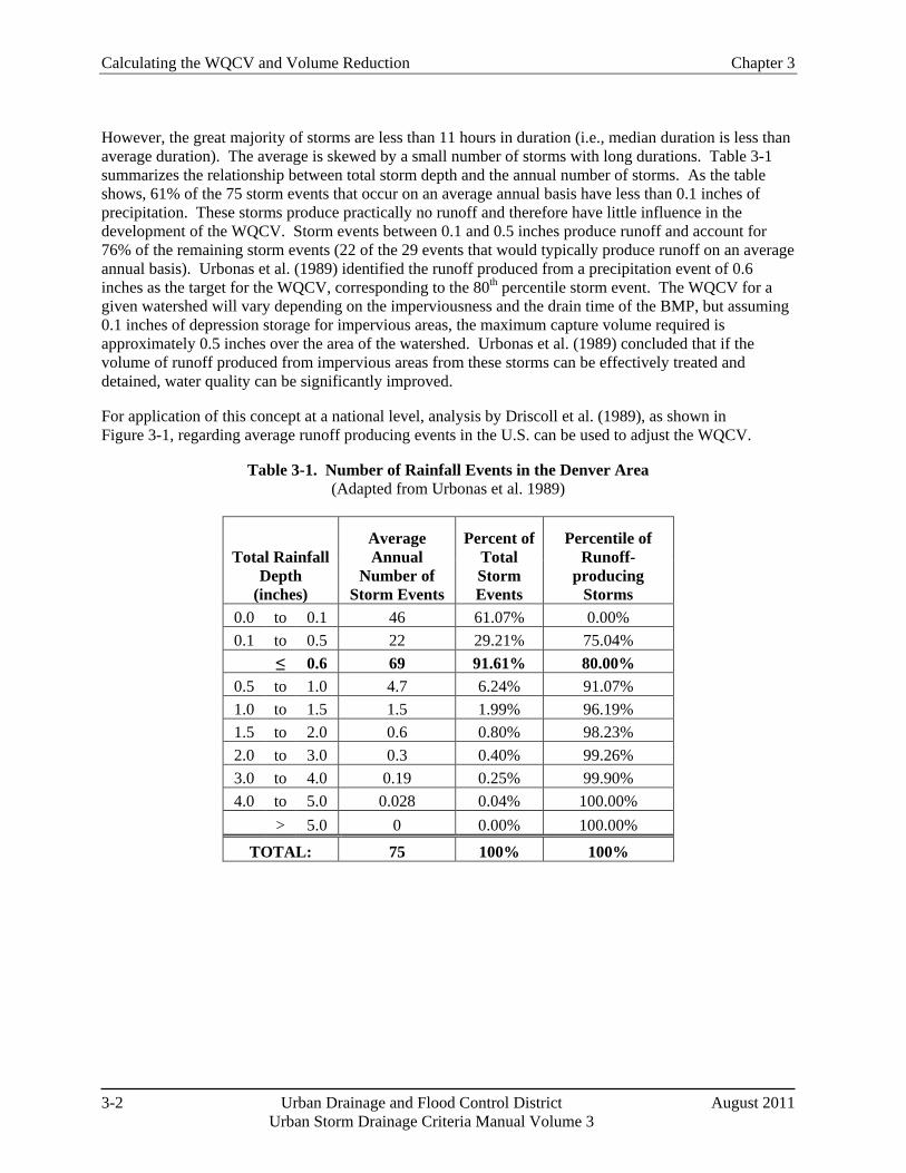
However, the great majority of storms are less than 11 hours in duration (i.e., median duration is less than average duration). The average is skewed by a small number of storms with long durations. Table 3-1 summarizes the relationship between total storm depth and the annual number of storms. As the table shows, 61% of the 75 storm events that occur on an average annual basis have less than 0.1 inches of precipitation. These storms produce practically no runoff and therefore have little influence in the development of the WQCV. Storm events between 0.1 and 0.5 inches produce runoff and account for 76% of the remaining storm events (22 of the 29 events that would typically produce runoff on an average annual basis). Urbonas et al. (1989) identified the runoff produced from a precipitation event of 0.6 inches as the target for the WQCV, corresponding to the 80th percentile storm event. The WQCV for a given watershed will vary depending on the imperviousness and the drain time of the BMP, but assuming 0.1 inches of depression storage for impervious areas, the maximum capture volume required is approximately 0.5 inches over the area of the watershed. Urbonas et al. (1989) concluded that if the volume of runoff produced from impervious areas from these storms can be effectively treated and detained, water quality can be significantly improved.
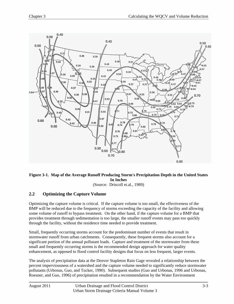
For application of this concept at a national level, analysis by Driscoll et al. (1989), as shown in Figure 3-1, regarding average runoff producing events in the U.S. can be used to adjust the WQCV.
Table 3-1. Number of Rainfall Events in the Denver Area (Adapted from Urbonas et al. 1989)
Total Rainfall Depth
(inches)
Average Annual
Number of Storm Events
Percent of Total Storm Events
Percentile of Runoff-
producing Storms
0.0 to 0.1 46 61.07% 0.00% 0.1 to 0.5 22 29.21% 75.04%
≤ 0.6 69 91.61% 80.00% 0.5 to 1.0 4.7 6.24% 91.07% 1.0 to 1.5 1.5 1.99% 96.19% 1.5 to 2.0 0.6 0.80% 98.23% 2.0 to 3.0 0.3 0.40% 99.26% 3.0 to 4.0 0.19 0.25% 99.90% 4.0 to 5.0 0.028 0.04% 100.00%
> 5.0 0 0.00% 100.00%
TOTAL: 75 100% 100%
Chapter 3 Calculating the WQCV and Volume Reduction
August 2011 Urban Drainage and Flood Control District 3-3 Urban Storm Drainage Criteria Manual Volume 3
Figure 3-1. Map of the Average Runoff Producing Storm's Precipitation Depth in the United States In Inches
(Source: Driscoll et.al., 1989)
2.2 Optimizing the Capture Volume
Optimizing the capture volume is critical. If the capture volume is too small, the effectiveness of the BMP will be reduced due to the frequency of storms exceeding the capacity of the facility and allowing some volume of runoff to bypass treatment. On the other hand, if the capture volume for a BMP that provides treatment through sedimentation is too large, the smaller runoff events may pass too quickly through the facility, without the residence time needed to provide treatment.
Small, frequently occurring storms account for the predominant number of events that result in stormwater runoff from urban catchments. Consequently, these frequent storms also account for a significant portion of the annual pollutant loads. Capture and treatment of the stormwater from these small and frequently occurring storms is the recommended design approach for water quality enhancement, as opposed to flood control facility designs that focus on less frequent, larger events.
The analysis of precipitation data at the Denver Stapleton Rain Gage revealed a relationship between the percent imperviousness of a watershed and the capture volume needed to significantly reduce stormwater pollutants (Urbonas, Guo, and Tucker, 1990). Subsequent studies (Guo and Urbonas, 1996 and Urbonas, Roesner, and Guo, 1996) of precipitation resulted in a recommendation by the Water Environment
Calculating the WQCV and Volume Reduction Chapter 3
3-4 Urban Drainage and Flood Control District August 2011 Urban Storm Drainage Criteria Manual Volume 3
Federation and American Society of Civil Engineers (1998) that stormwater quality treatment facilities (i.e., post-construction BMPs) be based on the capture and treatment of runoff from storms ranging in size from "mean" to "maximized1
2.3 Attenuation of the WQCV (BMP Drain Time)
" storms. The "mean" and "maximized" storm events represent the 70th and 90th percentile storms, respectively. As a result of these studies, water quality facilities for the Colorado Front Range are recommended to capture and treat the 80th percentile runoff event. Capturing and properly treating this volume should remove between 80 and 90% of the annual TSS load, while doubling the capture volume was estimated to increase the removal rate by only 1 to 2%.
The WQCV must be released over an extended period to provide effective pollutant removal for post-construction BMPs that use sedimentation (i.e., extended detention basin, retention ponds and constructed wetland ponds). A field study of basins with extended detention in the Washington, D.C. area identified an average drain time of 24 hours to be effective for extended detention basins. This generally equates to a 40-hour drain time for the brim-full basin. Retention ponds and constructed wetland basins have reduced drain times (12 hours and 24 hours, respectively) because the hydraulic residence time of the effluent is essentially increased due to the mixing of the inflow with the permanent pool.
When pollutant removal is achieved primarily through filtration such as in a sand filter or rain garden BMP, an extended drain time is still recommended to promote stability of downstream drainageways, but it can be reduced because it is not needed for effective pollutant removal. In addition to counteracting hydromodification, attenuation in filtering BMPs can also improve pollutant removal by increasing contact time, which can aid adsorption/absorption processes depending on the media. The minimum recommended drain time for a post-construction BMP is 12 hours; however, this minimum value should only be used for BMPs that do not rely fully or partially on sedimentation for pollutant removal.
2.4 Excess Urban Runoff Volume (EURV) and Full Spectrum Detention
The EURV represents the difference between the developed and pre-developed runoff volume for the range of storms that produce runoff from pervious land surfaces (generally greater than the 2-year event). The EURV is relatively constant for a given imperviousness over a wide range of storm events. This is a companion concept to the WQCV. The EURV is a greater volume than the WQCV and is detained over a longer time. It typically allows for the recommended drain time of the WQCV and is used to better replicate peak discharge in receiving waters for runoff events exceeding the WQCV. The EURV is associated with Full Spectrum Detention, a simplified sizing method for both water quality and flood control detention. Designing a detention basin to capture the EURV and release it slowly (at a rate similar to WQCV release) results in storms smaller than the 2-year event being reduced to flow rates much less than the threshold value for erosion in most drainageways. In addition, by incorporating an outlet structure designed per the criteria in this manual including an orifice or weir that limits 100-year runoff to the allowable release rate, the storms greater than the 2-year event will be reduced to discharge rates and hydrograph shapes that approximate pre-developed conditions. This reduces the likelihood that runoff hydrographs from multiple basins will combine to produce greater discharges than pre-developed conditions.
For additional information on the EURV and Full Spectrum Detention, including calculation procedures, please refer to the Storage chapter of Volume 2. 1 The term "maximized storm" refers to the optimization of the storage volume of a BMP. The WQCV for the "maximized" storm represents the point of diminishing returns in terms of the number of storm events and volume of runoff fully treated versus the storage volume provided.
Chapter 3 Calculating the WQCV and Volume Reduction
August 2011 Urban Drainage and Flood Control District 3-5 Urban Storm Drainage Criteria Manual Volume 3
3.0 Calculation of the WQCV The first step in estimating the magnitude of runoff from a site is to estimate the site's total imperviousness. The total imperviousness of a site is the weighted average of individual areas of like imperviousness. For instance, according to Table RO-3 in the Runoff chapter of Volume 1 of this manual, paved streets (and parking lots) have an imperviousness of 100%; drives, walks and roofs have an imperviousness of 90%; and lawn areas have an imperviousness of 0%. The total imperviousness of a site can be determined taking an area-weighted average of all of the impervious and pervious areas. When measures are implemented minimize directly connected impervious area (MDCIA), the imperviousness used to calculate the WQCV is the "effective imperviousness." Sections 4 and 5 of this chapter provide guidance and examples for calculating effective imperviousness and adjusting the WQCV to reflect decreases in effective imperviousness.
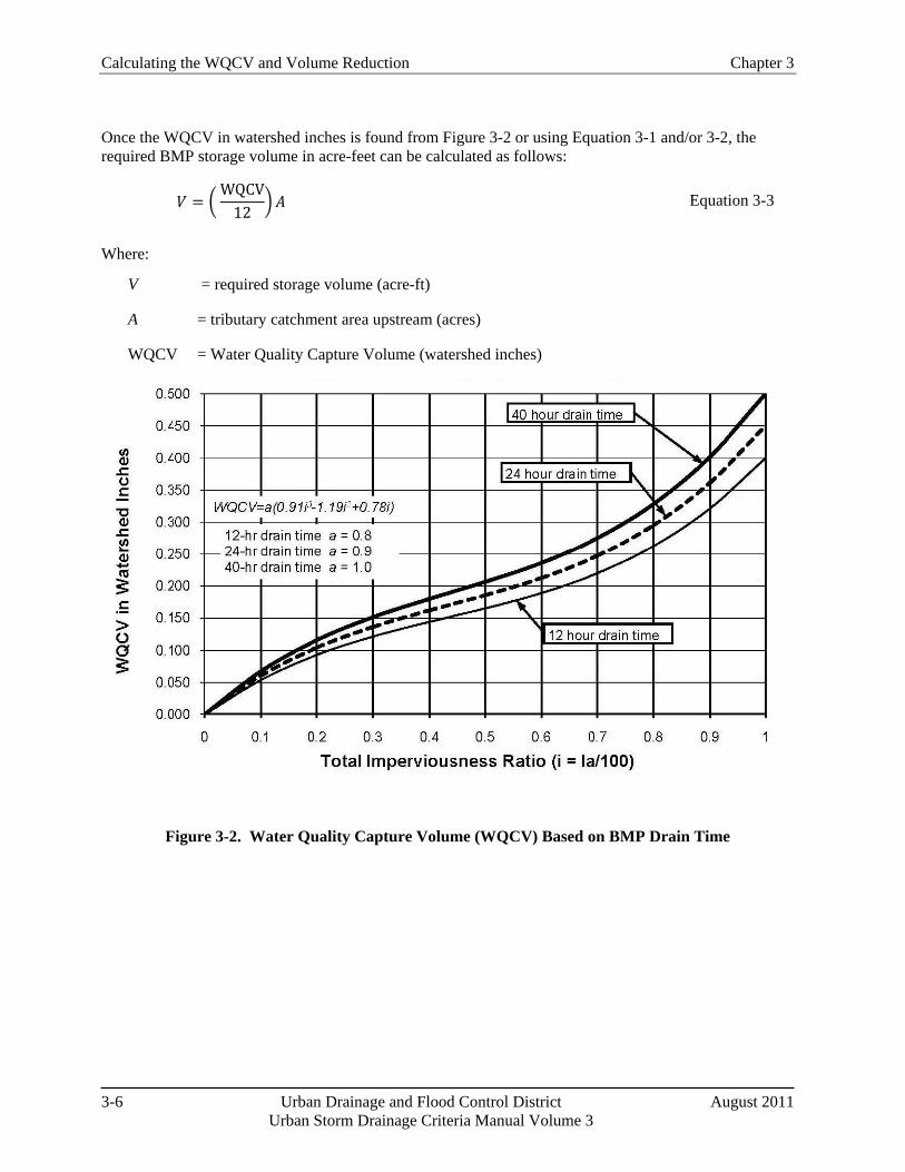
The WQCV is calculated as a function of imperviousness and BMP drain time using Equation 3-1, and as shown in Figure 3-2:
WQCV = 𝑎(0.91𝐼3 − 1.19𝐼2 + 0.78𝐼) Equation 3-1
Where:
WQCV = Water Quality Capture Volume (watershed inches)
a = Coefficient corresponding to WQCV drain time (Table 3-2)
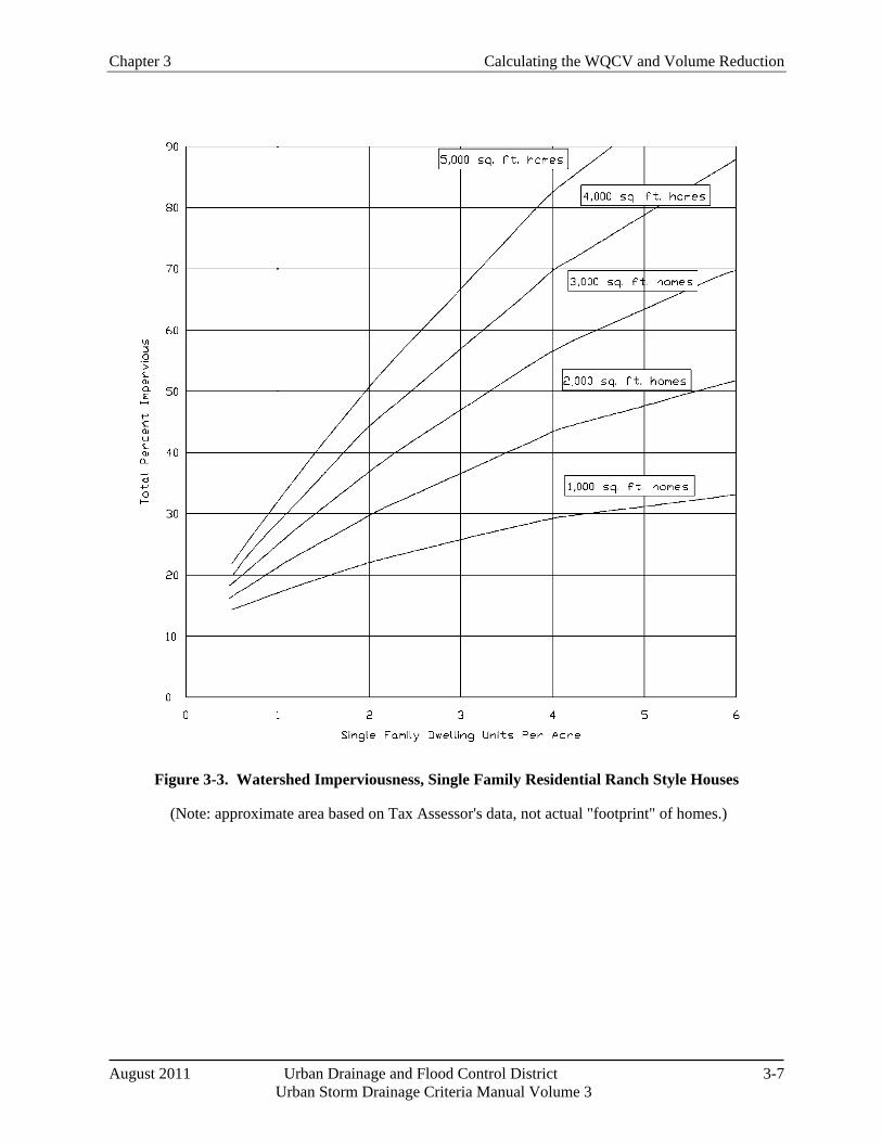
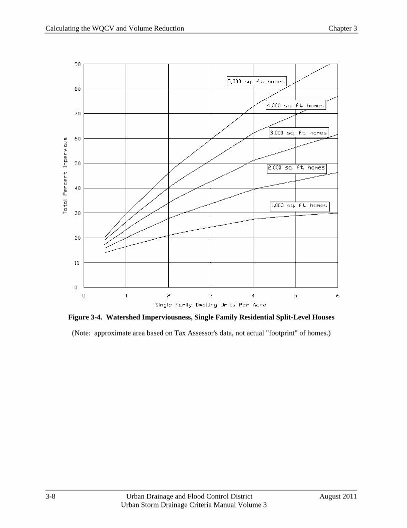
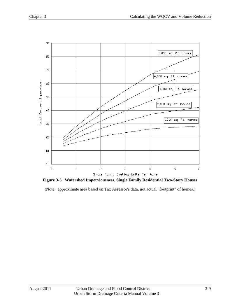
I = Imperviousness (%/100) (see Figures 3-3 through 3-5 [single family land use] and /or the Runoff chapter of Volume 1[other typical land uses])
Table 3-2. Drain Time Coefficients for WQCV Calculations
Drain Time (hrs) Coefficient, a 12 hours 0.8 24 hours 0.9 40 hours 1.0
Figure 3-2, which illustrates the relationship between imperviousness and WQCV for various drain times, is appropriate for use in Colorado's high plains near the foothills. For other portions of Colorado or United States, the WQCV obtained from this figure can be adjusted using the following relationships:
WQCVother = 𝑑6 �WQCV0.43
� Equation 3-2
Where:
WQCV = WQCV calculated using Equation 3-1 or Figure 3-2 (watershed inches)
WQCVother = WQCV outside of Denver region (watershed inches)
d6 = depth of average runoff producing storm from Figure 3-1 (watershed inches)
Calculating the WQCV and Volume Reduction Chapter 3
3-6 Urban Drainage and Flood Control District August 2011 Urban Storm Drainage Criteria Manual Volume 3
Once the WQCV in watershed inches is found from Figure 3-2 or using Equation 3-1 and/or 3-2, the required BMP storage volume in acre-feet can be calculated as follows:
𝑉 = � WQCV
12�𝐴 Equation 3-3
Where:
V = required storage volume (acre-ft)
A = tributary catchment area upstream (acres)
WQCV = Water Quality Capture Volume (watershed inches)
Figure 3-2. Water Quality Capture Volume (WQCV) Based on BMP Drain Time
Chapter 3 Calculating the WQCV and Volume Reduction
August 2011 Urban Drainage and Flood Control District 3-7 Urban Storm Drainage Criteria Manual Volume 3
Figure 3-3. Watershed Imperviousness, Single Family Residential Ranch Style Houses
(Note: approximate area based on Tax Assessor's data, not actual "footprint" of homes.)
Calculating the WQCV and Volume Reduction Chapter 3
3-8 Urban Drainage and Flood Control District August 2011 Urban Storm Drainage Criteria Manual Volume 3
Figure 3-4. Watershed Imperviousness, Single Family Residential Split-Level Houses
(Note: approximate area based on Tax Assessor's data, not actual "footprint" of homes.)
Chapter 3 Calculating the WQCV and Volume Reduction
August 2011 Urban Drainage and Flood Control District 3-9 Urban Storm Drainage Criteria Manual Volume 3
Figure 3-5. Watershed Imperviousness, Single Family Residential Two-Story Houses
(Note: approximate area based on Tax Assessor's data, not actual "footprint" of homes.)
Calculating the WQCV and Volume Reduction Chapter 3
3-10 Urban Drainage and Flood Control District August 2011 Urban Storm Drainage Criteria Manual Volume 3
Defining Effective Imperviousness
The concepts discussed in this section are dependent on the concept of effective imperviousness. This term refers to impervious areas that contribute surface runoff to the drainage system. For the purposes of this manual, effective imperviousness includes directly connected impervious area and portions of the unconnected impervious area that also contribute to runoff from a site. For small, frequently occurring events, the effective imperviousness may be equivalent to directly connected impervious area since runoff from unconnected impervious areas may infiltrate into receiving pervious areas; however, for larger events, the effective imperviousness is increased to account for runoff from unconnected impervious areas that exceeds the infiltration capacity of the receiving pervious area. This means that the calculation of effective imperviousness is associated with a specific return period.
Note: Users should be aware that some national engineering literature defines effective impervious more narrowly to include only directly connected impervious area.
4.0 Quantifying Volume Reduction Volume reduction is an important part of the Four Step Process and is fundamental to effective stormwater management. Quantifying volume reduction associated with MDCIA, LID practices and other BMPs is important for watershed-level master planning and also for conceptual and final site design. It also allows the engineer to evaluate and compare the benefits of various volume reduction practices. This section describes the conceptual model for evaluating volume reduction and provides tools for quantifying volume reduction using three different approaches, depending on the size of the watershed, complexity of the design, and experience level of the user. In this section volume reduction is evaluated at the watershed level using CUHP and on the site level using SWMM or design curves and spreadsheets developed from SWMM analysis.
4.1 Conceptual Model for Volume Reduction BMPs—Cascading Planes
The hydrologic response of a watershed during a storm event is characterized by factors including shape, slope, area, imperviousness (connected and disconnected) and other factors (Guo 2006). As previously discussed, total imperviousness of a watershed can be determined by delineating roofs, drives, walks and other impervious areas within a watershed and dividing the sum of these impervious areas by the total watershed area. In the past, total imperviousness was often used for calculation of peak flow rates for design events and storage requirements for water quality and flood control purposes. This is a reasonable approach when much of the impervious area in a watershed is directly connected to the drainage system; however, when the unconnected impervious area in a catchment is significant, using total imperviousness will result in over-calculation of peak flow rates and storage requirements.
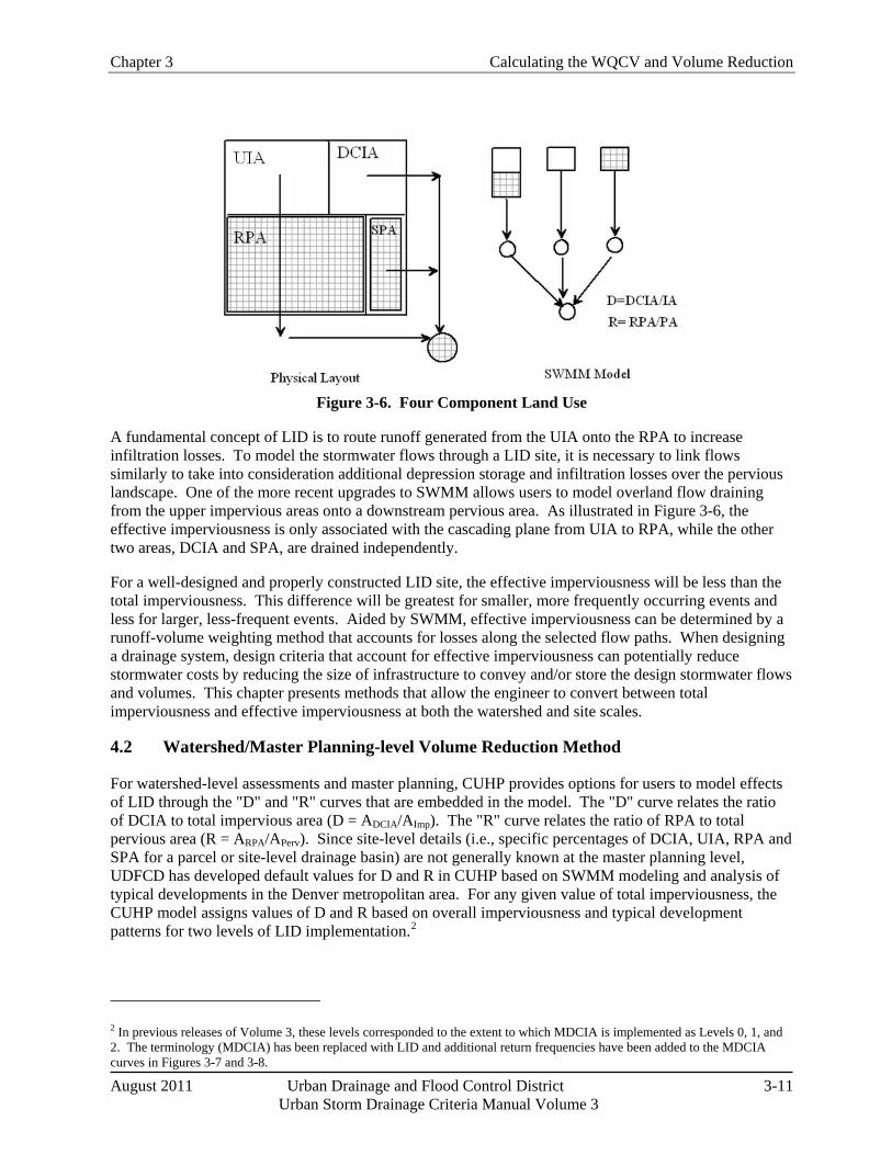
To evaluate the effects of MDCIA and other LID practices, UDFCD has performed modeling using SWMM to develop tools for planners and designers, both at the watershed/master planning level where site-specific details have not been well defined, and at the site level, where plans are at more advanced stages. Unlike many conventional stormwater models, SWMM allows for a relatively complex evaluation of flow paths through the on-site stormwater BMP layout. Conceptually, an urban watershed can be divided into four land use areas that drain to the common outfall point as shown in Figure 3-6, including:
Directly Connected Impervious Area (DCIA)
Unconnected Impervious Area (UIA)
Receiving Pervious Area (RPA)
Separate Pervious Area (SPA)
Chapter 3 Calculating the WQCV and Volume Reduction
August 2011 Urban Drainage and Flood Control District 3-11 Urban Storm Drainage Criteria Manual Volume 3
Figure 3-6. Four Component Land Use
A fundamental concept of LID is to route runoff generated from the UIA onto the RPA to increase infiltration losses. To model the stormwater flows through a LID site, it is necessary to link flows similarly to take into consideration additional depression storage and infiltration losses over the pervious landscape. One of the more recent upgrades to SWMM allows users to model overland flow draining from the upper impervious areas onto a downstream pervious area. As illustrated in Figure 3-6, the effective imperviousness is only associated with the cascading plane from UIA to RPA, while the other two areas, DCIA and SPA, are drained independently.
For a well-designed and properly constructed LID site, the effective imperviousness will be less than the total imperviousness. This difference will be greatest for smaller, more frequently occurring events and less for larger, less-frequent events. Aided by SWMM, effective imperviousness can be determined by a runoff-volume weighting method that accounts for losses along the selected flow paths. When designing a drainage system, design criteria that account for effective imperviousness can potentially reduce stormwater costs by reducing the size of infrastructure to convey and/or store the design stormwater flows and volumes. This chapter presents methods that allow the engineer to convert between total imperviousness and effective imperviousness at both the watershed and site scales.
4.2 Watershed/Master Planning-level Volume Reduction Method
For watershed-level assessments and master planning, CUHP provides options for users to model effects of LID through the "D" and "R" curves that are embedded in the model. The "D" curve relates the ratio of DCIA to total impervious area (D = ADCIA/AImp). The "R" curve relates the ratio of RPA to total pervious area (R = ARPA/APerv). Since site-level details (i.e., specific percentages of DCIA, UIA, RPA and SPA for a parcel or site-level drainage basin) are not generally known at the master planning level, UDFCD has developed default values for D and R in CUHP based on SWMM modeling and analysis of typical developments in the Denver metropolitan area. For any given value of total imperviousness, the CUHP model assigns values of D and R based on overall imperviousness and typical development patterns for two levels of LID implementation.2
2 In previous releases of Volume 3, these levels corresponded to the extent to which MDCIA is implemented as Levels 0, 1, and 2. The terminology (MDCIA) has been replaced with LID and additional return frequencies have been added to the MDCIA curves in Figures 3-7 and 3-8.
Calculating the WQCV and Volume Reduction Chapter 3
3-12 Urban Drainage and Flood Control District August 2011 Urban Storm Drainage Criteria Manual Volume 3
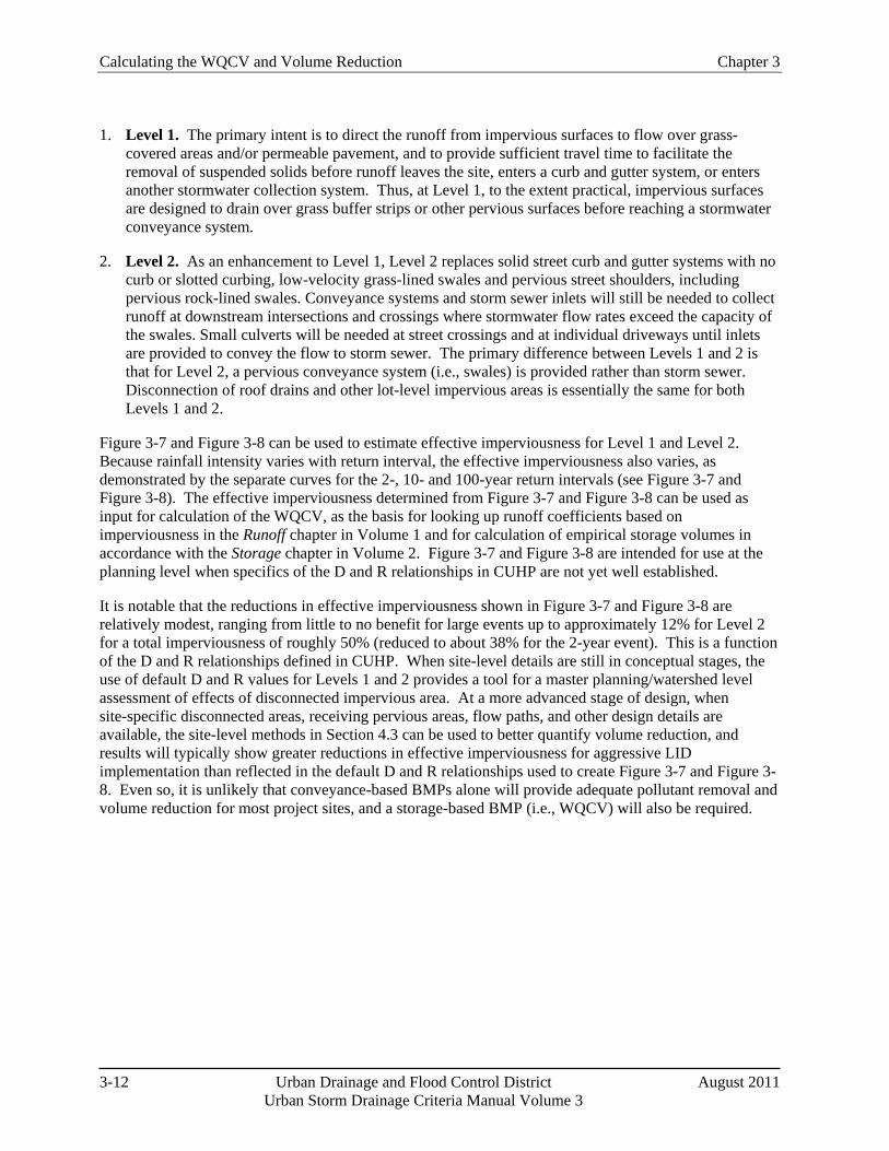
1. Level 1. The primary intent is to direct the runoff from impervious surfaces to flow over grass-covered areas and/or permeable pavement, and to provide sufficient travel time to facilitate the removal of suspended solids before runoff leaves the site, enters a curb and gutter system, or enters another stormwater collection system. Thus, at Level 1, to the extent practical, impervious surfaces are designed to drain over grass buffer strips or other pervious surfaces before reaching a stormwater conveyance system.
2. Level 2. As an enhancement to Level 1, Level 2 replaces solid street curb and gutter systems with no curb or slotted curbing, low-velocity grass-lined swales and pervious street shoulders, including pervious rock-lined swales. Conveyance systems and storm sewer inlets will still be needed to collect runoff at downstream intersections and crossings where stormwater flow rates exceed the capacity of the swales. Small culverts will be needed at street crossings and at individual driveways until inlets are provided to convey the flow to storm sewer. The primary difference between Levels 1 and 2 is that for Level 2, a pervious conveyance system (i.e., swales) is provided rather than storm sewer. Disconnection of roof drains and other lot-level impervious areas is essentially the same for both Levels 1 and 2.
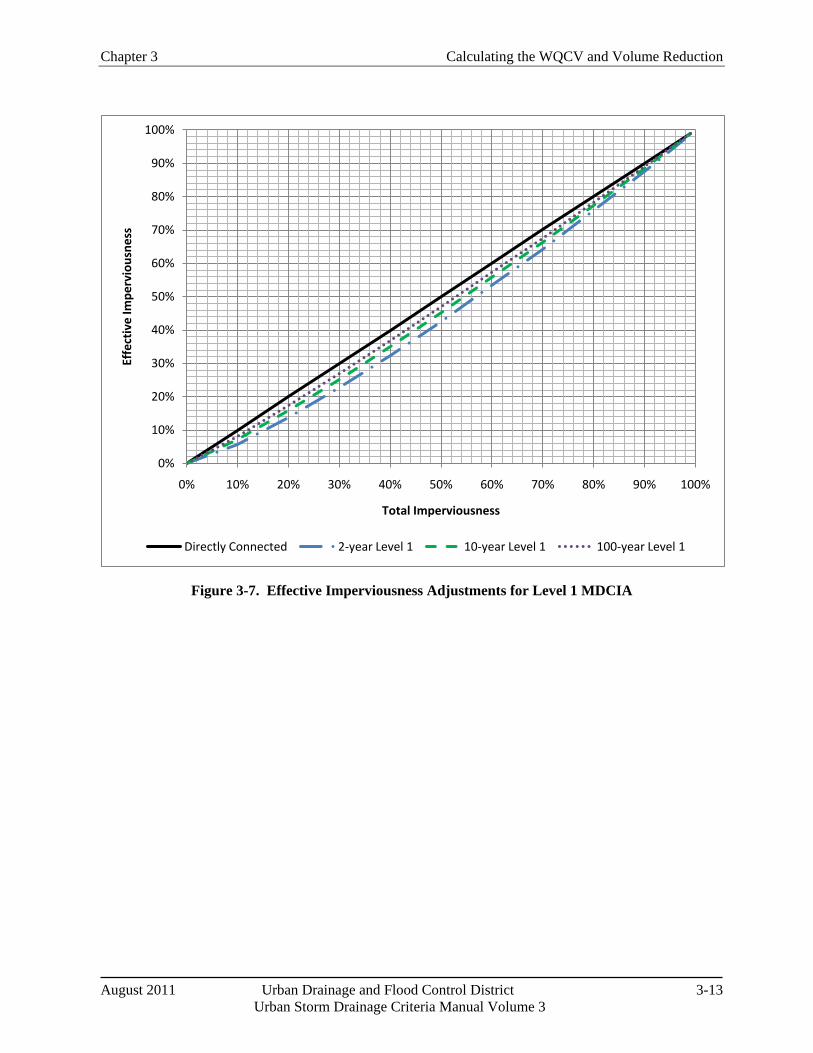
Figure 3-7 and Figure 3-8 can be used to estimate effective imperviousness for Level 1 and Level 2. Because rainfall intensity varies with return interval, the effective imperviousness also varies, as demonstrated by the separate curves for the 2-, 10- and 100-year return intervals (see Figure 3-7 and Figure 3-8). The effective imperviousness determined from Figure 3-7 and Figure 3-8 can be used as input for calculation of the WQCV, as the basis for looking up runoff coefficients based on imperviousness in the Runoff chapter in Volume 1 and for calculation of empirical storage volumes in accordance with the Storage chapter in Volume 2. Figure 3-7 and Figure 3-8 are intended for use at the planning level when specifics of the D and R relationships in CUHP are not yet well established.
It is notable that the reductions in effective imperviousness shown in Figure 3-7 and Figure 3-8 are relatively modest, ranging from little to no benefit for large events up to approximately 12% for Level 2 for a total imperviousness of roughly 50% (reduced to about 38% for the 2-year event). This is a function of the D and R relationships defined in CUHP. When site-level details are still in conceptual stages, the use of default D and R values for Levels 1 and 2 provides a tool for a master planning/watershed level assessment of effects of disconnected impervious area. At a more advanced stage of design, when site-specific disconnected areas, receiving pervious areas, flow paths, and other design details are available, the site-level methods in Section 4.3 can be used to better quantify volume reduction, and results will typically show greater reductions in effective imperviousness for aggressive LID implementation than reflected in the default D and R relationships used to create Figure 3-7 and Figure 3-8. Even so, it is unlikely that conveyance-based BMPs alone will provide adequate pollutant removal and volume reduction for most project sites, and a storage-based BMP (i.e., WQCV) will also be required.
Chapter 3 Calculating the WQCV and Volume Reduction
August 2011 Urban Drainage and Flood Control District 3-13 Urban Storm Drainage Criteria Manual Volume 3
Figure 3-7. Effective Imperviousness Adjustments for Level 1 MDCIA
0%
10%
20%
30%
40%
50%
60%
70%
80%
90%
100%
0% 10% 20% 30% 40% 50% 60% 70% 80% 90% 100%
Effe
ctiv
e Im
perv
ious
ness
Total Imperviousness
Directly Connected 2-year Level 1 10-year Level 1 100-year Level 1
Calculating the WQCV and Volume Reduction Chapter 3
3-14 Urban Drainage and Flood Control District August 2011 Urban Storm Drainage Criteria Manual Volume 3
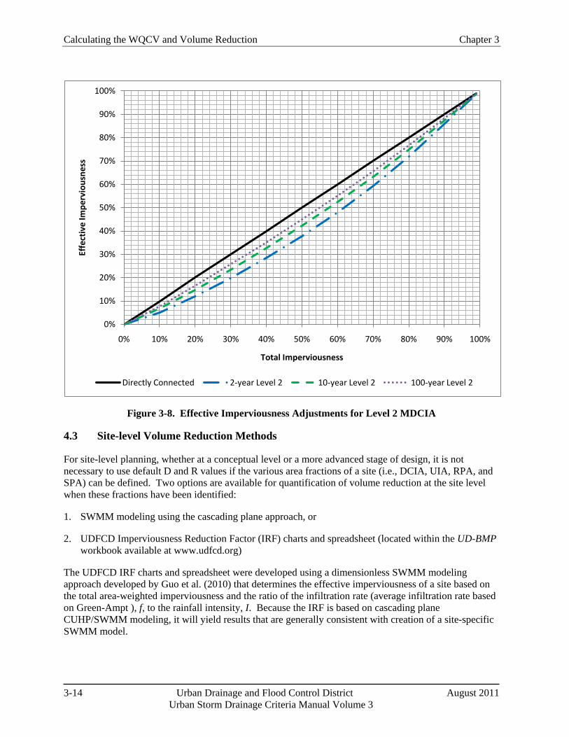
Figure 3-8. Effective Imperviousness Adjustments for Level 2 MDCIA
4.3 Site-level Volume Reduction Methods
For site-level planning, whether at a conceptual level or a more advanced stage of design, it is not necessary to use default D and R values if the various area fractions of a site (i.e., DCIA, UIA, RPA, and SPA) can be defined. Two options are available for quantification of volume reduction at the site level when these fractions have been identified:
1. SWMM modeling using the cascading plane approach, or
2. UDFCD Imperviousness Reduction Factor (IRF) charts and spreadsheet (located within the UD-BMP workbook available at www.udfcd.org)
The UDFCD IRF charts and spreadsheet were developed using a dimensionless SWMM modeling approach developed by Guo et al. (2010) that determines the effective imperviousness of a site based on the total area-weighted imperviousness and the ratio of the infiltration rate (average infiltration rate based on Green-Ampt ), f, to the rainfall intensity, I. Because the IRF is based on cascading plane CUHP/SWMM modeling, it will yield results that are generally consistent with creation of a site-specific SWMM model.
0%
10%
20%
30%
40%
50%
60%
70%
80%
90%
100%
0% 10% 20% 30% 40% 50% 60% 70% 80% 90% 100%
Effe
ctiv
e Im
perv
ious
ness
Total Imperviousness
Directly Connected 2-year Level 2 10-year Level 2 100-year Level 2
Chapter 3 Calculating the WQCV and Volume Reduction
August 2011 Urban Drainage and Flood Control District 3-15 Urban Storm Drainage Criteria Manual Volume 3
To apply either of the above methods, a project site must first be divided into sub-watersheds based on topography and drainage patterns. For each sub-watershed, the areas of DCIA, UIA, RPA and SPA should be calculated. Sub-watersheds (and associated BMPs) will fall into one of two categories based on the types of BMPs used:
1. Conveyance-based: Conveyance-based BMPs include grass swales, vegetated buffers, and disconnection of roof drains and other impervious areas to drain to pervious areas (UDFCD 1999a). Conveyance based BMPs may have some incidental, short-term storage in the form of channel storage or shallow ponding but do not provide the WQCV, EURV or flood-control detention volume.
2. Storage-based: Storage-based BMPs include rain gardens, permeable pavement systems as detailed in this manual, extended detention basins and other BMPs in this manual that provide the WQCV, EURV or flood control detention volume.
4.3.1 SWMM Modeling Using Cascading Planes
Because of complexities of modeling LID and other BMPs using SWMM, the cascading planes alternative for site-level volume reduction analysis is recommended only for experienced users. Guidance for conveyance- and storage-based modeling includes these steps:
1. Each sub-watershed should be conceptualized as shown in Figure 3-6. Two approaches can be used in SWMM to achieve this:
Create two SWMM sub-catchments for each sub-watershed, one with UIA 100% routed to RPA and the other with DCIA and SPA independently routed to the outlet, or
Use a single SWMM sub-catchment to represent the sub-watershed and use the SWMM internal routing option to differentiate between DCIA and UIA. This option should only be used when a large portion of the pervious area on a site is RPA and there is very little SPA since the internal routing does not have the ability to differentiate between SPA and RPA (i.e., the UIA is routed to the entire pervious area, potentially overestimating infiltration losses).
2. Once the subwatershed is set up to represent UIA, DCIA, RPA and SPA in SWMM, the rainfall distribution should be directly input to SWMM. As an alternative, SWMM can be used only for routing with rainfall-runoff handled in CUHP using sub-watershed specific D and R values to define fractions of pervious and impervious areas.
3. Parameters for infiltration, depression storage and other input parameters should be selected in accordance with the guidance in the Runoff chapter of Volume 1.
4. For storage-based BMPs, there are two options for representing the WQCV:
The pervious area depression storage value for the RPA can be increased to represent the WQCV. This approach is generally applicable to storage-based BMPs that promote infiltration such as rain gardens, permeable pavement systems with storage or sand filters. This adjustment should not be used when a storage-based BMP has a well-defined outlet and a stage-storage-discharge relationship that can be entered into SWMM.
Calculating the WQCV and Volume Reduction Chapter 3
3-16 Urban Drainage and Flood Control District August 2011 Urban Storm Drainage Criteria Manual Volume 3
The WQCV can be modeled as a storage unit with an outlet in SWMM. This option is preferred for storage-based BMPs with well defined stage-storage-discharge relationships such as extended detention basins.
These guidelines are applicable for EPA SWMM Version 5.0.018 and earlier versions going back to EPA SWMM 5.0. EPA is currently developing a version of EPA SWMM with enhanced LID modeling capabilities; however, this version had not been fully vetted at the time this manual was released.
4.3.2 IRF Charts and Spreadsheet
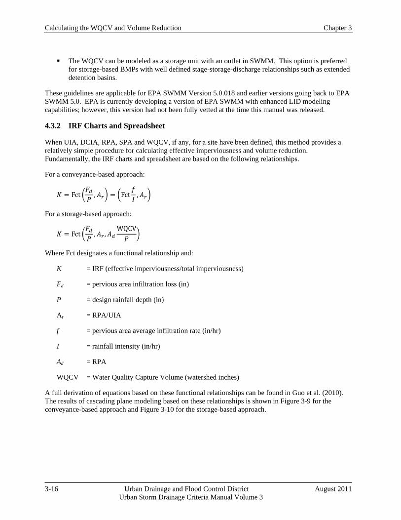
When UIA, DCIA, RPA, SPA and WQCV, if any, for a site have been defined, this method provides a relatively simple procedure for calculating effective imperviousness and volume reduction. Fundamentally, the IRF charts and spreadsheet are based on the following relationships.
For a conveyance-based approach:
𝐾 = Fct ��𝐹𝑑𝑃� ,𝐴𝑟� = ��Fct
𝑓𝐼� ,𝐴𝑟�
For a storage-based approach:
𝐾 = Fct ��𝐹𝑑𝑃� ,𝐴𝑟 ,𝐴𝑑
WQCV𝑃
�
Where Fct designates a functional relationship and:
K = IRF (effective imperviousness/total imperviousness)
Fd = pervious area infiltration loss (in)
P = design rainfall depth (in)
Ar = RPA/UIA
f = pervious area average infiltration rate (in/hr)
I = rainfall intensity (in/hr)
Ad = RPA
WQCV = Water Quality Capture Volume (watershed inches)
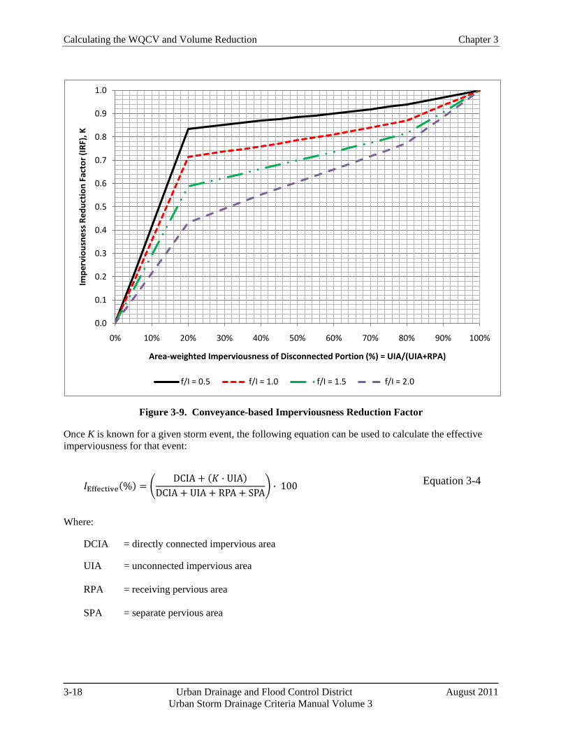
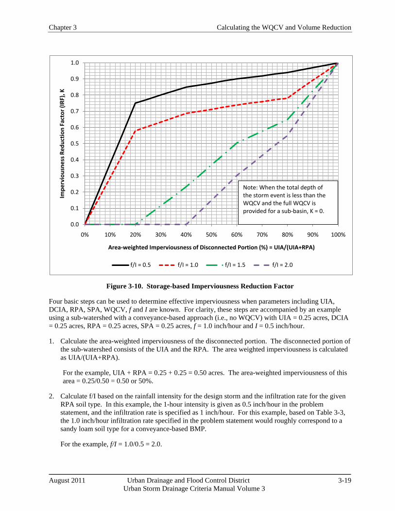
A full derivation of equations based on these functional relationships can be found in Guo et al. (2010). The results of cascading plane modeling based on these relationships is shown in Figure 3-9 for the conveyance-based approach and Figure 3-10 for the storage-based approach.
Chapter 3 Calculating the WQCV and Volume Reduction
August 2011 Urban Drainage and Flood Control District 3-17 Urban Storm Drainage Criteria Manual Volume 3
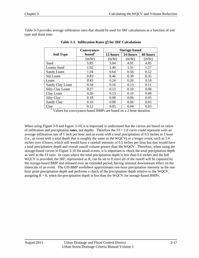
Table 3-3 provides average infiltration rates that should be used for IRF calculations as a function of soil type and drain time.
Table 3-3. Infiltration Rates (f) for IRF Calculations
Soil Type Conveyance-
based1 Storage-based
12-hours 24-hours 40-hours (in/hr) (in/hr) (in/hr) (in/hr)
Sand 5.85 5.04 4.91 4.85 Loamy Sand 1.92 1.40 1.31 1.27 Sandy Loam 1.04 0.64 0.56 0.52 Silt Loam 0.83 0.46 0.39 0.35 Loam 0.43 0.24 0.20 0.18 Sandy Clay Loam 0.34 0.16 0.13 0.11 Silty Clay Loam 0.27 0.13 0.10 0.08 Clay Loam 0.26 0.13 0.10 0.08 Silty Clay 0.18 0.08 0.06 0.05 Sandy Clay 0.16 0.08 0.06 0.05 Clay 0.12 0.05 0.04 0.03
1 Values for conveyance-based BMPs are based on a 2-hour duration.
When using Figure 3-9 and Figure 3-10, it is important to understand that the curves are based on ratios of infiltration and precipitation rates, not depths. Therefore the f/I = 2.0 curve could represent soils an average infiltration rate of 1 inch per hour and an event with a total precipitation of 0.5 inches in 1 hour (i.e., an event with a total depth that is roughly the same as the WQCV) or a longer event, such as 2.0 inches over 4 hours, which still would have a rainfall intensity of 0.5 inches per hour but that would have a total precipitation depth and overall runoff volume greater than the WQCV. Therefore, when using the storage-based curves in Figure 3-10 for small events, it is important to check the total precipitation depth as well as the f/I ratio. In cases where the total precipitation depth is less than 0.6 inches and the full WQCV is provided, the IRF, represented as K, can be set to 0 since all of the runoff will be captured by the storage-based BMP and released over an extended period, having minimal downstream effect on the timescale of an event. The UD-BMP worksheet approximates one-hour precipitation intensity as the one hour point precipitation depth and performs a check of the precipitation depth relative to the WQCV, assigning K = 0, when the precipitation depth is less than the WQCV for storage-based BMPs.
Calculating the WQCV and Volume Reduction Chapter 3
3-18 Urban Drainage and Flood Control District August 2011 Urban Storm Drainage Criteria Manual Volume 3
Figure 3-9. Conveyance-based Imperviousness Reduction Factor
Once K is known for a given storm event, the following equation can be used to calculate the effective imperviousness for that event:
𝐼Effective(%) = �DCIA + (𝐾 ∙ UIA)
DCIA + UIA + RPA + SPA� ∙ 100 Equation 3-4
Where:
DCIA = directly connected impervious area
UIA = unconnected impervious area RPA = receiving pervious area SPA = separate pervious area
0.0
0.1
0.2
0.3
0.4
0.5
0.6
0.7
0.8
0.9
1.0
0% 10% 20% 30% 40% 50% 60% 70% 80% 90% 100%
Impe
rvio
usne
ss R
educ
tion
Fac
tor (
IRF)
, K
Area-weighted Imperviousness of Disconnected Portion (%) = UIA/(UIA+RPA)
f/I = 0.5 f/I = 1.0 f/I = 1.5 f/I = 2.0
Chapter 3 Calculating the WQCV and Volume Reduction
August 2011 Urban Drainage and Flood Control District 3-19 Urban Storm Drainage Criteria Manual Volume 3
Figure 3-10. Storage-based Imperviousness Reduction Factor
Four basic steps can be used to determine effective imperviousness when parameters including UIA, DCIA, RPA, SPA, WQCV, f and I are known. For clarity, these steps are accompanied by an example using a sub-watershed with a conveyance-based approach (i.e., no WQCV) with UIA = 0.25 acres, DCIA = 0.25 acres, RPA = 0.25 acres, SPA = 0.25 acres, f = 1.0 inch/hour and I = 0.5 inch/hour.
1. Calculate the area-weighted imperviousness of the disconnected portion. The disconnected portion of the sub-watershed consists of the UIA and the RPA. The area weighted imperviousness is calculated as UIA/(UIA+RPA).
For the example, UIA + RPA = 0.25 + 0.25 = 0.50 acres. The area-weighted imperviousness of this area = 0.25/0.50 = 0.50 or 50%.
2. Calculate f/I based on the rainfall intensity for the design storm and the infiltration rate for the given RPA soil type. In this example, the 1-hour intensity is given as 0.5 inch/hour in the problem statement, and the infiltration rate is specified as 1 inch/hour. For this example, based on Table 3-3, the 1.0 inch/hour infiltration rate specified in the problem statement would roughly correspond to a sandy loam soil type for a conveyance-based BMP.
For the example, f/I = 1.0/0.5 = 2.0.
0.0
0.1
0.2
0.3
0.4
0.5
0.6
0.7
0.8
0.9
1.0
0% 10% 20% 30% 40% 50% 60% 70% 80% 90% 100%
Impe
rvio
usne
ss R
educ
tion
Fac
tor (
IRF)
, K
Area-weighted Imperviousness of Disconnected Portion (%) = UIA/(UIA+RPA)
f/I = 0.5 f/I = 1.0 f/I = 1.5 f/I = 2.0
Note: When the total depth of the storm event is less than the WQCV and the full WQCV is provided for a sub-basin, K = 0.
Calculating the WQCV and Volume Reduction Chapter 3
3-20 Urban Drainage and Flood Control District August 2011 Urban Storm Drainage Criteria Manual Volume 3
For simplicity, the 1-hour rainfall intensity can be approximated as the 1-hour point precipitation depth for a given frequency. The 1-hour point precipitation values can be determined from Rainfall Depth-Duration-Frequency figures in the Rainfall chapter of Volume 1.
3. Using the appropriate figure (Figure 3-9 for the conveyance-based approach or Figure 3-10 for the storage-based approach), determine the Imperviousness Reduction Factor, K, corresponding to where the appropriate f/I line would be intersected by the x-axis value for area-weighted imperviousness. Note: Figure 3-10 for the storage-based approach should only be used if the full WQCV is provided for the sub-watershed. If quantification of volume reduction benefits of only a fraction of the WQCV (one-half for example) is required, Figure 3-10 is not applicable and SWMM modeling will be required.
For the example, the K value corresponding to f/I = 2.0 and an area-weighted imperviousness of 50% using the conveyance-based chart, Figure 3-9, is 0.60. It is very important to note that this K value applies only to the disconnected portion of the sub-watershed (i.e., UIA + RPA).
4. Calculate the effective imperviousness of the sub-watershed. This calculation must factor in both connected and disconnected portions of the site:
𝐼Effective(%) = �DCIA + (𝐾 ∙ UIA)
DCIA + UIA + RPA + SPA� ∙ 100
For the example, with DCIA = UIA = RPA = SPA = 0.25 acres and K = 0.60:
𝐼Effectiv𝑒(%) = �0.25 + (0.60 ∙ 0.25)
0.25 + 0.25 + 0.25 + 0.25� ∙ 100 = 40%
This can be compared to the total area-weighted imperviousness for the sub-watershed = (DCIA + UIA)/ (DCIA + UIA + RPA + SPA) × 100% = 50%.
To calculate volume reduction benefits associated with conveyance- or storage-based approaches, the effective imperviousness values determined according to this procedure (or using the spreadsheet tool UD-BMP) can be used in WQCV calculations and detention storage equations, such as the empirical storage equations in the Storage chapter of Volume 1. The WQCV and detention volume requirements calculated using the effective imperviousness can be compared with the same calculations using total sub-watershed imperviousness to determine potential volume reductions.
Section 5.2 provides an example of the storage-based approach to complement the conveyance-based example above, as well as guidance for using the spreadsheet tool.
4.4 Other Types of Credits for Volume Reduction BMPs/LID
In addition to facility sizing reduction credits following the quantitative procedures in Section 4.3, communities can also consider other incentives to encourage volume reduction practices. Such incentives will depend on the policies and objectives of local governments. Representative examples that could be considered include:
Stormwater utility fee credits.
Lower stormwater system development fees when certain minimum criteria are met.
Chapter 3 Calculating the WQCV and Volume Reduction
August 2011 Urban Drainage and Flood Control District 3-21 Urban Storm Drainage Criteria Manual Volume 3
Density bonuses that allow greater residential densities with the implementation of LID techniques.
Variances for requirements such as number of required parking spaces or road widths.
Flexibility in bulk, dimensional and height restrictions, allowing greater building heights and floor area ratios, reduced setbacks and others.
Fast tracking the review process to provide priority status to LID projects with decreased time between receipt and review. If LID projects typically result in a longer review process, ensure equal status.
Publicity such as providing recognition on websites, at Council meetings and in utility mailers.
Opportunities for grant funding for large public projects serving as demonstration projects.
LEED credits for those pursuing U.S. Green Building Council certification. Other green building credit programs such as those related to the Sustainable Sites Initiative may also be applicable.
Flexibility with landscaping requirements (i.e. allowing vegetated BMPs to help satisfy landscape requirements or allowing BMPs to be located in the right-of-way.
LEED credits for those pursuing U.S. Green Building Council certification. Other credit programs such those related to the Sustainable Sites Initiative may also be applicable.
5.0 Examples
5.1 Calculation of WQCV
Calculate the WQCV for a 1.0-acre sub-watershed with a total area-weighted imperviousness of 50% that drains to a rain garden (surface area of the rain garden is included in the 1.0 acre area):
1. Determine the appropriate drain time for the type of BMP. For a rain garden, the required drain time is 12 hours. The corresponding coefficient, a, from Table 3-2 is 0.8.
2. Either calculate or use Figure 3-2 to find the WQCV based on the drain time of 12 hours (a = 0.8) and total imperviousness = 50% (I = 0.50 in Equation 3-1):
WQCV = 0.8(0.91(0.50)3 − 1.19(0.50)2 + 0.78(0.50))
WQCV = 0.17 watershed inches
3. Calculate the WQCV in cubic feet using the total area of the sub-watershed and appropriate unit conversions:
WQCV = (0.17 w. s. in. )(1 ac) �1ft
12 in� �
43560 ft2
1 ac� ≈ 600 ft3
Although this example calculated the WQCV using total area-weighted imperviousness, the same calculation can be repeated using effective imperviousness if LID BMPs are implemented to reduce runoff volume.
Calculating the WQCV and Volume Reduction Chapter 3
3-22 Urban Drainage and Flood Control District August 2011 Urban Storm Drainage Criteria Manual Volume 3
5.2 Volume Reduction Calculations for Storage-based Approach
Determine the effective imperviousness for a 1-acre sub-watershed with a total imperviousness of 50% that is served by a rain garden (storage-based BMP) for the water quality and 10-year events. Assume that the pervious area is equally-split between RPA and SPA with 0.25 acres for each and that the RPA is a rain garden with a sandy loam soil. Because a rain garden provides the WQCV, the curves for the storage-based approach can be used with UIA = 0.50 acres (1 acre ∙ 50% impervious), RPA = 0.25 acres, SPA = 0.25 acres. There is no DCIA because everything drains to the rain garden in this example. To determine f, use Table 3-3 to look up the recommended infiltration rate for a sandy loam corresponding to a 12-hour drain time—the resulting infiltration rate is 0.64 inches/hour.
1. Calculate the area-weighted imperviousness of the disconnected portion. The disconnected portion of the sub-watershed consists of the UIA and the RPA. The area weighted imperviousness is calculated as UIA/(UIA+RPA).
For the example, UIA + RPA = 0.50 + 0.25 = 0.75 acres. The area-weighted imperviousness of this area = 0.50/0.75 = 0.67 or 67%.
2. Determine rainfall intensities for calculation of f/I ratios. For the water quality event, which is roughly an 80th percentile event, there is no specified duration, so assume rainfall intensity based on a 1-hour duration, giving an intensity of approximately 0.6 inches/hour. For the water quality event, this is generally a conservative assumption since the runoff that enters the rain garden will have a mean residence time in the facility of much more than 1 hour. For the 10-year event, the 1-hour point rainfall depth from the Rainfall chapter, can be used to approximate the rainfall intensity for calculation of the f/I ratio. For this example, the 1-hour point precipitation for the 10-year event is approximately 1.55 inches, equating to an intensity of 1.55 inches/hour.
3. Calculate f/I based on the design rainfall intensity (0.6 inches/hour) and RPA infiltration rate from Table 3-3 (0.64 inches/hour).
For the water quality event, f/I = 0.64/0.6 = 1.07.
For the 10-year event, f/I = 0.64/1.55 = 0.41.
4. Using the appropriate figure (Figure 3-10 for the storage-based approach in this case), determine the Imperviousness Reduction Factor K, corresponding to where the appropriate f/I line would be intersected by the x-axis value for area-weighted imperviousness.
For the water quality event, the K value corresponding to f/I = 1.07 and an area-weighted imperviousness of 50% using the storage-based chart, Figure 3-10, would be approximately 0.64; however, because the total depth of the water quality event is provided as the WQCV for the storage-based rain garden, K is reduced to 0 for the water quality event.
For the 10-year event, the K value corresponding to f/I = 0.41 and an area-weighted imperviousness of 50% using the storage-based chart, Figure 3-10, is approximately 0.94.
It is very important to note that these K value applies only to the disconnected portion of the sub-watershed (i.e., UIA + RPA). If this example included DCIA, the total imperviousness would be higher.
Chapter 3 Calculating the WQCV and Volume Reduction
August 2011 Urban Drainage and Flood Control District 3-23 Urban Storm Drainage Criteria Manual Volume 3
5. Calculate the effective imperviousness of the sub-watershed. This calculation must factor in both connected and disconnected portions of the site:
𝐼Effective = �DCIA + (𝐾 ∙ UIA)
DCIA + UIA + RPA + SPA� ∙ 100
For the water quality event, with DCIA = 0 acres, UIA = 0.5 acres and RPA = SPA = 0.25 acres, with K = 0:
𝐼Effective = �0.00 + (0.0 ∙ 0.5)
0.0 + 0.5 + 0.25 + 0.25� ∙ 100 = 0%
For the 10-year event, with DCIA = 0 acres, UIA = 0.5 acres and RPA = SPA = 0.25 acres, with K = 0.94:
𝐼Effective = �0.00 + (0.94 ∙ 0.5)
0.0 + 0.5 + 0.25 + 0.25� ∙ 100 = 47%
These effective imperviousness values for the sub-watershed (0% for the water quality event and 47% for the 10-year event) can be compared to the total area-weighted imperviousness of 50%. These values can be used for sizing of conveyance and detention facilities.
5.3 Effective Imperviousness Spreadsheet
Because most sites will consist of multiple sub-watersheds, some using the conveyance-based approach and others using the storage-based approach, a spreadsheet capable of applying both approaches to multiple sub-watersheds to determine overall site effective imperviousness and volume reduction benefits is a useful tool. The UD-BMP workbook has this capability.
Spreadsheet inputs include the following for each sub-watershed:
Sub-watershed ID = Alphanumeric identifier for sub-watershed
Receiving Pervious Area Soil Type
Total Area (acres)
DCIA = directly connected impervious area (acres)
UIA = unconnected impervious area (acres)
RPA = receiving pervious area (acres)
SPA = separate pervious area (acres)
Infiltration rate, f, for RPA = RPA infiltration rate from Table 3-3 (based on soil type)
Sub-watershed type = conveyance-based "C" or volume-based "V"
Rainfall input = 1-hour point rainfall depths from Rainfall Depth-Duration-Frequency figures in the Rainfall chapter of Volume 1.
Calculating the WQCV and Volume Reduction Chapter 3
3-24 Urban Drainage and Flood Control District August 2011 Urban Storm Drainage Criteria Manual Volume 3
Calculated values include percentages of UIA, DCIA, RPA, and SPA; f/I values for design events; Imperviousness Reduction Factors (K values) for design events; effective imperviousness for design events for sub-watersheds and for the site as a whole; WQCV for total and effective imperviousness; and 10- and 100-year empirical detention storage volumes for total and effective imperviousness. Note that there may be slight differences in results between using the spreadsheet and the figures in this chapter due to interpolation to translate the figures into a format that can be more-easily implemented in the spreadsheet.
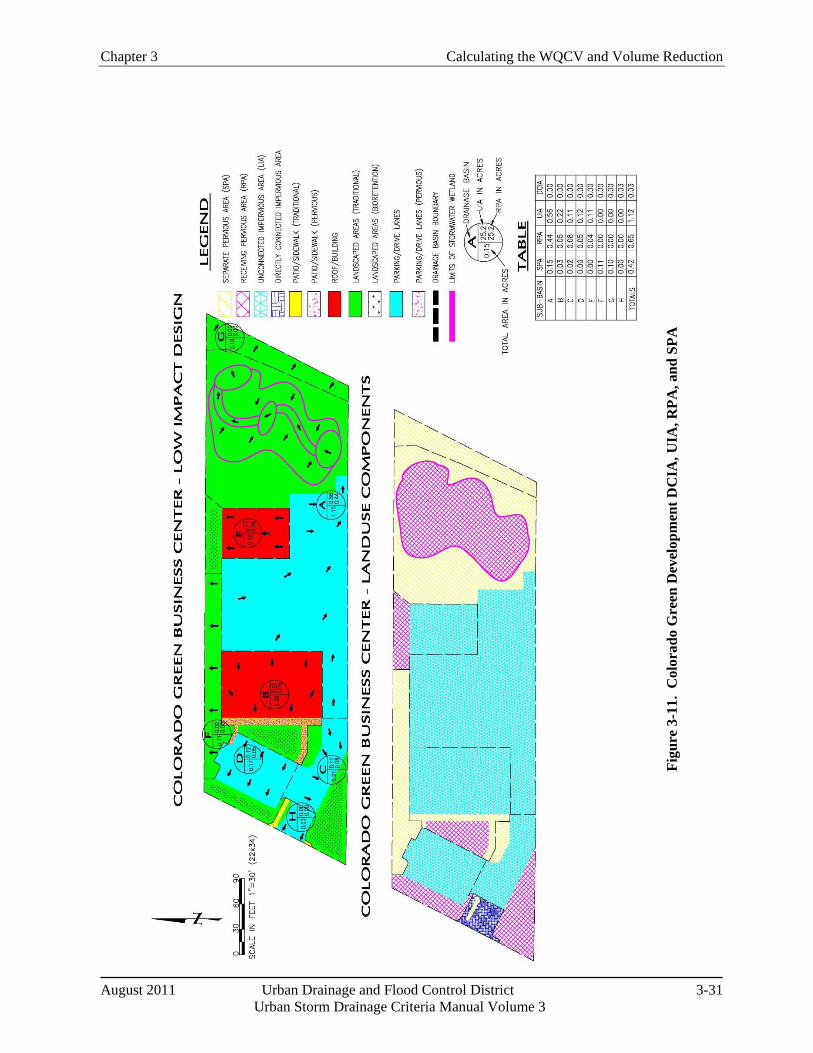
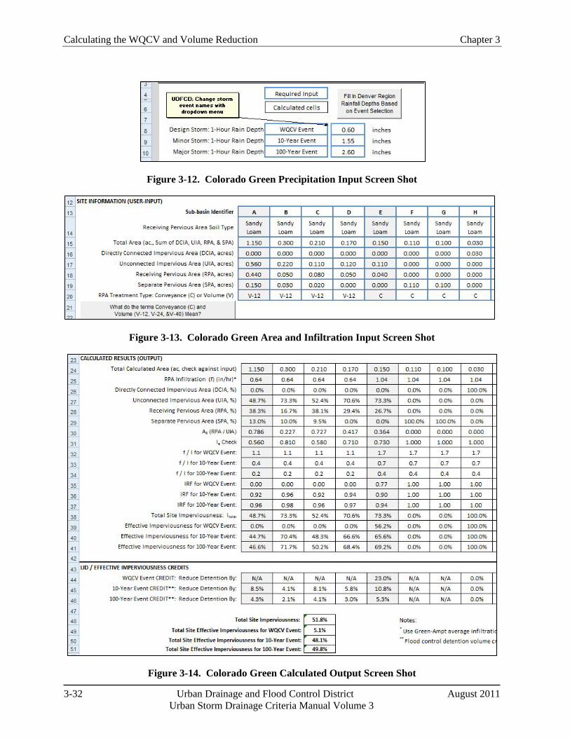
To demonstrate how the spreadsheet works, this section steps through two sub-basins from the Colorado Green development, shown in Figure 3-11. The Colorado Green development is a hypothetical LID development based on a real site plan. This example focuses on two sub-basins: (1) Sub-basin A which uses a volume-based approach and (2) Sub-basin E, which uses a conveyance-based LID approach. Note: For users working through this example using a calculator, to achieve results that closely agree with the spreadsheet entries, do not round interim results when used in subsequent equations.
Precipitation Input
Input data for precipitation include the following (see Figure 3-12).
1-hour point precipitation depth for the water quality event: The WQCV is relatively constant across the metropolitan Denver area, and is set at 0.60 inches. There is no specified duration for the WQCV, so for purposes of conservatively estimating the 1-hour point rainfall depth, the spreadsheet input assumes that the WQCV total precipitation depth occurs over a period of one hour. The spreadsheet input value for the 1-hour point rainfall depth for the water quality event should not change from the value in the example spreadsheet as long as the project is in the metropolitan Denver area.
10-year, 1-hour point rainfall depth: Determine the 10-year 1-hour point rainfall depths from Rainfall Depth-Duration-Frequency figures in the Rainfall chapter. For this example, the 10-year, 1-hour point rainfall depth is approximately 1.55 inches.
100-year, 1-hour point rainfall depth: Determine the 100-year 1-hour point rainfall depths from Rainfall Depth-Duration-Frequency figures in the Rainfall chapter. For this example, the 100-year, 1-hour point rainfall depth is approximately 2.60 inches.
Area and Infiltration Inputs
After precipitation data have been entered, the next step is to classify all areas of the site as UIA, RPA, DCIA, or SPA (see Figure 3-11) and to enter the areas into the spreadsheet in appropriate columns. Please note that blue bordered cells are designated for input, while black bordered cells are calculations performed by the spreadsheet. For the two sub-basins used in this example, A and E, inputs are:
Sub-basin A—DCIA = 0.00 ac, UIA = 0.56 ac, RPA =0.44 ac, SPA = 0.15 ac
Sub-basin E—DCIA = 0.00 ac, UIA = 0.11 ac, RPA =0.04 ac, SPA = 0.00 ac
The program calculates total area for each sub-basin as DCIA + UIA + RPA+ SPA and ensures that this value matches the user input value for total area:
Sub-basin A Total Area (ac) = 0.00 + 0.56 + 0.15 + 0.44 = 1.15 ac
Sub-basin E Total Area (ac) = 0.00 + 0.11 + 0.00 + 0.04 = 0.15 ac
Chapter 3 Calculating the WQCV and Volume Reduction
August 2011 Urban Drainage and Flood Control District 3-25 Urban Storm Drainage Criteria Manual Volume 3
The spreadsheet also calculates percentages of each of the types of areas by dividing the areas classified as DCIA, UIA, SPA and RPA by the total area of the sub-basin.
For each sub-basin, the user must enter the soil type and specify whether the RPA for each sub-basin is a conveyance-based ("C") or storage/volume-based ("V") BMP. The volume-based option should be selected only when the full WQCV is provided for the entire sub-basin. If the RPA is a volume-based BMP providing the full WQCV, the drain time must also be specified. Based on this input the spreadsheet will provide the infiltration rate. For sub-basins A and E in the example, the RPA is assumed to have sandy loam soils in the areas where BMPs will be installed. A rate of 0.64 inches per hour is used for Sub-basin A based on a sandy loam soil and a 12-hour drain time, and a rate of 1.04 inches/hour is used for Sub-basin E based on a sandy loam soil and a conveyance-based BMP type. Area and infiltration inputs are illustrated in Figure 3-13.
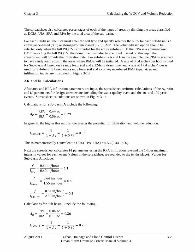
AR and f/I Calculations
After area and RPA infiltration parameters are input, the spreadsheet performs calculations of the AR ratio and f/I parameters for design storm events including the water quality event and the 10- and 100-year events. Spreadsheet calculations are shown in Figure 3-14.
Calculations for Sub-basin A include the following:
𝐴𝑅 =RPAUIA
=0.44 ac0.56 ac
= 0.79
In general, the higher this ratio is, the greater the potential for infiltration and volume reduction.
𝐼𝑎 Check = 1
1 + 𝐴𝑅=
11 + 0.79
= 0.56
This is mathematically equivalent to UIA/(RPA+UIA) = 0.56/(0.44+0.56).
Next the spreadsheet calculates f/I parameters using the RPA infiltration rate and the 1-hour maximum intensity values for each event (values in the spreadsheet are rounded to the tenths place). Values for Sub-basin A include:
𝑓𝐼𝑊𝑄
=0.64 in/hour0.60 in/hour
= 1.1
𝑓𝐼10−𝑦𝑟
=0.64 in/hour1.55 in/hour
= 0.4
𝑓𝐼100−𝑦𝑟
=0.64 in/hour2.60 in/hour
= 0.2
Calculations for Sub-basin E include the following:
𝐴𝑅 =RPAUIA
=0.04 ac0.11 ac
= 0.36
𝐼𝑎 𝐶ℎ𝑒𝑐𝑘 = 1
1 + 𝐴𝑅=
11 + 0.36
= 0.73
Calculating the WQCV and Volume Reduction Chapter 3
3-26 Urban Drainage and Flood Control District August 2011 Urban Storm Drainage Criteria Manual Volume 3
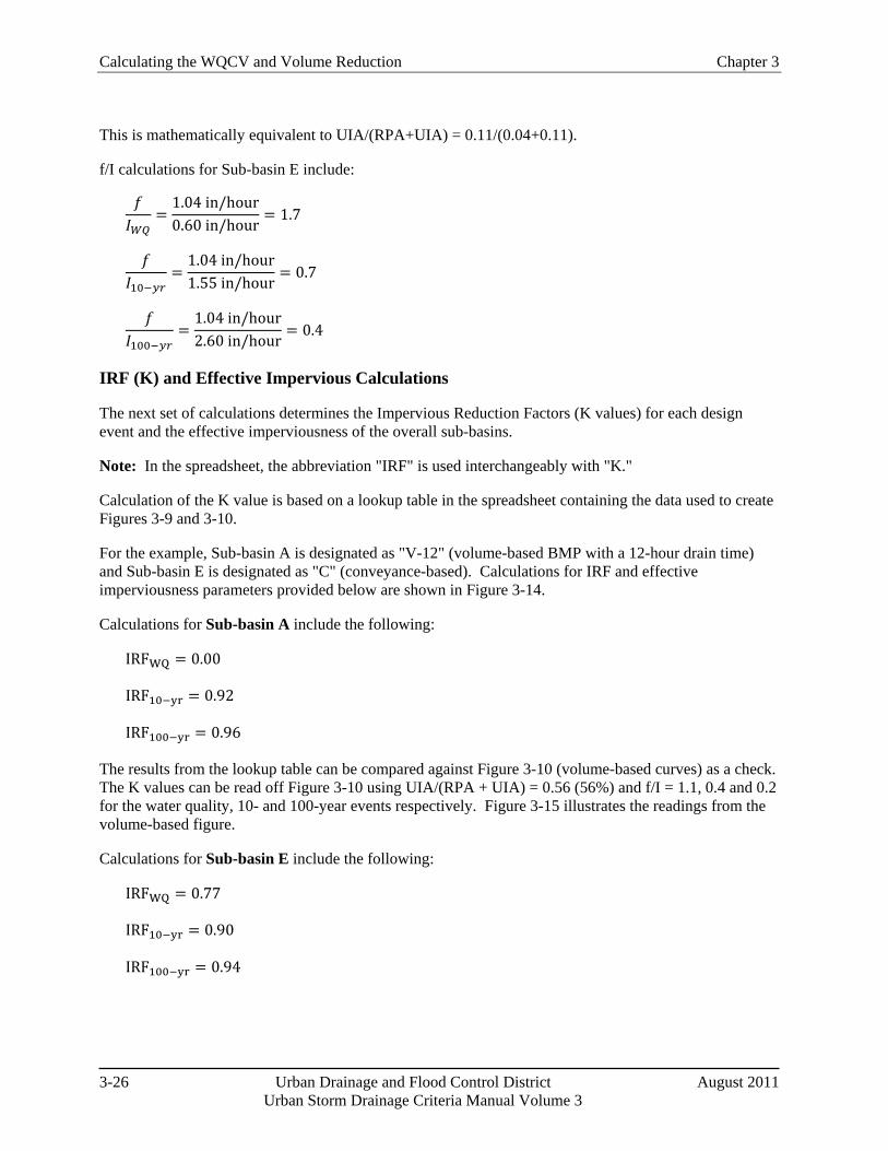
This is mathematically equivalent to UIA/(RPA+UIA) = 0.11/(0.04+0.11).
f/I calculations for Sub-basin E include:
𝑓𝐼𝑊𝑄
=1.04 in/hour0.60 in/hour
= 1.7
𝑓𝐼10−𝑦𝑟
=1.04 in/hour1.55 in/hour
= 0.7
𝑓𝐼100−𝑦𝑟
=1.04 in/hour2.60 in/hour
= 0.4
IRF (K) and Effective Impervious Calculations
The next set of calculations determines the Impervious Reduction Factors (K values) for each design event and the effective imperviousness of the overall sub-basins.
Note: In the spreadsheet, the abbreviation "IRF" is used interchangeably with "K."
Calculation of the K value is based on a lookup table in the spreadsheet containing the data used to create Figures 3-9 and 3-10.
For the example, Sub-basin A is designated as "V-12" (volume-based BMP with a 12-hour drain time) and Sub-basin E is designated as "C" (conveyance-based). Calculations for IRF and effective imperviousness parameters provided below are shown in Figure 3-14.
Calculations for Sub-basin A include the following:
IRFWQ = 0.00
IRF10−yr = 0.92
IRF100−yr = 0.96
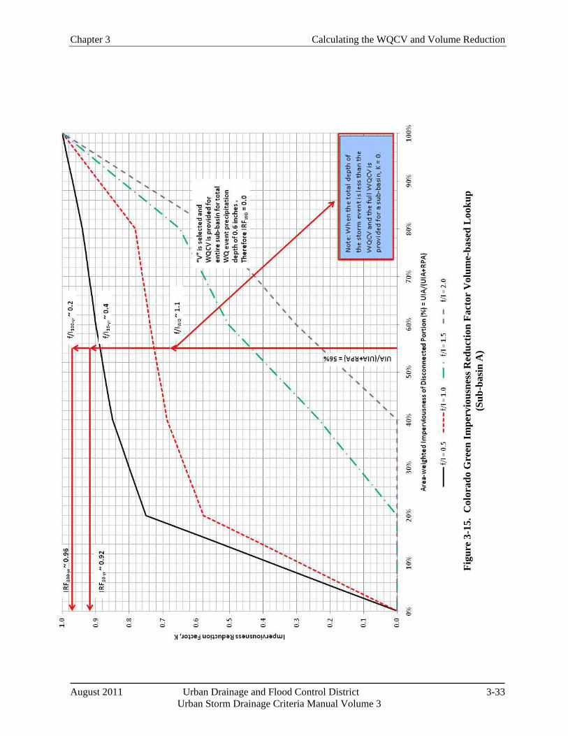
The results from the lookup table can be compared against Figure 3-10 (volume-based curves) as a check. The K values can be read off Figure 3-10 using UIA/(RPA + UIA) = 0.56 (56%) and f/I = 1.1, 0.4 and 0.2 for the water quality, 10- and 100-year events respectively. Figure 3-15 illustrates the readings from the volume-based figure.
Calculations for Sub-basin E include the following:
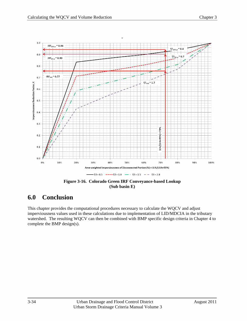
IRFWQ = 0.77
IRF10−yr = 0.90
IRF100−yr = 0.94
Chapter 3 Calculating the WQCV and Volume Reduction
August 2011 Urban Drainage and Flood Control District 3-27 Urban Storm Drainage Criteria Manual Volume 3
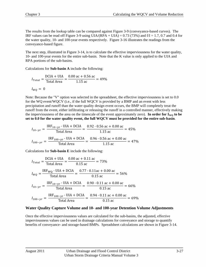
The results from the lookup table can be compared against Figure 3-9 (conveyance-based curves). The IRF values can be read off Figure 3-9 using UIA/(RPA + UIA) = 0.73 (73%) and f/I = 1.7, 0.7 and 0.4 for the water quality, 10- and 100-year events respectively. Figure 3-16 illustrates the readings from the conveyance-based figure.
The next step, illustrated in Figure 3-14, is to calculate the effective imperviousness for the water quality, 10- and 100-year events for the entire sub-basin. Note that the K value is only applied to the UIA and RPA portions of the sub-basins.
Calculations for Sub-basin A include the following:
𝐼𝑇𝑜𝑡𝑎𝑙 =DCIA + UIATotal Area
=0.00 ac + 0.56 ac
1.15 ac= 49%
𝐼𝑊𝑄 = 0
Note: Because the "V" option was selected in the spreadsheet, the effective imperviousness is set to 0.0 for the WQ event/WQCV (i.e., if the full WQCV is provided by a BMP and an event with less precipitation and runoff than the water quality design event occurs, the BMP will completely treat the runoff from the event, either infiltrating or releasing the runoff in a controlled manner, effectively making the imperviousness of the area on the timescale of the event approximately zero). In order for IWQ to be set to 0.0 for the water quality event, the full WQCV must be provided for the entire sub-basin.
𝐼10−𝑦𝑟 = IRF10−yr ∙ UIA + DCIA
Total Area=
0.92 ∙ 0.56 ac + 0.00 ac1.15 ac
= 45%
𝐼100−𝑦𝑟 = IRF100−yr ∙ UIA + DCIA
Total Area=
0.96 ∙ 0.56 ac + 0.00 ac1.15 ac
= 47%
Calculations for Sub-basin E include the following:
𝐼𝑇𝑜𝑡𝑎𝑙 =DCIA + UIATotal Area
=0.00 ac + 0.11 ac
0.15 ac= 73%
𝐼𝑊𝑄 =IRFWQ ∙ UIA + DCIA
Total Area=
0.77 ∙ 0.11ac + 0.00 ac0.15 ac
= 56%
𝐼10−𝑦𝑟 = IRF10−yr ∙ UIA + DCIA
Total Area=
0.90 ∙ 0.11 ac + 0.00 ac0.15 ac
= 66%
𝐼100−𝑦𝑟 = IRF100−yr ∙ UIA + DCIA
Total Area=
0.94 ∙ 0.11 ac + 0.00 ac0.15 ac
= 69%
Water Quality Capture Volume and 10- and 100-year Detention Volume Adjustments
Once the effective imperviousness values are calculated for the sub-basins, the adjusted, effective imperviousness values can be used in drainage calculations for conveyance and storage to quantify benefits of conveyance- and storage-based BMPs. Spreadsheet calculations are shown in Figure 3-14.
Calculating the WQCV and Volume Reduction Chapter 3
3-28 Urban Drainage and Flood Control District August 2011 Urban Storm Drainage Criteria Manual Volume 3
WQCV
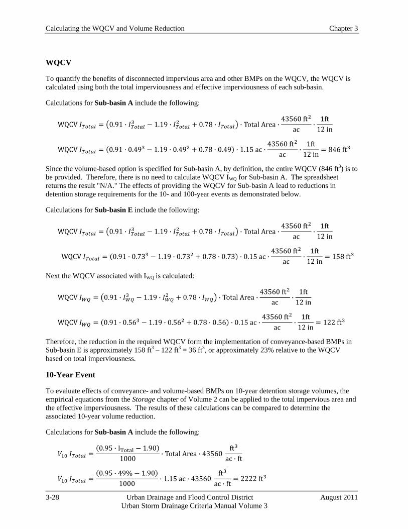
To quantify the benefits of disconnected impervious area and other BMPs on the WQCV, the WQCV is calculated using both the total imperviousness and effective imperviousness of each sub-basin.
Calculations for Sub-basin A include the following:
WQCV 𝐼𝑇𝑜𝑡𝑎𝑙 = �0.91 ∙ 𝐼𝑇𝑜𝑡𝑎𝑙3 − 1.19 ∙ 𝐼𝑇𝑜𝑡𝑎𝑙2 + 0.78 ∙ 𝐼𝑇𝑜𝑡𝑎𝑙� ∙ Total Area ∙43560 ft2
ac∙
1ft12 in
WQCV 𝐼𝑇𝑜𝑡𝑎𝑙 = (0.91 ∙ 0.493 − 1.19 ∙ 0.492 + 0.78 ∙ 0.49) ∙ 1.15 ac ∙43560 ft2
ac∙
1ft12 in
= 846 ft3
Since the volume-based option is specified for Sub-basin A, by definition, the entire WQCV (846 ft3) is to be provided. Therefore, there is no need to calculate WQCV IWQ for Sub-basin A. The spreadsheet returns the result "N/A." The effects of providing the WQCV for Sub-basin A lead to reductions in detention storage requirements for the 10- and 100-year events as demonstrated below.
Calculations for Sub-basin E include the following:
WQCV 𝐼𝑇𝑜𝑡𝑎𝑙 = �0.91 ∙ 𝐼𝑇𝑜𝑡𝑎𝑙3 − 1.19 ∙ 𝐼𝑇𝑜𝑡𝑎𝑙2 + 0.78 ∙ 𝐼𝑇𝑜𝑡𝑎𝑙� ∙ Total Area ∙43560 ft2
ac∙
1ft12 in
WQCV 𝐼𝑇𝑜𝑡𝑎𝑙 = (0.91 ∙ 0.733 − 1.19 ∙ 0.732 + 0.78 ∙ 0.73) ∙ 0.15 ac ∙43560 ft2
ac∙
1ft12 in
= 158 ft3
Next the WQCV associated with IWQ is calculated:
WQCV 𝐼𝑊𝑄 = �0.91 ∙ 𝐼𝑊𝑄3 − 1.19 ∙ 𝐼𝑊𝑄
2 + 0.78 ∙ 𝐼𝑊𝑄� ∙ Total Area ∙43560 ft2
ac∙
1ft12 in
WQCV 𝐼𝑊𝑄 = (0.91 ∙ 0.563 − 1.19 ∙ 0.562 + 0.78 ∙ 0.56) ∙ 0.15 ac ∙43560 ft2
ac∙
1ft12 in
= 122 ft3
Therefore, the reduction in the required WQCV form the implementation of conveyance-based BMPs in Sub-basin E is approximately 158 ft3 – 122 ft3 = 36 ft3, or approximately 23% relative to the WQCV based on total imperviousness.
10-Year Event
To evaluate effects of conveyance- and volume-based BMPs on 10-year detention storage volumes, the empirical equations from the Storage chapter of Volume 2 can be applied to the total impervious area and the effective imperviousness. The results of these calculations can be compared to determine the associated 10-year volume reduction.
Calculations for Sub-basin A include the following:
𝑉10 𝐼𝑇𝑜𝑡𝑎𝑙 =(0.95 ∙ ITotal − 1.90)
1000∙ Total Area ∙ 43560
ft3
ac ∙ ft
𝑉10 𝐼𝑇𝑜𝑡𝑎𝑙 =(0.95 ∙ 49% − 1.90)
1000∙ 1.15 ac ∙ 43560
ft3
ac ∙ ft= 2222 ft3
Chapter 3 Calculating the WQCV and Volume Reduction
August 2011 Urban Drainage and Flood Control District 3-29 Urban Storm Drainage Criteria Manual Volume 3
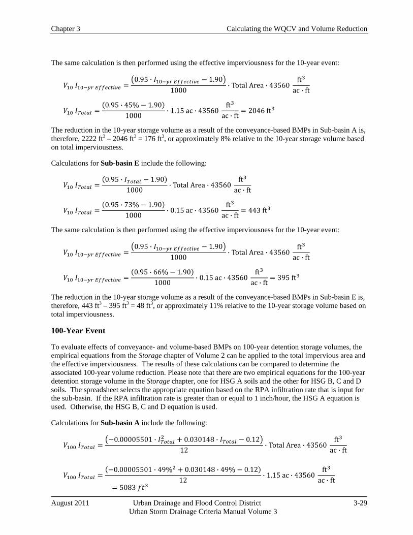
The same calculation is then performed using the effective imperviousness for the 10-year event:
𝑉10 𝐼10−𝑦𝑟 𝐸𝑓𝑓𝑒𝑐𝑡𝑖𝑣𝑒 =�0.95 ∙ 𝐼10−𝑦𝑟 𝐸𝑓𝑓𝑒𝑐𝑡𝑖𝑣𝑒 − 1.90�
1000∙ Total Area ∙ 43560
ft3
ac ∙ ft
𝑉10 𝐼𝑇𝑜𝑡𝑎𝑙 =(0.95 ∙ 45% − 1.90)
1000∙ 1.15 ac ∙ 43560
ft3
ac ∙ ft= 2046 ft3
The reduction in the 10-year storage volume as a result of the conveyance-based BMPs in Sub-basin A is, therefore, 2222 ft3 – 2046 ft3 = 176 ft3, or approximately 8% relative to the 10-year storage volume based on total imperviousness.
Calculations for Sub-basin E include the following:
𝑉10 𝐼𝑇𝑜𝑡𝑎𝑙 =(0.95 ∙ 𝐼𝑇𝑜𝑡𝑎𝑙 − 1.90)
1000∙ Total Area ∙ 43560
ft3
ac ∙ ft
𝑉10 𝐼𝑇𝑜𝑡𝑎𝑙 =(0.95 ∙ 73% − 1.90)
1000∙ 0.15 ac ∙ 43560
ft3
ac ∙ ft= 443 ft3
The same calculation is then performed using the effective imperviousness for the 10-year event:
𝑉10 𝐼10−𝑦𝑟 𝐸𝑓𝑓𝑒𝑐𝑡𝑖𝑣𝑒 =�0.95 ∙ 𝐼10−𝑦𝑟 𝐸𝑓𝑓𝑒𝑐𝑡𝑖𝑣𝑒 − 1.90�
1000∙ Total Area ∙ 43560
ft3
ac ∙ ft
𝑉10 𝐼10−𝑦𝑟 𝐸𝑓𝑓𝑒𝑐𝑡𝑖𝑣𝑒 =(0.95 ∙ 66% − 1.90)
1000∙ 0.15 ac ∙ 43560
ft3
ac ∙ ft= 395 ft3
The reduction in the 10-year storage volume as a result of the conveyance-based BMPs in Sub-basin E is, therefore, 443 ft3 – 395 ft3 = 48 ft3, or approximately 11% relative to the 10-year storage volume based on total imperviousness.
100-Year Event
To evaluate effects of conveyance- and volume-based BMPs on 100-year detention storage volumes, the empirical equations from the Storage chapter of Volume 2 can be applied to the total impervious area and the effective imperviousness. The results of these calculations can be compared to determine the associated 100-year volume reduction. Please note that there are two empirical equations for the 100-year detention storage volume in the Storage chapter, one for HSG A soils and the other for HSG B, C and D soils. The spreadsheet selects the appropriate equation based on the RPA infiltration rate that is input for the sub-basin. If the RPA infiltration rate is greater than or equal to 1 inch/hour, the HSG A equation is used. Otherwise, the HSG B, C and D equation is used.
Calculations for Sub-basin A include the following:
𝑉100 𝐼𝑇𝑜𝑡𝑎𝑙 =�−0.00005501 ∙ 𝐼𝑇𝑜𝑡𝑎𝑙2 + 0.030148 ∙ 𝐼𝑇𝑜𝑡𝑎𝑙 − 0.12�
12∙ Total Area ∙ 43560
ft3
ac ∙ ft
𝑉100 𝐼𝑇𝑜𝑡𝑎𝑙 =(−0.00005501 ∙ 49%2 + 0.030148 ∙ 49% − 0.12)
12∙ 1.15 ac ∙ 43560
ft3
ac ∙ ft= 5083 𝑓𝑡3
Calculating the WQCV and Volume Reduction Chapter 3
3-30 Urban Drainage and Flood Control District August 2011 Urban Storm Drainage Criteria Manual Volume 3
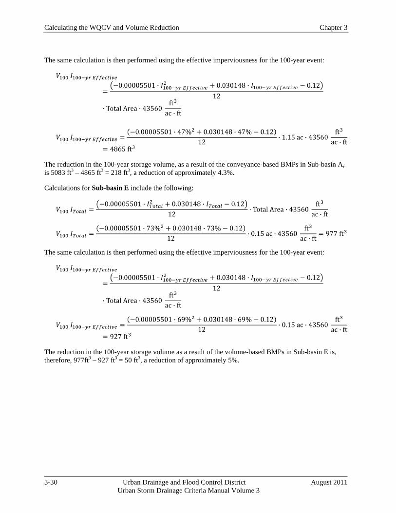
The same calculation is then performed using the effective imperviousness for the 100-year event:
𝑉100 𝐼100−𝑦𝑟 𝐸𝑓𝑓𝑒𝑐𝑡𝑖𝑣𝑒
=�−0.00005501 ∙ 𝐼100−𝑦𝑟 𝐸𝑓𝑓𝑒𝑐𝑡𝑖𝑣𝑒
2 + 0.030148 ∙ 𝐼100−𝑦𝑟 𝐸𝑓𝑓𝑒𝑐𝑡𝑖𝑣𝑒 − 0.12�12
∙ Total Area ∙ 43560 ft3
ac ∙ ft
𝑉100 𝐼100−𝑦𝑟 𝐸𝑓𝑓𝑒𝑐𝑡𝑖𝑣𝑒 =(−0.00005501 ∙ 47%2 + 0.030148 ∙ 47% − 0.12)
12∙ 1.15 ac ∙ 43560
ft3
ac ∙ ft= 4865 ft3
The reduction in the 100-year storage volume, as a result of the conveyance-based BMPs in Sub-basin A, is 5083 ft3 – 4865 ft3 = 218 ft3, a reduction of approximately 4.3%.
Calculations for Sub-basin E include the following:
𝑉100 𝐼𝑇𝑜𝑡𝑎𝑙 =�−0.00005501 ∙ 𝐼𝑇𝑜𝑡𝑎𝑙2 + 0.030148 ∙ 𝐼𝑇𝑜𝑡𝑎𝑙 − 0.12�
12∙ Total Area ∙ 43560
ft3
ac ∙ ft
𝑉100 𝐼𝑇𝑜𝑡𝑎𝑙 =(−0.00005501 ∙ 73%2 + 0.030148 ∙ 73% − 0.12)
12∙ 0.15 ac ∙ 43560
ft3
ac ∙ ft= 977 ft3
The same calculation is then performed using the effective imperviousness for the 100-year event:
𝑉100 𝐼100−𝑦𝑟 𝐸𝑓𝑓𝑒𝑐𝑡𝑖𝑣𝑒
=�−0.00005501 ∙ 𝐼100−𝑦𝑟 𝐸𝑓𝑓𝑒𝑐𝑡𝑖𝑣𝑒
2 + 0.030148 ∙ 𝐼100−𝑦𝑟 𝐸𝑓𝑓𝑒𝑐𝑡𝑖𝑣𝑒 − 0.12�12
∙ Total Area ∙ 43560 ft3
ac ∙ ft
𝑉100 𝐼100−𝑦𝑟 𝐸𝑓𝑓𝑒𝑐𝑡𝑖𝑣𝑒 =(−0.00005501 ∙ 69%2 + 0.030148 ∙ 69% − 0.12)
12∙ 0.15 ac ∙ 43560
ft3
ac ∙ ft= 927 ft3
The reduction in the 100-year storage volume as a result of the volume-based BMPs in Sub-basin E is, therefore, 977ft3 – 927 ft3 = 50 ft3, a reduction of approximately 5%.
Chapter 3 Calculating the WQCV and Volume Reduction
August 2011 Urban Drainage and Flood Control District 3-31 Urban Storm Drainage Criteria Manual Volume 3
Figu
re 3
-11.
Col
orad
o G
reen
Dev
elop
men
t DC
IA, U
IA, R
PA, a
nd S
PA
Calculating the WQCV and Volume Reduction Chapter 3
3-32 Urban Drainage and Flood Control District August 2011 Urban Storm Drainage Criteria Manual Volume 3
Figure 3-12. Colorado Green Precipitation Input Screen Shot
Figure 3-13. Colorado Green Area and Infiltration Input Screen Shot
Figure 3-14. Colorado Green Calculated Output Screen Shot
Chapter 3 Calculating the WQCV and Volume Reduction
August 2011 Urban Drainage and Flood Control District 3-33 Urban Storm Drainage Criteria Manual Volume 3
Figu
re 3
-15.
Col
orad
o G
reen
Impe
rvio
usne
ss R
educ
tion
Fact
or V
olum
e-ba
sed
Loo
kup
(Sub
-bas
in A
)
Calculating the WQCV and Volume Reduction Chapter 3
3-34 Urban Drainage and Flood Control District August 2011 Urban Storm Drainage Criteria Manual Volume 3
-
Figure 3-16. Colorado Green IRF Conveyance-based Lookup
(Sub basin E)
6.0 Conclusion This chapter provides the computational procedures necessary to calculate the WQCV and adjust imperviousness values used in these calculations due to implementation of LID/MDCIA in the tributary watershed. The resulting WQCV can then be combined with BMP specific design criteria in Chapter 4 to complete the BMP design(s).
Chapter 3 Calculating the WQCV and Volume Reduction
August 2011 Urban Drainage and Flood Control District 3-35 Urban Storm Drainage Criteria Manual Volume 3
7.0 References Driscoll, E., G. Palhegyi, E. Strecker, and P. Shelley. 1990. Analysis of Storm Event Characteristics for
Selected Rainfall Gauges Throughout the United States. Prepared for the U.S. Environmental Protection Agency (EPA). Woodward-Clyde Consultants: Oakland, CA.
Guo, James C.Y., E. G. Blackler, A. Earles, and Ken Mackenzie. Accepted 2010. Effective Imperviousness as Incentive Index for Stormwater LID Designs. Pending publication in ASCE J. of Environmental Engineering.
Guo, James C.Y. 2006. Urban Hydrology and Hydraulic Design. Water Resources Publications, LLC.: Highlands Ranch, Colorado.
Guo, James C.Y. and Ben Urbonas. 1996. Maximized Detention Volume Determined by Runoff Capture Rate. ASCE Journal of Water Resources Planning and Management, Vol. 122, No 1, January.
Urbonas, B., L. A. Roesner, and C. Y. Guo. 1996. Hydrology for Optimal Sizing of Urban Runoff Treatment Control Systems. Water Quality International. International Association for Water Quality: London, England.
Urbonas B., J. C. Y. Guo, and L. S. Tucker. 1989 updated 1990. Sizing Capture Volume for Stormwater Quality Enhancement. Flood Hazard News. Urban Drainage and Flood Control District: Denver, CO.
Water Environment Federation and American Society of Civil Engineers. 1998. Urban Runoff Quality Management. WEF Manual of Practice No. 23. ASCE Manual and Report on Engineering Practice No. 87.