chapter 2.4 data mining, analysis and modelling mining... · 2.4 – 7 data preparation no matter...

Chapter 2.4 : Data mining, analysis and modelling

2.4 – 1Author/Consultant: Dr Barry Leventhal

Chapter 2.4

Data mining, analysis and

modelling

This chapter includes:

�� What is data mining?

�� Descriptive and predictive analysis

�� The essential stages of data mining

�� The main modelling techniques

– Cluster analysis

– Regression analysis

– CHAID

– Neural networks

�� Advice to non-statisticians

�� How analysis and modelling are applied for CRM

�� Software packages

About this chapter:

Since the first edition of this Guide interest in statistical analysis and

modelling has leapt sky-high. Reasons include improvements in computing

power, reductions in costs, the growth in large databases, new analytical

theories emanating from academia, the improved education of our marketers, and

stories of its proven success.

Keeping step with these trends have been the purveyors of software packages on

which to run these new techniques.

Before you leap off into the unknown, spend a few minutes to read Barry

Leventhal’s succinct introduction to data mining. What it does. How it works. The

pros and cons of the various methods at your disposal. And, most important of

all, what the stages are in building and applying a data mining model.

2.4 – 2


But make no mistake, data mining is the future. If your organisation isn’t yet

participating, this chapter couldn’t be a better place to start.

New in this issue: This edition updates Barry’s chapter in the previous issue. It

includes new sections on data visualisation and on recent approaches to data

mining.

Dr Barry Leventhal F IDM

Head of Analysis and Modelling

Teradata, a division of NCR9 Markham Close

Borehamwood

Hertfordshire WD6 4PQ

E-mail: [email protected]

Tel: 020 8905 2634

Barry graduated in statistics at University College

London in 1971 and went on to obtain a PhD for

research into Bayesian techniques. After a period

of duty in the UCL computer centre, he began his

career at AGB in 1977. At AGB, he worked as a

statistician on continuous surveys of various

markets, including groceries and household

durables, specialising in secondary analysis of

panel data.

In 1987, Barry moved to Pinpoint Analysis, a

private sector census agency, as Head of Statistics.

His work included geodemographic analysis and

modelling projects for companies engaged in

direct marketing.

Barry moved on to Berry Consulting, a customer

management consultancy, in 1991 and spent nine

years there as Statistics Director, with

responsibility for numerous targeting and

segmentation projects.

He joined NCR in August 2000 to take up his

present post as Head of Analysis and Modelling

for Teradata in the UK.

Barry has written papers on geodemographics

and database analysis. He is a Fellow of The

Market Research Society and chairs its Census and

Geodemographics Group. He lives in

Borehamwood, Hertfordshire and likes to relax

through travel, theatre, cinema, photography and

the odd game of bridge. Since the last edition,

Barry has started to learn golf!


2.4 – 3

Chapter 2.4

Data mining, analysis and

modelling

Introduction

Sophisticated analysis of data is not exactly new to direct marketing.

Reader’s Digest, back in the early 1970s, used multiple regression analysis

on census data to predict which names on the electoral register were most

likely to respond to its magazine subscription mailings. By concentrating its

efforts on its best prospects, it saw profits increase dramatically.

Since those days, and particularly in the 1990s, many new techniques for

modelling have been developed, tested and found profitable.

Some of the techniques now in use by direct marketers are frankly very

sophisticated, and many require the attention of an experienced statistician.

This chapter, therefore, sets out to explain the basic principles of data mining,

covering analysis and modelling, as well as implementing models that you’ve built.

Then it’s over to you to pursue your interest in whatever direction you choose.

What is data mining?

Data mining sounds like it should be concerned with drilling down through seams of data,

in order to extract valuable nuggets of information, and certainly this takes place some of

the time. However, more generally, data mining is a process of discovering and interpreting

patterns in data so as to solve a business problem. This definition is deliberately broad – it

embraces sophisticated analysis and modelling applied by statisticians and also a host of

other techniques designed for a wide range of users.

For the purposes of this chapter, we will assume that the goal of data mining is to

allow an organisation to improve its marketing and sales by gaining a better

understanding of its customers. Data analysis and modelling are key stages in this

process, but are not the only stages – as we will shortly explain.

What does modelling achieve?

Modelling, in direct marketing, is often used to maximise response to a given

campaign. The fact is that in any large-scale mailing there will be names that

should not be mailed or sent a particular offer, and so on.

Basic modelling techniques in this situation can – for example by breaking down

the customer database into more and less profitable segments – select the names

that will produce the best response, or the best order value.

2.4 – 4


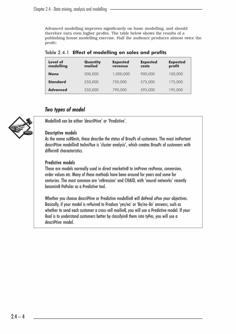
Advanced modelling improves significantly on basic modelling, and should

therefore earn even higher profits. The table below shows the results of a

publishing house modelling exercise. Half the audience produces almost twice the

profit:

Table 2.4.1 Effect of modelling on sales and profits

Level of Quantity Expected Expected Expected

modelling mailed revenue costs profit

None 500,000 1,000,000 900,000 100,000

Standard 250,000 750,000 575,000 175,000

Advanced 250,000 790,000 595,000 195,000

Two types of model

Modelling can be either ‘descriptive’ or ‘predictive’.

Descriptive models

As the name suggests, these describe the status of groups of customers. The most important

descriptive modelling technique is ‘cluster analysis’, which creates groups of customers with

differing characteristics.

Predictive models

These are models normally used in direct marketing to improve response, conversion,

order values etc. Many of these methods have been around for years and some for

centuries. The most common are ‘regression’ and CHAID, with ‘neural networks’ recently

becoming popular as a predictive tool.

Whether you choose descriptive or predictive modelling will depend upon your objectives.

Basically, if your model is required to produce ‘yes/no’ or ‘go/no-go’ answers, such as

whether to send each customer a cross-sell mailing, you will use a predictive model. If your

goal is to understand customers better by classifying them into types, you will use a

descriptive model.


2.4 – 5

The essential stages of data mining

This being a practical Guide, we shall go through a summary of all the steps in

building and applying a data mining model. These steps ought to apply to all

modelling exercises, whether basic or sophisticated.

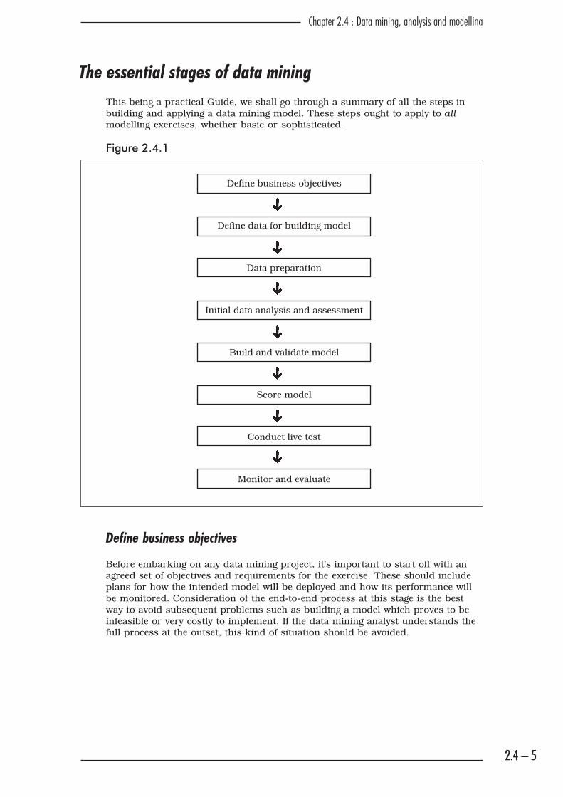
Figure 2.4.1

Define business objectives

Before embarking on any data mining project, it’s important to start off with an

agreed set of objectives and requirements for the exercise. These should include

plans for how the intended model will be deployed and how its performance will

be monitored. Consideration of the end-to-end process at this stage is the best

way to avoid subsequent problems such as building a model which proves to be

infeasible or very costly to implement. If the data mining analyst understands the

full process at the outset, this kind of situation should be avoided.

��

��

��

Define business objectives

Define data for building model

Data preparation

Initial data analysis and assessment

Build and validate model

Score model

Conduct live test

Monitor and evaluate

�

2.4 – 6


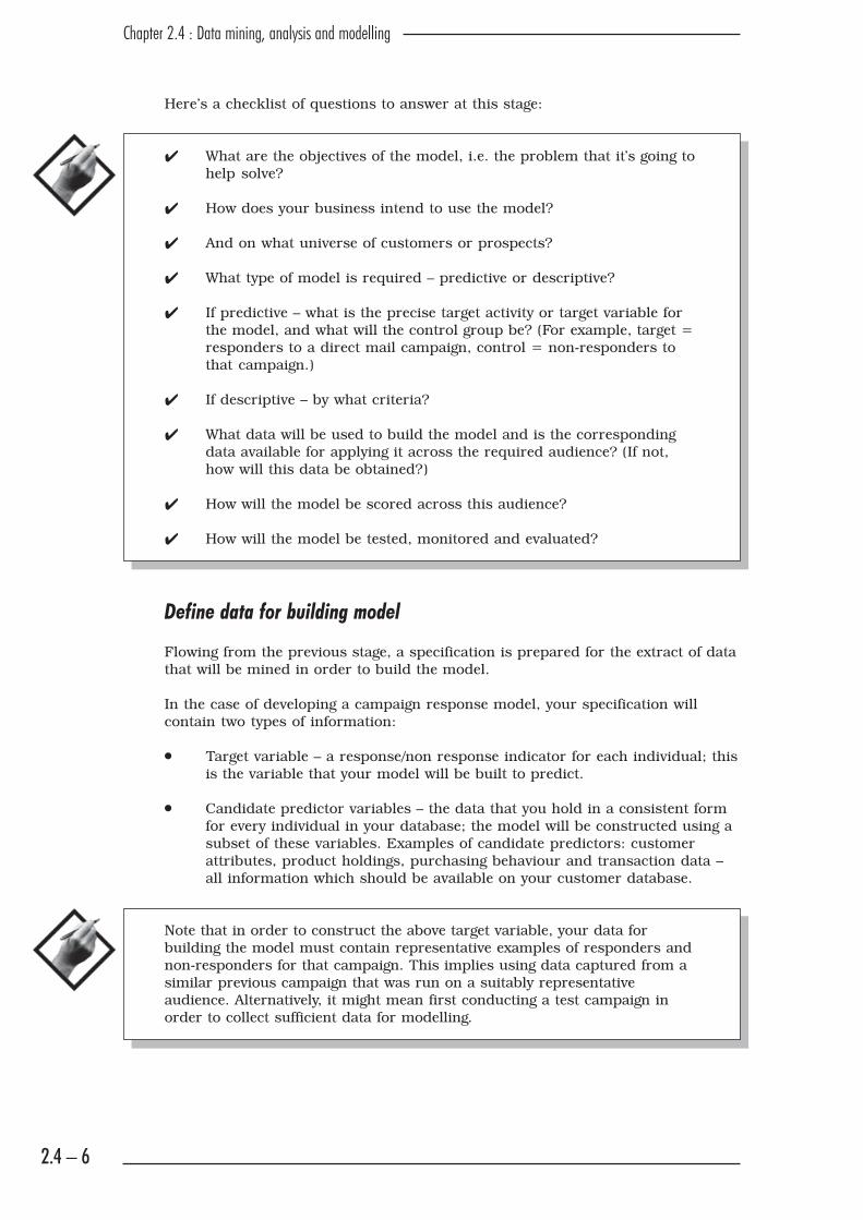
Here’s a checklist of questions to answer at this stage:

� What are the objectives of the model, i.e. the problem that it’s going to

help solve?

� How does your business intend to use the model?

� And on what universe of customers or prospects?

� What type of model is required – predictive or descriptive?

� If predictive – what is the precise target activity or target variable for

the model, and what will the control group be? (For example, target =

responders to a direct mail campaign, control = non-responders to

that campaign.)

� If descriptive – by what criteria?

� What data will be used to build the model and is the corresponding

data available for applying it across the required audience? (If not,

how will this data be obtained?)

� How will the model be scored across this audience?

� How will the model be tested, monitored and evaluated?

Define data for building model

Flowing from the previous stage, a specification is prepared for the extract of data

that will be mined in order to build the model.

In the case of developing a campaign response model, your specification will

contain two types of information:

� Target variable – a response/non response indicator for each individual; this

is the variable that your model will be built to predict.

� Candidate predictor variables – the data that you hold in a consistent form

for every individual in your database; the model will be constructed using a

subset of these variables. Examples of candidate predictors: customer

attributes, product holdings, purchasing behaviour and transaction data –

all information which should be available on your customer database.

Note that in order to construct the above target variable, your data for

building the model must contain representative examples of responders and

non-responders for that campaign. This implies using data captured from a

similar previous campaign that was run on a suitably representative

audience. Alternatively, it might mean first conducting a test campaign in

order to collect sufficient data for modelling.


2.4 – 7

Data preparation

No matter how ‘clean’ and complete the data may be, it will certainly require

preprocessing before the really interesting analysis and modelling work can

commence. Data preparation is really about converting the data into a suitable

format for the planned analytical stages, such that results will be meaningful and

not distorted by any flaws present in the original ‘raw’ data.

If the goal of the model is to predict a future behaviour, such as response to a

campaign,for which the target variable (response/non-response) is the subsequent

outcome, then all of the predictor variables should be measured at a point prior

to the campaign – ideally at the time that the mailing file was selected.

The kinds of issues that you will resolve at this stage are:

� Aggregating and merging together files in order to create a single ‘flat’ file for

analysis

� Expressing key fields, such as the ‘response/non-response’ target activity for

the model, as numeric variables

� Transforming variables into a more suitable format for analysis, e.g.

converting continuous values into sets of ranges

� Deriving new variables that may help to predict the target variable, e.g. time

since last purchase, average historic purchase frequency and value

� Dropping any fields that need to be excluded from the model, e.g. that are

poorly populated or are unreliable in some other way

� Removing outliers that could distort the model – in some cases, a group of

customers and their data may also need to be excluded, e.g. customers who

were included in the data extract, but who did not have the opportunity to

respond to the campaign in question

Initial data analysis

The first requirement in any modelling process is to summarise and

understand your data. A clear understanding of your data is imperative

before any kind of modelling can be contemplated.

The initial data analysis should take the form of identifying shapes and trends

within your data.

At this stage you will be looking at the three averages – mean, median and mode –

and at variances and standard deviations.

The data preparation and initial data analysis stages tend to be iterative and

intertwined because, until you understand the data, you will be unable to make

decisions on how to transform it in order to generate a meaningful analysis.

2.4 – 8


Data assessment

The next stage is to look much closer into your customer data, in order to find

patterns and trends. Precisely how you do this will depend upon the objectives of

the model and whether it is descriptive or predictive.

For descriptive models, you would look more closely at the variables that you are

considering using to describe customers and check how strongly they agree with

one another; the term for this is ‘correlation’. If you find that those fields are

correlated, you would decide whether to drop some of the variables from the

model or use a technique such as ‘principal components analysis’, which reduces

the data down to uncorrelated components or factors.

For predictive models, you would carry out further testing on your variables and

eliminate those which show no sign of being able to predict the target activity. In

the example of building a response model, you might compare the distribution

and mean of a variable for responders versus non-responders and look for any

signs of a different pattern. If you could see no difference between the two groups,

you might decide to drop that variable.

Build and validate model

Having prepared, assessed and understood your data, you are ready to prepare

for the modelling itself.

No matter which modelling technique you apply, it’s usually the case that you

would not wish to build a model that only works well for the particular set of

example data that you happen to be analysing. It is far more useful if the model

can also be applied to other customer data and will predict or describe customers

in the same way.

In order to check this point and avoid the mortal sin of ‘over-fitting’, you start by

selecting a random subset of your data extract for validation. You put this ‘hold-

out’ sample on one side and continue building the model with the remaining

‘development’ sample. At the end of the whole process, when you have

constructed a model that needs to be proven, you apply it to the hold-out sample

and assess the result, i.e. does the model discriminate in the same way on both

samples?

Score model

Depending upon your reasons for building the model, you may wish to apply it to

segment or make predictions for your entire customer (or prospect) base.

You may have built the model outside your database, but scoring implies either

translating the model to run directly on your database or exporting large volumes

of data to be externally scored and fed back into your database.

Either way, there are data management and IT implications inherent in scoring,

which is why I recommend that the model implementation is planned at the

outset of the project.

No matter which route you take for model scoring, it is vital that the model is

applied to precisely the same variables and calculated and transformed in exactly

the same way as when the model was built. Any minor difference in computation

of a variable will invalidate the model and may produce catastrophic results. This


2.4 – 9

can easily occur if, for example, your analyst builds the model and it is then

passed to your IT department to implement. No matter how clearly your analyst

documents the model algorithm, it can easily be misunderstood or IT can select a

different version of a variable.

The solution is to ensure that your analyst checks the results of model scoring on

a test sample provided by IT and confirms that the scores have been calculated

correctly, before the model is implemented.

Conduct live test

The first ‘live’ application of the model should be a test that can be measured and

evaluated. In the context of response modelling for direct marketing, the test

should be set up to compare model performance against a suitable control group,

such as a random sample or a selection using your existing method of targeting.

Model testing follows exactly the same approach as testing the other elements of

direct marketing and is covered in detail in chapter 4.2.

Monitor and evaluate

Assuming that your model has passed its first live test with ‘flying colours’, it

should continue to be monitored and evaluated through the use of a control group

on each execution of the campaign. This is the only way to track its performance

and detect when the time has come to update or rebuild the model.

The main modelling techniques

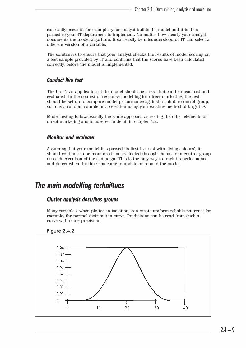
Cluster analysis describes groups

Many variables, when plotted in isolation, can create uniform reliable patterns; for

example, the normal distribution curve. Predictions can be read from such a

curve with some precision.

Figure 2.4.2

2.4 – 10


But suppose you plotted your customer base and found two peaks (nodes) on your

graph? Now you have two distinct groups to consider.

For example, if we were to plot the heights of all the people within a junior school

building, we might discover two nodes – one clustered around the average height of

the children, and one around that of their teachers.

Figure 2.4.3

We are beginning to explore the principle of clusters and this is where cluster

analysis comes into our reckoning.

In the simplified example below, we begin our analysis by creating clusters using

just two variables.

In practice, statisticians will create clusters based on several variables. If

you’re thinking of trying this, remember it can take several years of practice.

Remember also that the variables must be completely independent of each

other, i.e. not highly correlated, or they cannot be clustered.

What to do if the variables are highly correlated with one another?

There are two main options in this situation:

� Examine the variables carefully and decide which of the correlated variables

to retain in the cluster analysis and which ones to exclude. This will reduce

the variables down to a smaller set that are not highly correlated with one

another, but still describe your customers.

� Employ another technique called Principal Components Analysis (PCA) to

examine the correlations for you. PCA effectively derives a new set of scores,

known as ‘components’ or ‘factors’ that summarise the original variables, and

then the clustering is carried out on these factors.

And a final reminder: all modelling must begin with clean data, i.e. with outliers

removed.


2.4 – 11

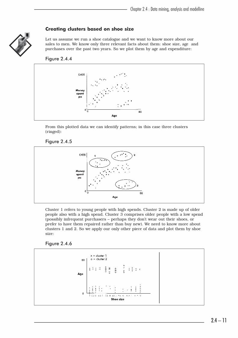
Creating clusters based on shoe size

Let us assume we run a shoe catalogue and we want to know more about our

sales to men. We know only three relevant facts about them: shoe size, age and

purchases over the past two years. So we plot them by age and expenditure:

Figure 2.4.4

From this plotted data we can identify patterns; in this case three clusters

(ringed):

Figure 2.4.5

Cluster 1 refers to young people with high spends. Cluster 2 is made up of older

people also with a high spend. Cluster 3 comprises older people with a low spend

(possibly infrequent purchasers – perhaps they don’t wear out their shoes, or

prefer to have them repaired rather than buy new). We need to know more about

clusters 1 and 2. So we apply our only other piece of data and plot them by shoe

size:

Figure 2.4.6

2.4 – 12


We see older men buying across all sizes – no clue there. But younger men are

clustered around ‘extreme’ sizes (5, 6, 11 and 12) which are difficult to find in

many shops. Perhaps we should do some research? More tests? We may have

discovered a niche market. We can now target our messages and perhaps create

special editions of our catalogue for older buyers who like the convenience of

buying from us, and for younger buyers who can’t find their sizes anywhere else.

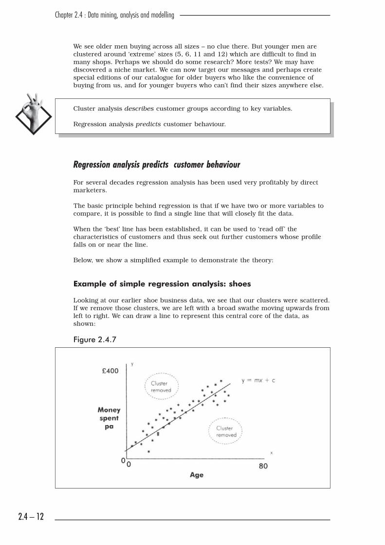
Cluster analysis describes customer groups according to key variables.

Regression analysis predicts customer behaviour.

Regression analysis predicts customer behaviour

For several decades regression analysis has been used very profitably by direct

marketers.

The basic principle behind regression is that if we have two or more variables to

compare, it is possible to find a single line that will closely fit the data.

When the ‘best’ line has been established, it can be used to ‘read off ’ the

characteristics of customers and thus seek out further customers whose profile

falls on or near the line.

Below, we show a simplified example to demonstrate the theory:

Example of simple regression analysis: shoes

Looking at our earlier shoe business data, we see that our clusters were scattered.

If we remove those clusters, we are left with a broad swathe moving upwards from

left to right. We can draw a line to represent this central core of the data, as

shown:

Figure 2.4.7


2.4 – 13

The graph above shows a clear relationship between age and money spent, i.e.

older customers spend more through this channel. As the data tends towards a

linear relationship, an equation can be created which approximately represents

the age/spend relationships as follows:

Figure 2.4.8

So, what we have done is literally ‘regress’ the individual points to a single line,

hence

‘linear regression analysis’.

We can now predict that if a man who responds is aged 30, he will spend £70 on

shoes in the next two years:

Y = (2 x 30) + 10

= 70

The most important factor in this equation is the gradient (m), because it shows

how influential the age factor is on expenditure. The gradient is often known as

the ‘weight’ or ‘score’ of x. In our example the score for age is 2.

y = mx + c

where:

y is the ��(spend)

x is the ��(age)

m is the ��, calculated from

m =yx

£120

£8020 40

eg m =120 - 80

= 240 - 20

��

C is the intercept

The intercept is where the line crosses the y-axis when x = 0

Thus, using our data:

y = 2x + 10

2.4 – 14


What if the relationship is non-linear?

Look again at the very first plot of our shoe business data and you will notice that

the relationship between age and spending is not actually a straight line (we

cheated and showed it as a straight line, in order to explain the concepts of linear

regression). How do we handle the true non-linear relationship?

In this situation, the best way to deal with non-linearity is to remove it by

applying a mathematical transformation to age, such as square root (age) or log

(age). The model is fitted using the transformed data exactly as before. In this

case, the transformation will have the effect of reducing larger ages by a greater

extent than smaller ages, and so will bring the relationship closer to a straight

line.

The single variable example above is very simplistic in its outlook and prediction

of how a customer will behave. The risk of getting the prediction wrong using this

equation is high.

To reduce the risk in regression models we add further variables. The more

variables that we add to the equation, the more accurate the final model will be,

which brings us to our next level of modelling.

Multidimensional direct marketing model

In direct marketing the dependent variable is linked to a campaign, i.e. whether a

person has, or has not, responded to a mailing. Response is normally represented

by 1 and no response represented by 0. The dependent variable could also be

actual order value or ‘likelihood-to- buy’.

Using the knowledge we have of our shoe company, we can create a response

model based upon age, shoe size and total spend in the last two years, and create

a regression model of ‘likelihood-to-respond’.

To reach the final stage of the equation we need to go through several stages, as

follows:

1. Assuming we have no response history we must first mail a random sample

of customers. During selection we must take a snapshot of their transaction

data and marketing history. This will allow us to analyse the responses once

collated. We need to know exactly what each individual customer looked like

at the time of mailing selection.

2. Once the results are available we need to compare those who responded

with those who did not, in order to discover any key differences, e.g. are

older customers more likely to respond than younger ones?

3. Experience shows that splitting continuous variables like age and income

into smaller, more discrete variables often improves the overall power of the

model. Statisticians call these split variables ‘dummy’ variables – so this we

do next. By splitting variables in this way, we ensure a greater differentiation

within each variable.


2.4 – 15

Dummy variables

Age can be split into young (18-30), middle (31-50), old (51-65) and oldest

(65+)

Total spend can be split into low (under £60), modest (£60 – £119) and high

(£120+)

Shoe size can be split into small (6 or below), usual (6.5 – 11) and large

(11.5+)

4. Now we are ready to create a regression model based upon all the split

variables. The model itself will be developed using appropriate software –

the most widely used statistical packages are mentioned towards the end of

this chapter. The skill of the statistician is to identify the best solution.

5. There are many approaches to regression modelling, but all eventually

create a set of scores for the variables in the model. Some scores are

positive, others negative. Often variables are allocated a zero score, which

implies that the variables are neither a positive nor a negative.

The final model for our shoe company mailing will look something like the

following;

Response to mailing = a x young

+ b x middle

+ c x old

+ d x oldest

+ e x low

+ f x modest

+ g x high

+ h x small

+ i x usual

+ j x large

where a to j are the scores

(Multidimensional regression is not trying to fit a best line through the data, but

the best n-dimensional plane through it. In our example it is a 10-dimensional

plane: this is impossible to either draw or imagine!)

2.4 – 16


6. A scorecard table is created to represent the model factors, for example:

Variable Score (a to j)

Age

Young -10 (a)

Middle +6 (b)

Old +12 (c)

Oldest +11 (d)

Total spend in last two years

Low -4 (e)

Modest +14 (f)

High +21 (g)

Shoe size

Small +13 (h)

Usual -10 (i)

Large +7 (j)

7. The whole mailable universe is now scored in this way. The scores for an

individual are totalled; in theory the higher a customer’s overall score, the

more likely he is to respond to the next mailing.

Example scores

Man aged 25, who has spent £90 in the past two years, and wears size 6

shoes; likelihood-to-respond score:

Age score (-10) Spend score (+14) Size score (+13) = 17

Man aged 55, who has spent £133 in the past two years, and whose shoe size

is 9; likelihood-to-respond score:

+12 +21 -10 = 23

At this point, we might surmise our best customer is a wealthy old man who

buys all his shoes from us because no one else can fit his incredibly small

feet! (If we were engaged in profiling we might be looking for more like him.)

Anyone you know?

Many years ago, in the early days of regression analysis in direct marketing,

a leading publisher regressed its customer base and discovered that its best

prospect was a man aged 38 employed at the town hall who travelled to work

on a motorcycle!


2.4 – 17

8. The next step is to test the model on another past mailing to see if what is

predicted actually happened, i.e. are the predicted scores responding as

expected?

9. If the model appears to be predicting properly, then the entire customer

base, once scored, can be segmented and a mailing programme planned

accordingly.

Modelling other dependent variables

Often direct marketers use modelling, not simply to predict response, but to

predict the actual value of an order.

Scorecards can also be used to calculate the likelihood of a customer ceasing to

respond or to buy a product. They are then known as retention models. (For an

example see the previous chapter on profiling.)

Caution!

1. We have been looking at a very basic approach to regression modelling.

Although all methods are based on the same concept, there are many other

ways of approaching the task.

2. Regression models often have a short lifespan (12 to18 months) and should

be continually reviewed and reworked. Models can be affected by economic

conditions, new product pricing, fashion changes and competitive

innovations etc.

3. Multi-variable modelling should be tackled only by a qualified statistician

using a powerful computer.

4. Scorecard regression works only when used in similar circumstances, i.e. if

developed for shoe sales it should be applied to shoe sales; for instance, if

you attempt to use the model to predict the sales of socks it is unlikely to be

useful.

CHAID: predicting response by comparing two variables

We now come to our second major predictive modelling technique: Chi-squared

Automatic Interaction Detector (CHAID).

It may sound like a Star Wars technique for spotting UFOs, and in some ways it is

– a technique for spotting patterns at speeds the human eye is unable to detect.

Decision-tree techniques are used in direct marketing to automatically segment

files into unique combinations. CHAID is the most widely used of these

techniques.

CHAID works by repeatedly splitting segments into smaller segments. At each

step it looks at a segment (or ‘cell’), considers all the variables within it, decides

which split is the most statistically reliable, and divides the cell into two smaller

cells. It then repeats the process until it decides there are no more statistically

significant splits to make.

2.4 – 18


In direct marketing we use CHAID to find the most significant factor to cause

a response or non-response. It then divides the segment into two, and

repeats the process as in the example opposite. We call the outcome a tree

diagram.

The chief advantage of CHAID is that it results in segments which are clearly

defined and easy to understand. The information it supplies can be applied

immediately; for example it can be used to make selections for direct mail as the

final cells below demonstrate.

Important:

To use CHAID, continuous data, e.g. expenditure and income, must first be

banded into categories.

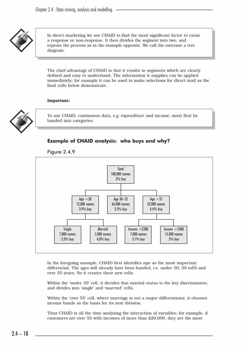
Example of CHAID analysis: who buys and why?

Figure 2.4.9

In the foregoing example, CHAID first identifies age as the most important

differential. The ages will already have been banded, i.e. under 30, 30 to55 and

over 55 years. So it creates three new cells.

Within the ‘under 30’ cell, it decides that marital status is the key discriminator,

and divides into ‘single’ and ‘married’ cells.

Within the ‘over 55’ cell, where marriage is not a major differentiator, it chooses

income bands as the basis for its next division.

Thus CHAID is all the time analysing the interaction of variables; for example, if

customers are over 55 with incomes of more than £20,000, they are the most

Total100,000 names

3% buy

Age <30 Age 30–55 Age >5512,000 names 66,000 names 22,000 names

3.9% buy 2.3% buy 4.4% buy

Single Married Income <£20K Income >£30K7,000 names 5,000 names 7,000 names 15,000 names

3.3% buy 4.8% buy 3.1% buy 5% buy


2.4 – 19

likely to buy; whereas people of the same age with lower incomes are the least

likely to buy.

If the ‘married under 30s’ were further divided by income groups, we might find

that the higher income groups produce a better response than the 5 per cent

already recorded; perhaps 6 per cent. (Caution: be sure any further division is

statistically significant.)

If we compare all the percentage response rates we can see that response from the

better segments is well over 150 per cent of that for the total mailing. We are not

only seeing how CHAID works, but also witnessing the best possible

demonstration of the power of segmentation.

(Students: you might have some fun debating which types of product might lead

to an analysis such as the one above.)

Neural networks: learning from the human brain

Another data mining technique which is gaining acceptance in direct marketing is

modelling with neural networks. Neural networks are very powerful, general-

purpose tools that can be applied for both predictive and descriptive modelling.

Neural networks were originally devised in order to explain neuron activity

within the brain and were subsequently found to be a helpful approach to

solving other problems. A neural network may be thought of simply as a

‘black box’ that processes input values to create output values.

There are several different types of neural network which broadly fall into

two groups. ‘Supervised networks’ are designed to solve prediction

problems, while ‘unsupervised’ networks are used to find clusters in data.

Neural networks are worth considering for predictive modelling when the

relationship between the inputs and the outputs is complex and highly non-linear.

I would always advocate starting off with the standard techniques, such as

regression and CHAID, in order to understand the data first and then deciding

whether a neural network model would be a useful next step. Neural networks are

more complex to set up and implement, and it is much harder to understand why

an individual record has been given a particular output value.

The latter drawback is a factor that has held back the use of neural networks for

assessing credit worthiness in financial services. If a credit application is

declined, the applicant may ask why they were ‘turned down’, but with a neural

network assessor it would be very difficult to provide the answer.

A good example of a supervised neural network application was for house value

appraisal in the US. The problem had well-understood inputs, such as size of

house, age, living space and so on, a well-understood quantified output and many

example cases where both the inputs and the output were known, i.e. previous

valuations. These examples are essential in order to train the network.

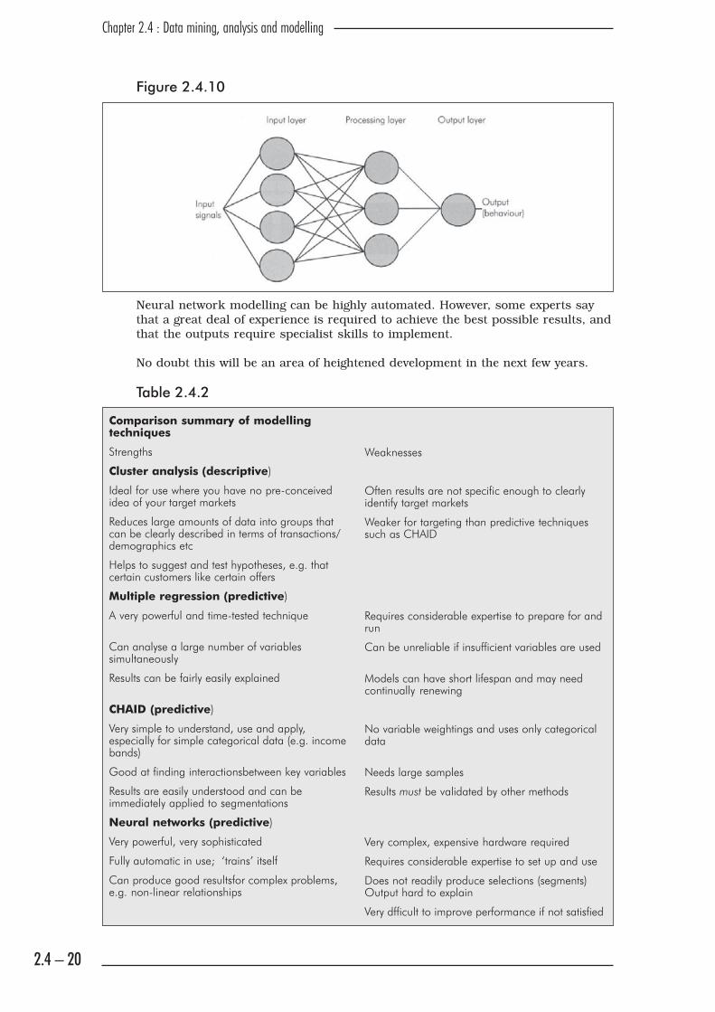
Modelling amounts to training the network to generate outputs that predict the

known outputs with sufficient accuracy. The network ‘learns’ how signals (inputs)

relate to output (response). The ‘neurons’ learn to recognise the strength and form

of each connection.

2.4 – 20


Figure 2.4.10

Neural network modelling can be highly automated. However, some experts say

that a great deal of experience is required to achieve the best possible results, and

that the outputs require specialist skills to implement.

No doubt this will be an area of heightened development in the next few years.

Table 2.4.2

Comparison summary of modelling

techniques

Strengths

Cluster analysis (descriptive)

Ideal for use where you have no pre-conceived

idea of your target markets

Reduces large amounts of data into groups that

can be clearly described in terms of transactions/

demographics etc

Helps to suggest and test hypotheses, e.g. that

certain customers like certain offers

Multiple regression (predictive)

A very powerful and time-tested technique

Can analyse a large number of variables

simultaneously

Results can be fairly easily explained

CHAID (predictive)

Very simple to understand, use and apply,

especially for simple categorical data (e.g. income

bands)

Good at finding interactionsbetween key variables

Results are easily understood and can be

immediately applied to segmentations

Neural networks (predictive)

Very powerful, very sophisticated

Fully automatic in use; ‘trains’ itself

Can produce good resultsfor complex problems,

e.g. non-linear relationships

Weaknesses

Often results are not specific enough to clearly

identify target markets

Weaker for targeting than predictive techniques

such as CHAID

Requires considerable expertise to prepare for and

run

Can be unreliable if insufficient variables are used

Models can have short lifespan and may need

continually renewing

No variable weightings and uses only categorical

data

Needs large samples

Results must be validated by other methods

Very complex, expensive hardware required

Requires considerable expertise to set up and use

Does not readily produce selections (segments)

Output hard to explain

Very dfficult to improve performance if not satisfied


2.4 – 21

Inhouse, or call in the specialists?

As a marketer, you may not be a statistician. As an entrepreneur, for example, you

may not fully understand (or have time for) the niceties of basic, let alone

advanced modelling.

For you, the aim of this chapter is, as its title suggests, primarily one of

introduction. Hopefully you are now sufficiently primed to begin talking with your

key staff, consultants and suppliers, about techniques which could easily double

your profits.

Your first decision, therefore, is whether to pursue the development of modelling

techniques yourself, e.g. inhouse, or to call in outside experts.

Here are a few more pointers that you may find helpful:

� No one modelling method, however sophisticated, is right for all

applications – but all methods, if suitable, should give broadly similar

results.

� Some software solutions are suitable only for basic applications, and some

for advanced modelling. Make sure you don’t get saddled with the latter

when what you need is the former.

� Advanced modelling can be very expensive in terms of software, systems

and skilled personnel.

� The more advanced the method, the more care and control required to

implement its conclusions.

� Once you have a model, always insist on having your model validated. This

is done by using it to predict the performance of a large set of data (i.e.

several thousand records) not used in building the model itself. If the two

outcomes correlate very closely, you have a good model.

� Some models (especially regression analysis) should be renewed at regular

intervals, e.g .12 to 18 months, if their outputs are to remain reliable.

� Remember: we’ve all heard of cases where high tech has led to high drama.

So keep it as simple as possible, learn as you go, and if in doubt, call in an

experienced statistician.

How analysis and modelling are applied for CRM

Customer relationship management (CRM) is a customer-centric process that

strives to maximise the value obtained from each customer. It aims to give each

individual the right product, at the right time, via the right channel.

Centralised data and a sound technology infrastructure are essential prerequisites

for such a goal. However, CRM also has implications for the company’s culture, its

staff and its business processes.

All of these elements are important to CRM but are outside the scope of this

chapter. However, in order to adopt a CRM strategy, you first need to understand

your customers – which, of course, is where analysis and modelling are vital.

2.4 – 22


For a start, not all customers are created equal – they will differ from one another

in terms of demographics, interests, needs, attitudes, motivations and the long-

term value that they bring to your company. So some initial cluster analysis to

segment customers can be an invaluable starting point for deciding how to

manage them.

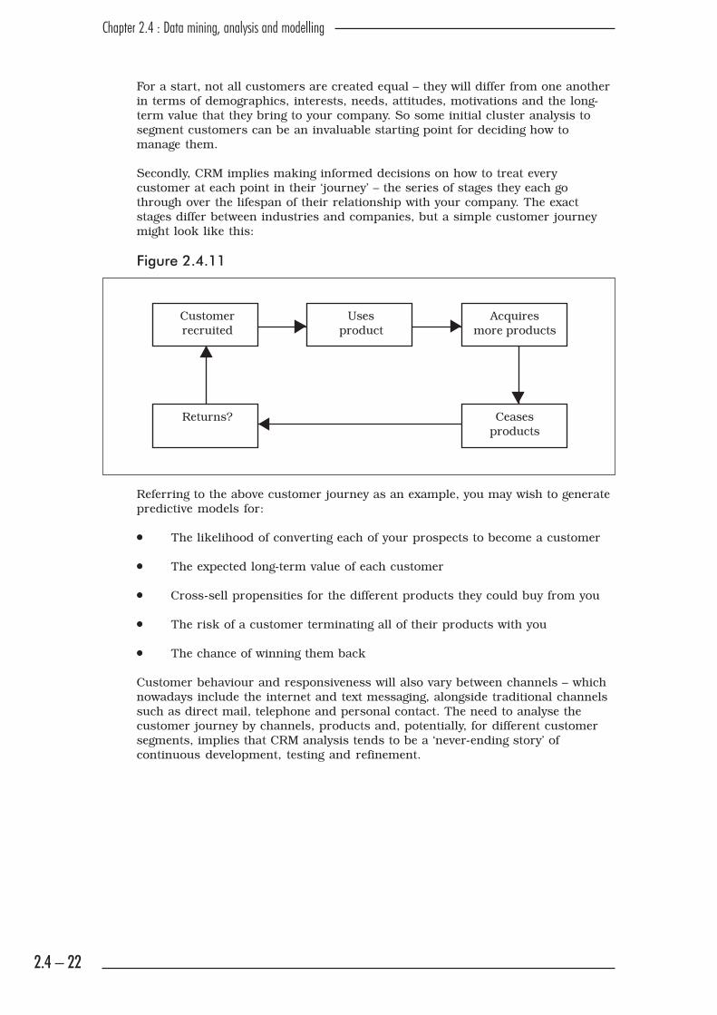
Secondly, CRM implies making informed decisions on how to treat every

customer at each point in their ‘journey’ – the series of stages they each go

through over the lifespan of their relationship with your company. The exact

stages differ between industries and companies, but a simple customer journey

might look like this:

Figure 2.4.11

Referring to the above customer journey as an example, you may wish to generate

predictive models for:

� The likelihood of converting each of your prospects to become a customer

� The expected long-term value of each customer

� Cross-sell propensities for the different products they could buy from you

� The risk of a customer terminating all of their products with you

� The chance of winning them back

Customer behaviour and responsiveness will also vary between channels – which

nowadays include the internet and text messaging, alongside traditional channels

such as direct mail, telephone and personal contact. The need to analyse the

customer journey by channels, products and, potentially, for different customer

segments, implies that CRM analysis tends to be a ‘never-ending story’ of

continuous development, testing and refinement.

Customer Uses Acquiresrecruited product more products

Returns? Ceasesproducts


2.4 – 23

Dynamic CRM analysis

CRM analysis can also be applied for ‘dynamic segmentation’, using other

advanced techniques. Two examples are:

Predictive lead generation – in Australia, the National Australia Bank

implemented a CRM model for generating sales leads. During a six-month

period, this produced over 570,000 new leads which resulted in $4.4 billion

of new business.

Internet activity – ‘e-tailers’ such as Amazon recommend books to their customers

each time they visit the website, by analysing previous purchases or titles viewed

on the site.

Data considerations

The ways in which your customer data is stored and accessed will depend upon

whether its purpose is primarily to support direct marketing or CRM.

If your main use of data is for direct marketing, you will probably wish to hold a

marketing database that stores all of the information required for targeting and

running campaigns, such as contact details, selection criteria and attributes,

products purchased and model scores. The database would also store customer

contacts and response histories.

If, on the other hand, your goal is CRM, then it becomes important to bring

together all of your databases to form a central single view of each customer. In

addition to marketing data, you would include other sources, such as payments

and arrears, service and complaints – by all channels through which you interact

with customers. Forming the ‘single customer view’ is essential for two reasons:

� Staff who interact with customers, in branches or call centres, can have

access to complete information on each relationship, thereby enabling them

to provide optimal service

� It provides a single version of the truth which avoids the possibility that

different databases in your company may be ‘out of step’ or contain

conflicting data about a customer

For example, by bringing together all data on each individual into a ‘single 360-

degree view’ and making it available throughout a retailer, the call centre operator

will have the details available about a purchase the customer recently made in

their local store. When the customer phones in with a query, the operator can

immediately provide informed advice.

2.4 – 24


Software packages for data mining, analysis and modelling

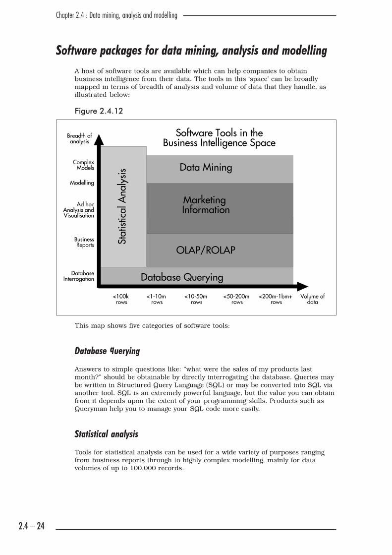
A host of software tools are available which can help companies to obtain

business intelligence from their data. The tools in this ‘space’ can be broadly

mapped in terms of breadth of analysis and volume of data that they handle, as

illustrated below:

Figure 2.4.12

This map shows five categories of software tools:

Database querying

Answers to simple questions like: “what were the sales of my products last

month?” should be obtainable by directly interrogating the database. Queries may

be written in Structured Query Language (SQL) or may be converted into SQL via

another tool. SQL is an extremely powerful language, but the value you can obtain

from it depends upon the extent of your programming skills. Products such as

Queryman help you to manage your SQL code more easily.

Statistical analysis

Tools for statistical analysis can be used for a wide variety of purposes ranging

from business reports through to highly complex modelling, mainly for data

volumes of up to 100,000 records.

Software Tools in theBusiness Intelligence Space

Breadth ofanalysis

Volume ofdata

ComplexModels

Modelling

Ad hocAnalysis andVisualisation

BusinessReports

DatabaseInterrogation

<100k rows

<1-10m rows

<10-50m rows

<50-200m rows

<200m-1bm+ rows

Data Mining

Marketing Information

OLAP/ROLAP

Database Querying

Stat

istic

al A

naly

sis


2.4 – 25

The two major suppliers used in direct marketing and CRM are SPSS and

SAS. Each has its strengths and weaknesses.

SPSS is ideal for basic users and those who prefer to work in drop-down

menu environments. Their programs run on a variety of platforms, including

PC, and they offer a reasonable level of technical support.

SAS has greater statistical and database depth and a far heavier bias to data

warehousing and system application development. They probably have the

best support desk and documentation of any software, given the number of

users worldwide. These support levels, however, reflect their complexity.

SAS is recommended for more technical users and runs on any platform

from mainframe to PC.

OLAP (Online Analytical Processing) and ROLAP (Relational OLAP)

OLAP tools operate on large databases by pre-summarising the data into

multidimensional cubes defined by key dimensions required for analysis, e.g.

products, branches, channels and geography. Users can then generate reports for

any desired subset and combination of these dimensions, a process known as

‘slicing and dicing’.

ROLAP tools achieve equivalent results within the framework of a relational

database.

Examples of software suppliers that provide OLAP or ROLAP tools are Brio,

Business Objects, Cognos and MicroStrategy. All of these can connect to a wide

range of databases that support open database connectivity (ODBC).

Marketing information

Tools for ad hoc reporting and analysis fall into this middle area of the map, and

these allow users to produce bespoke reports on customer behaviour. The four

suppliers listed under OLAP/ROLAP also provide capabilities in the area of

marketing information, with varying degrees of complexity.

Campaign management packages and CRM applications also include analytics

modules for ad hoc analysis. These packages tend to be designed for non-

technical users such as marketing managers.

Data mining

This part of the map contains data mining tools for statistical analysis and

modelling on large data volumes. Products in this area include Decisionhouse

from Quadstone, IBM Intelligent Miner, Darwin from Oracle and Teradata

Warehouse Miner from NCR. SAS and SPSS also provide data mining tools –

Enterprise Miner and Clementine, respectively.

New approaches

In recent years, some new products have been launched which focus on specific

algorithms or approaches to data mining problems. One such product is KXEN

which automates and speeds up much of the model-building process. Products

2.4 – 26


that apply ‘machine learning’ approaches are starting to appear, including

Eudaptics and GenIQ.

The issue of filling gaps in your data has also been tackled, by MOC proMISS, a

product for missing value imputation, from MOC and Atlantec Software.

Data visualisation software

Products such as Advizor (from Advizor Solutions) and seePOWER (from

Compudigm) enable dimensions and relationships in your database to be

displayed visually, and allow you to identify significant trends and patterns more

quickly by interacting with your data.

Features of data visualisation products include:

� The ability to perform high-level visualisation and then drill down into the

detail, which is essential in order to identify the cause of an abnormal

pattern of behaviour or performance

� The ability to select a subset of records for visualisation and further

analysis, by filtering of data attributes or results of previous graphical

displays

� The ability to create and publish ‘dash boards’ containing multiple graphs

on screen – these track your company’s performance; for example, customer

acquisition and retention metrics by-products and channels, so that the

information can be read and monitored by users in your organisation

� A variety of display formats, including traditional histograms, pie charts,

scatter plots and results overlaid onto geographical maps, along with

innovative techniques such as ‘heat maps’ and network connectivity graphs

chapter 2.4 data mining, analysis and modelling mining... · 2.4 – 7 data preparation no matter...

Documents