chapter 20 emergent properties in ecological systems - mcconnell biology...
TRANSCRIPT
Integrating Concepts in Biology Chapter 20: Emergent Properties of Ecological Systems
Campbell, Heyer & Paradise
December 17, 2013 Chapter 20, page 1
Chapter 20 Emergent Properties in Ecological Systems
Opening photo UN20.1 Lamar Valley, in Yellowstone National Park, where emergent properties arise
from the re-introduction of the gray wolf, a top predator.
From Yellowstone National Park (US National Park Service) website
http://www.nps.gov/archive/yell/slidefile/scenics/mvnortheast/Images/07192.jpg.
Learning Objectives
Biology Learning Objectives
1. Describe the properties of ecological systems, including food webs, indirect effects, and
nutrient cycling.
2. Evaluate how indirect effects arise through biotic interactions in ecological systems.
3. Understand how a top predator affects organisms with which it does not interact.
4. Analyze how the non-living components of ecological systems (abiota) can alter the outcome
of a biotic interaction.
5. Analyze how properties emerge from biotic interactions within ecological systems.
6. Describe how a limiting resource often results in competition.
7. Evaluate the ecological conditions that allow for species coexistence.
8. Define primary production and trophic level.
9. Explain how carbon dioxide cycles and energy from sunlight flows through an ecological
system.
10. Explain why energy transfer in ecological systems is relatively inefficient.
Bio-Math Exploration Learning Objectives
1. Predict predator and prey population dynamics by quantifying the interaction between the
two populations.
2. Calculate the overlap in resource use of competing species.
Integrating Concepts in Biology Chapter 20: Emergent Properties of Ecological Systems
Campbell, Heyer & Paradise
December 17, 2013 Chapter 20, page 2
Ethical Legal and Social Implications Learning Objectives
1. Evaluate the wider implications of re-introducing a species to an ecological system, beyond
the emergent properties and indirect effects that may arise.
2. Discuss the various ethical issues surrounding re-introduction of a predator to an area where
they may come into contact with humans or human economic interests.
3. Understand the legal issues of laws that attempt to protect endangered species, and the
implications of listing or de-listing a species.
Chapter 20 Outline
20.1 Why did more trees grow when wolves were reintroduced into Yellowstone National Park?
Bio-Math Exploration 20.1 Predicting predator and prey populations
ELSI 20.1 What are the arguments for and against species re-introductions?
20.2 What determines the outcomes of competition for a resource?
Bio-Math Exploration 20.2 How can you measure resource use overlap?
20.3 How efficient are ecological systems at transferring energy from the sun and carbon dioxide
from the air to predators?
Conclusions
You Are Here
Organizing, Big Ideas of Biology
Information Evolution Cells
Emergent
Properties Homeostasis
Levels of the
Biological
Hierarchy
Molecules 1 6 11 16 21
Cells 2 7 12 17 22
Organisms 3 8 13 18 23
Populations 4 9 14 19 24
Ecological
Systems 5 10 15 Chapter 20 25

Integrating Concepts in Biology Chapter 20: Emergent Properties of Ecological Systems
Campbell, Heyer & Paradise
December 17, 2013 Chapter 20, page 3
A hawk swoops down and catches a bird eating seeds at a birdfeeder. This is an interaction
between two individuals, a predator and its prey, but it leads to interactions between the hawk
and seed-eater populations and can cause properties to emerge in ecological systems. The
predator-prey interaction leads to energy flow in the ecosystem and affects growth of both
populations. Population growth and energy flow are emergent properties that arise because of
the actions of individuals and the coexistence of many species in ecological systems, which often
compete for limited resources. Interactions between individuals often depend upon the location
of the individuals, which may vary randomly. You cannot predict exactly where an animal will
be within an ecosystem, although you can make a reasonable guess based on its habits. The
hawk may search near feeders for potential prey. The location of an organism determines its
interactions with other organisms, populations, or ecological systems. Location leads to
flexibility in the response of ecological systems because if all the individuals in a population
were in the same place at the same time they might all get wiped out by some natural disaster or
predator. In contrast, if individuals of a species are widely distributed, it is less likely that the
entire species will die. If individual birds do not group together, predators such as hawks are
unlikely to detect every bird, and some individuals will survive. In this chapter, you will
examine emergent properties of ecological systems.
20.1 Why did more trees grow when wolves were reintroduced into Yellowstone National Park?
Context: Addition of a species into an ecological system can have unpredictable effects.
Major Themes: Biological systems exceed the sum of their parts, randomness within a
biological system provides flexibility of response, and biological systems require resources,
which results in competition or cooperation.
Bottom Line: The indirect effects of a predator on an ecological system are emergent
properties.
You will start your investigation of the emergent properties of ecological systems by looking
closely at the impact of wolves in the Yellowstone National Park ecosystem. In ecological
systems, there are predators and prey. A predator is any organism that consumes another living
organism, such that the other organism, the prey, is killed. Predators can be classified by the type
of other organism they eat, and wolves are carnivores, animals that eat other animals. Wolves
hunt in packs and eat a variety of other animals. Wolves feed mostly on large mammals, such as
deer, elk, and moose, which are all plant-eating herbivores. If more trees grow in the presence of
wolves as the Section question suggests, the wolf has effects that go beyond its direct effect as a
predator. Ecologists often construct food webs (Figure 20.1) to depict how energy flows in an
ecological system. Arrows are drawn between prey and predator, with the arrow pointed in the
direction of energy flow. Energy and nutrients, in the form of carbohydrates, proteins, and fats,
flow upward toward the predators. Organisms that are prey contain energy and nutrient
resources for predators. {Definitions: Predators are organisms that obtain energy by consuming,
and usually killing, other organisms. Prey are organisms that are consumed by predators, either
in whole or part. Food webs are diagrams that show who eats whom and how energy flows in an

Integrating Concepts in Biology Chapter 20: Emergent Properties of Ecological Systems
Campbell, Heyer & Paradise
December 17, 2013 Chapter 20, page 4
ecological system. Energy flow refers to the movement of energy-containing chemicals from
one organism to another.}
Figure 20.1 A food web. The arrows point in the
direction of the energy flow. Here plants are eaten by
grasshoppers and rodents, which are eaten by an
assortment of predators, ending in the owl and fox,
which have no predators. From
http://www.curwensville.org/146110371492860
/lib/146110371492860/f oodweb1.gif.
To understand why more trees grew when
wolves were introduced, you need to first examine
the Yellowstone National Park ecological system.
You should consider the population of wolves, the
populations of trees, and the entire ecological
system. Most of the park is more than 7,500 feet
above sea level, with forests filled with conifers,
trees with cones. There are also areas of mixed
deciduous forests, with trees that lose their leaves
each year, and grasslands. Grasslands and shrubby
plant communities predominate at lower elevations, which grade into coniferous forests at higher
elevations. Deciduous trees in this part of the world typically grow along floodplains near rivers,
but they also grow in higher elevations. Winters are very cold, and summers are mild. In
addition, wildfires are a natural part of the Yellowstone National Park ecosystems.
Integrating Questions
1. Search for information on the different abiotic conditions in forests vs. grasslands. What did
you discover? How do different conditions affect animals that live in different habitats?
Provide examples of animals that prefer to live in forests, and others that prefer to live in
open fields.
2. Search for Yellowstone National Park at the National Park Service websites (www.National
Park Service.gov and http://www.nps.gov/yell/). From what you’ve read and Yellowstone
National Park’s location (look on a map), determine the common deciduous trees that grow
in Yellowstone National Park.
3. Using the same websites, investigate the large mammals (larger than rabbits) that are
currently present in Yellowstone National Park. List the species you discovered.
4. What do the large mammals that you discovered in IQ #3 eat? Quickly sketch the species of
mammals in Yellowstone National Park along with the other species on which they feed, no
matter what type of organism they are. If you draw arrows representing the flow of energy
Integrating Concepts in Biology Chapter 20: Emergent Properties of Ecological Systems
Campbell, Heyer & Paradise
December 17, 2013 Chapter 20, page 5
and nutrients from prey to predator, you will have constructed a food web like the one in
Figure 20.1.
As European settlers expanded across most of the United States in the late 18th
and early 19th
centuries, they hunted large predators to extinction or near extinction. Within Yellowstone
National Park, the gray wolf was hunted out of existence before the National Park Service was
established to protect the natural resources. In the early days of the park, poachers routinely
hunted and logged within the boundaries of the forest. From the late 1800’s through the mid-
1920’s, hunters eliminated the gray wolf from all of the lower 48 states, with the exception of
Minnesota. Minnesota, Alaska, and much of Canada became the only refuge for the remaining
gray wolves in North America.
After wolves were eliminated, their prey faced less predation pressure. In Yellowstone
National Park, the wolves primarily eat elk, large deer-like herbivores. While an individual elk
is much larger than a wolf, an emergent property of wolves is their social behavior of hunting in
packs, which allows them to work as a coordinated unit to kill animals much larger than
themselves. Predation is an example of our theme that biological systems require resources,
which results in competition or cooperation. In this case, wolves require food resources, and
they have evolved to work cooperatively in hunting packs to acquire those resources. The social
behavior of wolves is an emergent property because you cannot predict their social behavior by
studying solitary wolves.
Integrating Questions
5. Predict the response of prey populations when populations of predators are eliminated from
an ecological system.
An emergent property of interactions between individual predators and prey is that the
populations of these species are affected. The gain in resources by a predator may provide the
energy needed for reproduction, leading to population growth. The loss of an individual in a
population of prey could affect evolution or growth rate of the population. {Connections:
Examine the effects of loss of individuals to a population in Section 24.1.} After removal of
predators such as wolves from an area, prey populations often increase in abundance very
quickly, as you may have predicted. This population boom may require the need for humans to
control the rate of growth of the prey population. One of the tasks of the National Park Service
is to monitor the populations of many species within the parks, and this is especially important
for populations such as elk that lack major predators (Figure 20.2). Elk populations had been
monitored for decades within Yellowstone National Park, and until the late 1960’s, their
populations had been managed by human hunters inside the park. Without the wolves, humans
had to limit the elk population to prevent starvation and disease. After 1968, the National Park
Service adopted a “natural regulation” strategy and no longer allowed hunting within the park.
Integrating Concepts in Biology Chapter 20: Emergent Properties of Ecological Systems
Campbell, Heyer & Paradise
December 17, 2013 Chapter 20, page 6
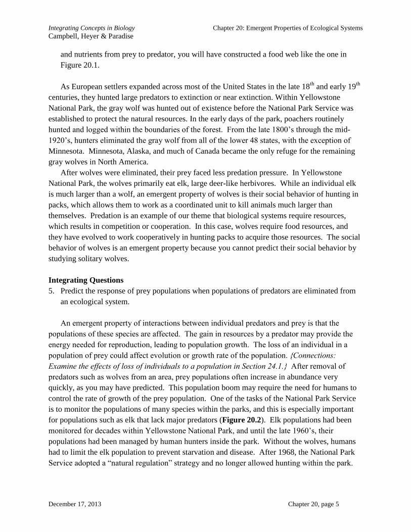
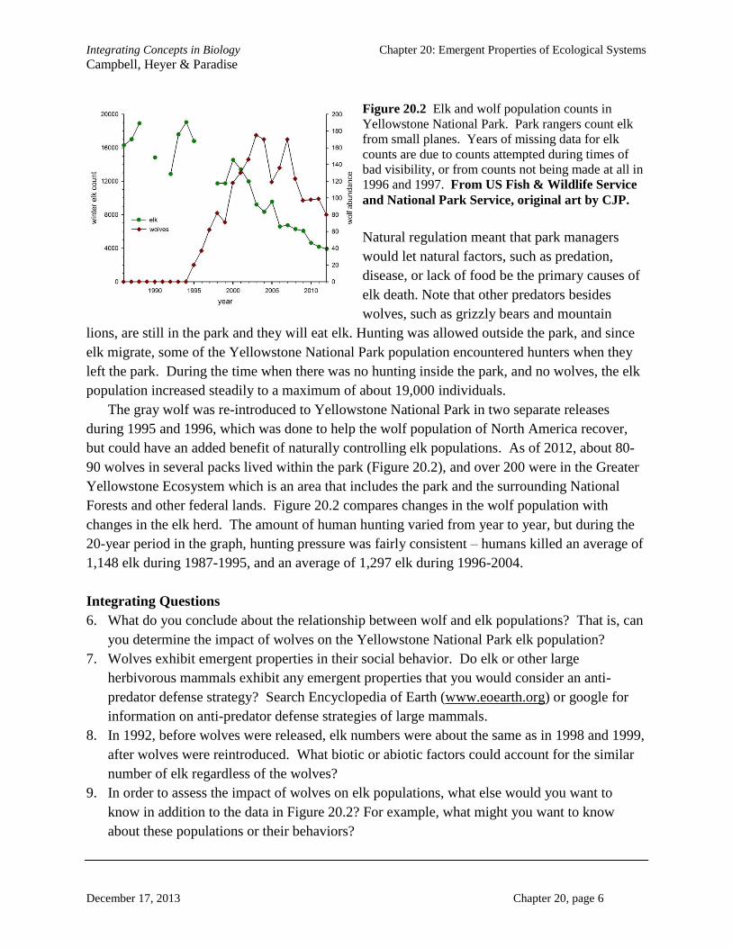
Figure 20.2 Elk and wolf population counts in
Yellowstone National Park. Park rangers count elk
from small planes. Years of missing data for elk
counts are due to counts attempted during times of
bad visibility, or from counts not being made at all in
1996 and 1997. From US Fish & Wildlife Service
and National Park Service, original art by CJP.
Natural regulation meant that park managers
would let natural factors, such as predation,
disease, or lack of food be the primary causes of
elk death. Note that other predators besides
wolves, such as grizzly bears and mountain
lions, are still in the park and they will eat elk. Hunting was allowed outside the park, and since
elk migrate, some of the Yellowstone National Park population encountered hunters when they
left the park. During the time when there was no hunting inside the park, and no wolves, the elk
population increased steadily to a maximum of about 19,000 individuals.
The gray wolf was re-introduced to Yellowstone National Park in two separate releases
during 1995 and 1996, which was done to help the wolf population of North America recover,
but could have an added benefit of naturally controlling elk populations. As of 2012, about 80-
90 wolves in several packs lived within the park (Figure 20.2), and over 200 were in the Greater
Yellowstone Ecosystem which is an area that includes the park and the surrounding National
Forests and other federal lands. Figure 20.2 compares changes in the wolf population with
changes in the elk herd. The amount of human hunting varied from year to year, but during the
20-year period in the graph, hunting pressure was fairly consistent – humans killed an average of
1,148 elk during 1987-1995, and an average of 1,297 elk during 1996-2004.
Integrating Questions
6. What do you conclude about the relationship between wolf and elk populations? That is, can
you determine the impact of wolves on the Yellowstone National Park elk population?
7. Wolves exhibit emergent properties in their social behavior. Do elk or other large
herbivorous mammals exhibit any emergent properties that you would consider an anti-
predator defense strategy? Search Encyclopedia of Earth (www.eoearth.org) or google for
information on anti-predator defense strategies of large mammals.
8. In 1992, before wolves were released, elk numbers were about the same as in 1998 and 1999,
after wolves were reintroduced. What biotic or abiotic factors could account for the similar
number of elk regardless of the wolves?
9. In order to assess the impact of wolves on elk populations, what else would you want to
know in addition to the data in Figure 20.2? For example, what might you want to know
about these populations or their behaviors?

Integrating Concepts in Biology Chapter 20: Emergent Properties of Ecological Systems
Campbell, Heyer & Paradise
December 17, 2013 Chapter 20, page 7
Bio-Math Exploration 20.1 Predicting predator and prey populations
Concept: Discrete dynamical systems to model animal populations.
Objective: Predict future elk and wolf populations.
Required Skill: Understand and manipulate logistic growth model (BME x.x).
Before making a major wildlife management decision, such as whether to introduce a new
species into an ecosystem, or how much hunting to allow, scientists and policy-makers work
together to predict the impact of the decision. Mathematical models of predator-prey interactions
can be used to help them predict outcomes. A simple model of the interaction between the gray
wolf and elk populations in Yellowstone National Park can help you see why the wolf population
decreased between 2004 and 2006, and predict what will happen to both populations over the
next several years. This predator-prey model is based on the law of mass action, the same law
that describes interactions between molecules {Connections: See BME x.x} and individuals in an
epidemic. The law of mass action states that the rate of a reaction, in this case, the rate at which
wolves kill elk, is proportional to the product of the concentrations of the reactants, in this case
the number of individuals in each population. In symbols, if we let Wt represent the wolf
population in year t, and Et represent the elk population in year t, the number of elk killed by
wolves that year should be proportional to WtEt. The increase in the wolf population due to elk
kills also should be proportional to WtEt. To complete the model, we need to make two more
assumptions:
If there were no interactions between wolves and elk, the elk population would experience
logistic growth at a rate rE {Connections: See BME 15.1} up to some carrying capacity K.
Elk are the primary food source for wolves in YNP. Therefore, if there were no interactions
between wolves and elk, the wolf population would gradually die out at rate rW.
Putting these assumptions together, the following equations allow us to make predictions
about the wolf and elk populations in year t+1, based on the populations in year t:
Et+1 = Et + rEEt(1-Et/K) – cEWtEt
Wt+1 = Wt – rWWt + cWWtEt
The carrying capacity, K, and rate constants cE and cW, in these two equations can be estimated
from population data over the last several years.
Bio-Math Exploration Integrating Questions
20.1a: Suppose there were 12,000 elk and 82 wolves in 1998. Using K=20,000, rE = 1.6, cE =
0.006, rW = 0.8 and cW = 0.000085, how many elk and wolves does the above model predict
there would be in 1999? How closely do these predictions match the actual population data

Integrating Concepts in Biology Chapter 20: Emergent Properties of Ecological Systems
Campbell, Heyer & Paradise
December 17, 2013 Chapter 20, page 8
in Figure 20.2? What might explain the discrepancy between predicted and actual
populations?
20.1b: Using the predicted 1999 elk and wolf populations from the previous question, repeat the
process to predict the populations in 2000. Again, compare the predictions to actual
populations.
The Excel file wolf-elk.xls automates the prediction process for years 1999-2020, and graphs
the predicted and actual populations on the same set of axes. Open the Excel file to check your
answers to the previous two questions, and look at the trends in the populations. How well do the
predictions track actual population sizes over this time period? How do the actual and predicted
elk population sizes differ from those predicted from logistic growth of elk in the absence of
wolves? Discrepancies between actual and predicted population sizes occur, and at least in this
instance, scientists attribute some of these changes to major environmental disturbances,
including the large fires that occurred in 1998 and a drought that occurred in the late 2000’s.
The hard part of creating a mathematical model is finding the right rate constants to match
the observed data. Once you have a model that predicts population numbers fairly accurately,
you can easily predict future population numbers. You can also estimate the potential impact of
elk hunting on both elk and wolf populations. Policy-makers and biologists need these
predictions to help them make wise wildlife management decisions.
---------------------------------------------------------------------------------------------------------------------
So far, you have considered two key species, but you have not examined the trees yet. When
wolves were absent from Yellowstone National Park, several species of trees (aspen, two species
of willows, and two species of cottonwood trees) failed to produce significant numbers of
offspring trees. The adult trees produced seeds, the seeds germinated and grew, but the seedlings
did not reach maturity.
Narrowleaf cottonwood and black cottonwood trees produce many thousands of seeds every
year. Regardless of the number of wolves, many of their seeds never become seedlings, and only
a few seedlings become mature trees. Every species evolves a reproductive strategy, which
may include such traits as age at maturity, number and survival probability of offspring, and life
span. Natural selection influences each of these traits. {Connections: Natural selection is
examined in the Big Idea of Evolution, Chapters 6-10.} A common reproductive strategy in
plants is to produce more seeds than the environment could support as mature individuals. It
might seem as if producing more seeds than a plant needs to ensure survival of one replacement
individual is a waste of resources, but there are many reasons that seeds fail to germinate and
seedlings die. Long-lived plants such as cottonwood trees that produce many seeds each year
continue to live even when a very small percentage of offspring in any one year live to maturity.
{Definition: A reproductive strategy is a suite of evolved life cycle-related traits that taken
together lead to successful existence of a species in the context of that species’ environment.}
Integrating Concepts in Biology Chapter 20: Emergent Properties of Ecological Systems
Campbell, Heyer & Paradise
December 17, 2013 Chapter 20, page 9
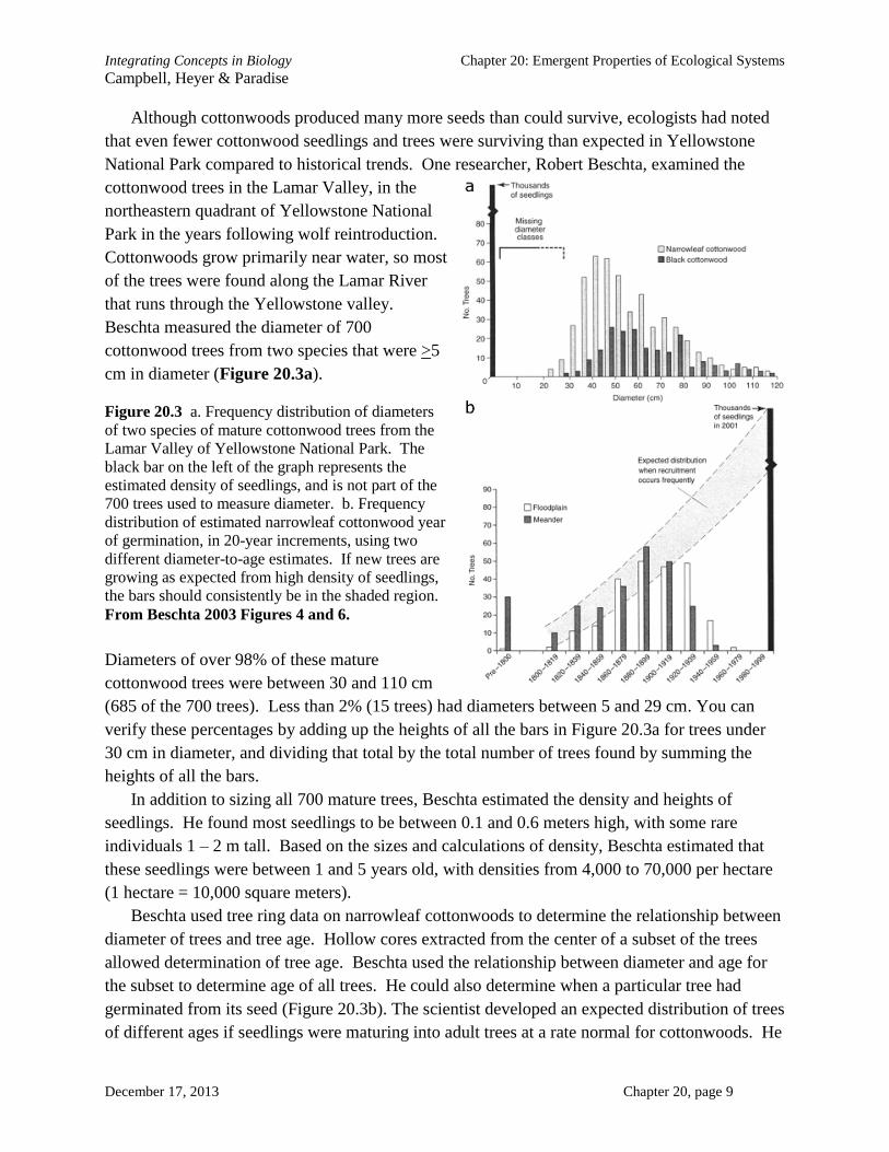
Although cottonwoods produced many more seeds than could survive, ecologists had noted
that even fewer cottonwood seedlings and trees were surviving than expected in Yellowstone
National Park compared to historical trends. One researcher, Robert Beschta, examined the
cottonwood trees in the Lamar Valley, in the
northeastern quadrant of Yellowstone National
Park in the years following wolf reintroduction.
Cottonwoods grow primarily near water, so most
of the trees were found along the Lamar River
that runs through the Yellowstone valley.
Beschta measured the diameter of 700
cottonwood trees from two species that were >5
cm in diameter (Figure 20.3a).
Figure 20.3 a. Frequency distribution of diameters
of two species of mature cottonwood trees from the
Lamar Valley of Yellowstone National Park. The
black bar on the left of the graph represents the
estimated density of seedlings, and is not part of the
700 trees used to measure diameter. b. Frequency
distribution of estimated narrowleaf cottonwood year
of germination, in 20-year increments, using two
different diameter-to-age estimates. If new trees are
growing as expected from high density of seedlings,
the bars should consistently be in the shaded region.
From Beschta 2003 Figures 4 and 6.
Diameters of over 98% of these mature
cottonwood trees were between 30 and 110 cm
(685 of the 700 trees). Less than 2% (15 trees) had diameters between 5 and 29 cm. You can
verify these percentages by adding up the heights of all the bars in Figure 20.3a for trees under
30 cm in diameter, and dividing that total by the total number of trees found by summing the
heights of all the bars.
In addition to sizing all 700 mature trees, Beschta estimated the density and heights of
seedlings. He found most seedlings to be between 0.1 and 0.6 meters high, with some rare
individuals 1 – 2 m tall. Based on the sizes and calculations of density, Beschta estimated that
these seedlings were between 1 and 5 years old, with densities from 4,000 to 70,000 per hectare
(1 hectare = 10,000 square meters).
Beschta used tree ring data on narrowleaf cottonwoods to determine the relationship between
diameter of trees and tree age. Hollow cores extracted from the center of a subset of the trees
allowed determination of tree age. Beschta used the relationship between diameter and age for
the subset to determine age of all trees. He could also determine when a particular tree had
germinated from its seed (Figure 20.3b). The scientist developed an expected distribution of trees
of different ages if seedlings were maturing into adult trees at a rate normal for cottonwoods. He
Integrating Concepts in Biology Chapter 20: Emergent Properties of Ecological Systems
Campbell, Heyer & Paradise
December 17, 2013 Chapter 20, page 10
then compared the actual and expected distributions by comparing the bars to the shaded region
in Figure 20.3b.
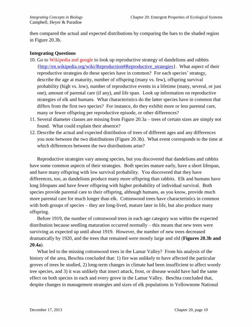
Integrating Questions
10. Go to Wikipedia and google to look up reproductive strategy of dandelions and rabbits
{http://en.wikipedia.org/wiki/Reproduction#Reproductive_strategies}. What aspect of their
reproductive strategies do these species have in common? For each species’ strategy,
describe the age at maturity, number of offspring (many vs. few), offspring survival
probability (high vs. low), number of reproductive events in a lifetime (many, several, or just
one), amount of parental care (if any), and life span. Look up information on reproductive
strategies of elk and humans. What characteristics do the latter species have in common that
differs from the first two species? For instance, do they exhibit more or less parental care,
many or fewer offspring per reproductive episode, or other differences?
11. Several diameter classes are missing from Figure 20.3a – trees of certain sizes are simply not
found. What could explain their absence?
12. Describe the actual and expected distribution of trees of different ages and any differences
you note between the two distributions (Figure 20.3b). What event corresponds to the time at
which differences between the two distributions arise?
Reproductive strategies vary among species, but you discovered that dandelions and rabbits
have some common aspects of their strategies. Both species mature early, have a short lifespan,
and have many offspring with low survival probability. You discovered that they have
differences, too, as dandelions produce many more offspring than rabbits. Elk and humans have
long lifespans and have fewer offspring with higher probability of individual survival. Both
species provide parental care to their offspring, although humans, as you know, provide much
more parental care for much longer than elk. Cottonwood trees have characteristics in common
with both groups of species – they are long-lived, mature later in life, but also produce many
offspring.
Before 1919, the number of cottonwood trees in each age category was within the expected
distribution because seedling maturation occurred normally – this means that new trees were
surviving as expected up until about 1919. However, the number of new trees decreased
dramatically by 1920, and the trees that remained were mostly large and old (Figures 20.3b and
20.4a).
What led to the missing cottonwood trees in the Lamar Valley? From his analysis of the
history of the area, Beschta concluded that: 1) fire was unlikely to have affected the particular
groves of trees he studied, 2) long-term changes in climate had been insufficient to affect woody
tree species, and 3) it was unlikely that insect attack, frost, or disease would have had the same
effect on both species in each and every grove in the Lamar Valley. Beschta concluded that,
despite changes in management strategies and sizes of elk populations in Yellowstone National

Integrating Concepts in Biology Chapter 20: Emergent Properties of Ecological Systems
Campbell, Heyer & Paradise
December 17, 2013 Chapter 20, page 11
Park, the effect of the elk browsing on cottonwood seedlings was great enough to account for the
observed gap in seed production and seedling maturation.
Figure 20.4 a. Cottonwoods in winter, with
elk herd (photo credit: Yellowstone National
Park; circa 1970s). Note the lack of small
and intermediate sized trees. b. Cottonwood
grove at Devil’s Slide refuge site along the
Yellowstone River, with a wide distribution
of tree sizes. In this site, the road on the
upslope side and the river on the downslope
side prevented elk from foraging. From
Beschta 2005 Figure 1a and 3b.
Other studies have shown heavy plant feeding by
elk on aspen and willow trees, with a similar
pattern of gaps in the frequency distribution of
ages. Beschta also studied stands of cottonwoods
where seedlings did grow to maturity (Figures
20.4b and 20.5a-c) and he found many trees in the
size ranges that were missing from the Lamar
Valley study (Figure 20.5).
Figure 20.5 Frequency distributions of narrowleaf
cottonwood (and black cottonwood in panel d)
diameters for trees >5 cm in diameter at breast height
(dbh) at five study sites in the northern Yellowstone elk
winter range. dbh is a standard measure in ecology, and
refers to diameter 1.3 meters off the ground. Note that
panel d contains the same data shown in Figure 20.3a.
From Beschta 2005 Figure 5.

Integrating Concepts in Biology Chapter 20: Emergent Properties of Ecological Systems
Campbell, Heyer & Paradise
December 17, 2013 Chapter 20, page 12
Integrating Questions
13. Summarize the major differences in the frequency distributions of cottonwood trees at the
five sites in Figure 20.5.
14. If you knew that both La Duke Spring and Devil’s Slide (Figures 20.5a and b) were bounded
on one side by a river and the other by a road, what could you conclude about factors
influencing the size distribution of cottonwood trees?
15. Beschta concluded that long-term climate change was not the reason that seedlings weren’t
maturing into trees. Compare the panels in Figure 20.5 and propose an explanation to
support his claim.
16. Beschta concluded that the loss of wolves from Yellowstone National Park probably caused
the lack of cottonwood maturation in some areas. Support his claim using data from Figures
20.2, 20.3 and 20.5.
The patterns of frequency distributions at the different sites illustrate the randomness and
variation of emergent properties, one of this Unit’s themes. Randomness and variation within
biological systems allows populations to be flexible in their response to changing environmental
conditions. Some locations of trees led to exclusion of elk, whereas others did not. The
topography of La Duke Spring and Devil’s Slide effectively excluded elk. Both sites are
bordered by a river and a road, with fairly steep slopes. While there were not many very large
trees, because the grove of trees was established after the new road was built, there were high
proportions of smaller trees present, which would not be expected if the site were frequented by
feeding elk.
The exclusion of elk allowed the narrowleaf cottonwoods to have a flexible response to the
elk-cottonwood interaction. Cottonwood populations survived in some locations where elk
cannot eat saplings, allowing long-term survival of cottonwood within the entire region, even if
some other populations may not survive. The concept of a flexible growth response by a
cottonwood population was used by Beschta to illustrate the pattern of tree growth in areas
where elk were excluded, which parallels the presence of wolves. Also, by demonstrating the
growth of young trees in elk-free areas, he was able to conclude that climate changes to the entire
ecosystem were not responsible for lack of seedling growth.
So far, you studied the elk-wolf interactions, and elk-tree interactions, but you have not
connected the wolves to the resurgence of trees within the park. You should consider all the data
to see how wolves can influence tree growth. From Figure 20.2, you determined that as wolf
numbers increased, the elk herd declined, although the correlation was far from perfect.
However, you also know that tree maturation was low even when humans restricted the size of
elk herds through hunting and relocation programs that occurred from the 1920’s through the
1960’s. It was not until after the “natural regulation” of 1968 began that elk populations reach
their highest levels. Yet narrowleaf cottonwood sapling growth is absent throughout much of the
Lamar Valley from 1920 to the mid-1990’s, which indicates the number of elk is not the only
determining factor for tree survival. The wolf was the only component of the ecological system

Integrating Concepts in Biology Chapter 20: Emergent Properties of Ecological Systems
Campbell, Heyer & Paradise
December 17, 2013 Chapter 20, page 13
missing during that time period. What is the difference between when humans controlled elk
population (1926 – 1968) and when wolves controlled elk populations (mid-1990s and on)?
When a group of scientists tried to determine the difference between human and wolf
regulation of elks, they initially focused on the direct effects of wolf predation. However,
predation did not sufficiently answer the question about the re-emergence of aspen, willow, and
cottonwood trees. If the number of elk killed was the only factor that determined the success of
trees, then human control would have yielded similar results to the natural control. They
reasoned that indirect effects of predation might be the key to understanding the emergent
property of tree survival in the presence of wolves. Indirect effects are another emergent
property of ecological systems.
Once wolves were reintroduced to Yellowstone National Park, elk had to face a predator that
they had not encountered in many decades, and certainly no elk living in the park in 1995 had
ever confronted a pack of hungry wolves. The elk that survived this new predation threat would
be the individuals that were more vigilant for these predators. Are there any costs to the
surviving elk with increased vigilance? You will see how investigators collected some of the
data to answer this question. {Definition: Indirect effects in ecological systems are effects of
one species on other species mediated through shared interactions with a third species or group
of species.}
Scott Creel and his colleagues used radiotracking to study the locations of 14 elk that were
part of herds living in Gallatin Canyon, during 2002 and 2003. Radiotracking is a method in
which scientists fit individual members of a population with collars that transmit a radio signal.
The scientists pick up the radio signal with receivers, which they used to determine their
locations. Creel and his colleagues also tracked wolves in two out of three packs that used the
same geographic area. The scientists assessed the habitat use of elk during times when wolves
were present and when wolves were not detected in the area of the herd (Figures 20.6). When
these data, which are from just one area the scientists studied, are put into a computer model with
all their other data to predict habitat use when wolves are present or not detected, they were able
to estimate the probability of grassy
areas or forest occurring where elk
are located (Figure 20.7).
Figure 20.6 Radiotracked elk locations
and elk kills in Gallatin Canyon within
the Greater Yellowstone Ecosystem
(outside of Yellowstone National Park).
Locations were in conifer forests, the
edge between forest and open grass, and
open grass habitat. Wolves were either
detected nearby or not when each elk
observation was made. Data from Creel
et al. 2005, Figures 1a and b, original
art by CJP.

Integrating Concepts in Biology Chapter 20: Emergent Properties of Ecological Systems
Campbell, Heyer & Paradise
December 17, 2013 Chapter 20, page 14
Figure 20.7 Effects of wolf presence on habitat
use by elk. The probabilities shown are the
probabilities that grassy areas or coniferous areas
were prevalent where elk were found. Bars show
means and 95% confidence intervals. From
Creel et al. 2005 Figure 3, original art by CJP.
Integrating Questions
17. What do the data in Figure 20.6 tell you
about the location of elk kills and the location
of elk when wolves were known to be nearby
or not detected?
18. What are your conclusions from this graph regarding habitat use of elk when wolves are
present or not detected?
19. What is the difference between wolves being “not detected” and being “absent?” The
scientists performing this study were clear in the use of the phrase “wolves were not
detected.” What are the possible implications of this distinction for elk behavior and
increasing the variability in the data set?
Creel and his colleagues concluded that the elk alter their habitat use when they detect the
presence of wolves. From Figures 20.6 and 20.7, you see that the elk behavior is not perfectly
correlated with the presence of wolves – there is variation in elk behavior. Elk are not perfect in
their detection of wolves, nor are they perfect in selecting habitats based on their assessment of
the risk of predation. Furthermore, the scientists had not placed a radio transmitter on every wolf,
and so some could be in the area without detection. Elk cannot know where every wolf is, nor
do they know the best place to avoid detection by their predators – if they did, wolves would
starve for lack of prey. In addition, prey animals often assess their risk not only on the presence
of predators, but also on their need for food. For instance, a hungry elk might take more chances
on feeding in the grassy areas, where their preferred food is, than an elk with a full belly that
may remain in the relative safety of the conifer forest.
The scientists concluded that elk move in response to the presence of predators within 1
kilometer of their location. Again, variability in elk movements results from variability in wolf
detection by elk. Elk are more likely to occupy sites, such as grassy areas, where they can forage
with confidence that wolves are absent (that is, they haven’t detected them). Conversely, elk are
more likely to seek protective cover in coniferous forests when they detect wolves nearby.
Altering habitat preference based on the presence of wolves is likely to have several effects,
including a decrease in the energetic resources obtained by elk (not eating grass all the time), an
increase in energetic costs by elk (more vigilance when eating grass), and a possible release of
herbivore pressure on tree seedlings (fewer elk feeding in the grass where new seedlings could

Integrating Concepts in Biology Chapter 20: Emergent Properties of Ecological Systems
Campbell, Heyer & Paradise
December 17, 2013 Chapter 20, page 15
sprout). Recall that the grassy areas are often at lower elevations, in flood plains or near rivers,
and this is exactly where the groves of cottonwood, aspen, and willows are often located.
Now that you have made a connection between trees, elk and wolves, it would be wise to
determine if any other factors influence where the elk eat and indirectly what they eat. To
determine whether the changes in elk behavior that occur in the presence of wolves have an
indirect effect on tree growth, you would need to know whether more trees like cottonwood,
aspen and willow are growing in areas where elk are spending less time. In another study,
Beschta and a colleague, William Ripple, measured stands of aspen trees in elevated and
floodplain sites. Like the cottonwoods, there are gaps in the growth of aspen forests that
correspond to the time when wolves were absent from the park (see Figures 20.3 and 20.5). The
scientists determined the recent history of browsing and measured the height of the five tallest
young aspen in each of several stands. They estimated the annual heights of these trees for the
nine previous years based on the
pattern of browsing damage of the
highest branches (Figure 20.8).
Figure 20.8 Comparison of terrain on
tree growth. a. Percentage of leading
shoots of aspen eaten. b. Average
aspen height. From Ripple and
Beschta 2007 Figures 1c and d.
At each tree they also measured the
number of downed large logs that
were within 3 meters of the tree
because logs might impede elk
escaping through the forest. The
scientists hypothesized that aspen
trees would be taller nearer streams
than in upland areas if wolves are
frequenting upland areas. Aspens also were predicted to be taller at sites with downed logs than
sites with fewer or no downed logs due to behavior modification of the elk caused by the
reintroduction of wolves. Of four habitat types studied, they predicted that stream-side sites with
logs would have the highest predation risk, whereas upland sites without logs would have the
lowest predation risk. Elk might be able to assess the risk of predation in different habitats, and
predation risk on elk should then correlate with aspen growth (Figure 20.8).
Integrating Questions
20. Restate the predictions of Ripple and Beschta regarding aspen tree height and elk foraging, as
they relate to predation risk on elk. If the foraging pattern of elk relates to their perceived
predation risk, such that they forage less in areas where they perceive more risk, then

Integrating Concepts in Biology Chapter 20: Emergent Properties of Ecological Systems
Campbell, Heyer & Paradise
December 17, 2013 Chapter 20, page 16
according to Figure 20.8, which habitat has the highest predation risk? Does your conclusion
match the predictions of the scientists?
21. What is the effect of downed logs on predation risk? Compare the general effect of logs
within a habitat from Figure 20.8: upland with logs vs. upland without logs, and stream-side
with logs vs. stream-side without logs. Then compare the two uplands curves with and
without logs vs. the two stream-side curves with and without logs. Is the effect of logs
within a site greater than or less than the effect of habitat type?
It is uncommon for a policy change to be measured so carefully to determine whether the
policy was a success or not. Many scientists studying Yellowstone National Park ecological
system concluded that the regrowth of the vegetation was likely due to a combination of altered
elk behavior and reduced elk numbers in response to the reintroduction of wolves. Much of the
regrowth occurred near rivers, which wolves frequently use, and would thus present a high
predation risk to the elk. Aspen stands with downed logs would present a further risk of
predation as areas with lots of downed logs would be difficult to run through while escaping
wolves.
The change in elk behavior leads to indirect responses throughout the system, due to
emergent properties. As aspen, willow and cottonwood regenerate and begin reproducing again,
other aspects of ecological systems are predicted to change. Beschta and Ripple analyzed the
communities of berry-producing shrubs that often grow under aspen trees (Figure 20.9). Among
other things, they examined the relationship between shrub height and aspen height and the
number of different species of shrubs under aspen stands that were classified into different height
classes – some stands contained many small aspens, others had aspens that were taller than what
elk could usually reach and browse upon, as discussed for Figure 20.8.
Figure 20.9 Effects of
aspen regrowth on shrubs.
a. Statistically significant
regressions of berry-
producing shrub height vs.
understory aspen height. b.
Average number of berry-
producing shrub species in
aspen stands (±95%
confidence intervals) in
three height categories.
From Beschta and
Ripple 2012 Figures 3
and 4.
Integrating Concepts in Biology Chapter 20: Emergent Properties of Ecological Systems
Campbell, Heyer & Paradise
December 17, 2013 Chapter 20, page 17
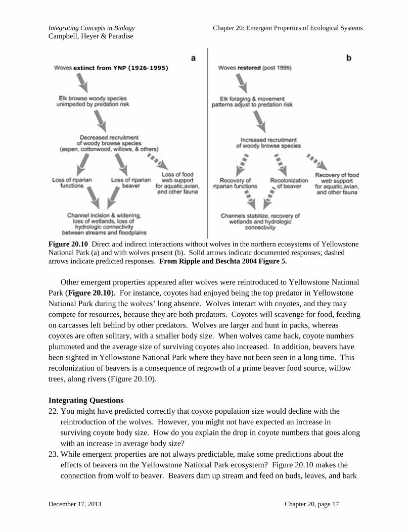
Figure 20.10 Direct and indirect interactions without wolves in the northern ecosystems of Yellowstone
National Park (a) and with wolves present (b). Solid arrows indicate documented responses; dashed
arrows indicate predicted responses. From Ripple and Beschta 2004 Figure 5.
Other emergent properties appeared after wolves were reintroduced to Yellowstone National
Park (Figure 20.10). For instance, coyotes had enjoyed being the top predator in Yellowstone
National Park during the wolves’ long absence. Wolves interact with coyotes, and they may
compete for resources, because they are both predators. Coyotes will scavenge for food, feeding
on carcasses left behind by other predators. Wolves are larger and hunt in packs, whereas
coyotes are often solitary, with a smaller body size. When wolves came back, coyote numbers
plummeted and the average size of surviving coyotes also increased. In addition, beavers have
been sighted in Yellowstone National Park where they have not been seen in a long time. This
recolonization of beavers is a consequence of regrowth of a prime beaver food source, willow
trees, along rivers (Figure 20.10).
Integrating Questions
22. You might have predicted correctly that coyote population size would decline with the
reintroduction of the wolves. However, you might not have expected an increase in
surviving coyote body size. How do you explain the drop in coyote numbers that goes along
with an increase in average body size?
23. While emergent properties are not always predictable, make some predictions about the
effects of beavers on the Yellowstone National Park ecosystem? Figure 20.10 makes the
connection from wolf to beaver. Beavers dam up stream and feed on buds, leaves, and bark
Integrating Concepts in Biology Chapter 20: Emergent Properties of Ecological Systems
Campbell, Heyer & Paradise
December 17, 2013 Chapter 20, page 18
of trees, so you might be able to predict further changes to this ecological system. For
instance, what would be an emergent property associated with increased beaver feeding and
habitat alteration due to new beaver dams?
You know that biological systems, from wolves, to elk, to beaver, require resources. In order
to obtain their resources, wolves hunt cooperatively in packs, although different packs must
compete for territory. Elk have to maintain vigilance in order to avoid predation while foraging
for the food they need; as they alter their behavior to reduce the risk of predation, they may
exhibit a trade-off. Here, elk exchange abundant food consumption for increased survival.
{Definition: A trade-off is a compromise that occurs as organisms exchange one behavior or
resource for another.}
The entire ecological system responded to the presence of wolves in ways that no one
predicted when wolves were reintroduced to the park. Beaver were not present in the park for
many years in part because their preferred trees (young willow trees) were not present in high
abundance; the number of beaver colonies went from one to 12 between 1999 and 2010. The
ecological system contained within Yellowstone National Park exceeds the sum of the individual
species living in the park.
The randomness of this large ecological system provides flexibility of response. For
instance, the locations of downed logs, the meandering of a river, or the movements of a herd of
elk and a pack of wolves, may all play a role in whether a cottonwood or aspen can grow to
maturity. Depending on the abiotic conditions at a particular location such as an upland area or a
floodplain, trees may or may not grow regardless of the elk. The carcasses left behind by wolves
provide a bounty to other scavengers, including coyotes, which may explain the larger sizes of
individual surviving coyotes that were not killed due to resource competition with wolves. There
may be more variability of response among scavengers depending on abundance and location of
the resource, possibly leading to more competitive interactions as scavengers attempt to gain
these resources. You have learned how the interactions between predators and their prey can lead
to emergent properties. In the next section, you will examine how emergent properties arise
from competitive interactions.
Ethical, Legal, and Social Implications Box 20.1
What are the arguments for and against species re-introductions?
Over the last several decades, many species have disappeared throughout all or part of their
original ranges. The most common reasons for loss of species are habitat loss, pollution,
competition with invasive species and global climate change, all primarily caused by human
overpopulation and overconsumption of resources. Many people argue that to restore ecological
systems humans must reintroduce species to their natural ranges, assuming they still exist
somewhere. Perhaps the most successful case of a species that was restored to its habitat is the
California condor, with the largest wing span of any bird (9 feet). All 22 of the remaining
Integrating Concepts in Biology Chapter 20: Emergent Properties of Ecological Systems
Campbell, Heyer & Paradise
December 17, 2013 Chapter 20, page 19
condors were captured in 1987 and placed into a captive breeding program with the intent to re-
release them into the wild. Since 1991, over 150 young adults have been released and 150 are
still in the breeding program. Other species, such as gray wolves, may require some assistance
from humans to expand back into their original ranges.
Reintroducing the gray wolf to Yellowstone National Park was the result of a long debate
over the value of reintroducing a predator. Wolves have been reintroduced in other places, and
similar debates have occurred in these places, too, including Scandinavia and the Adirondack
Park in New York State. In addition to the biological data required to make a successful
reintroduction, social scientists conducted many surveys of public attitudes and perceptions
towards wolf reintroductions. While 60% of the general population supports reintroduction, only
35% of ranchers do. As you might imagine, ranchers were nervous and opposed to the idea,
fearing for their livestock. While a majority of the general population has a positive attitude
towards wolves, more of those people live in urban areas and have little or no experience with
wolves. People who have a negative attitude towards wolves live near the wolves. Others argue
against reintroduction for other reasons, saying that money spent on captive breeding and
reintroduction would be better spent solving societal problems, like homelessness and poverty.
As you consider these arguments, you can appreciate the complexities of conservation.
Because humans eliminated top predators, do we now have an ethical obligation to restore those
species to their former ranges? When predators were eliminated, not much was known of the
ecological roles of those species. The direct and indirect roles of wolves have been demonstrated
in their return to Yellowstone National Park. Gray wolves were the only native vertebrate
species that was not still present in Yellowstone prior to its reintroduction. However, local
residents are concerned about loss of life or economic damage to crops or livestock that may
result from wolf reintroduction. Humans eradicated gray wolves from the park and the
surrounding area because they perceived the wolves as a threat to livestock and family, and that
perception persists. Should federal tax dollars be used to conduct additional research to
determine whether these perceived threats were justified or not?
Ethicists have argued that if we honor our ethical duty to a past ecosystem by reintroducing a
missing species, then we create a new conflict with our ethical duties to present and future
ecosystems, in that a missing species may cause harm to other species. “Do our duties to existing
ecosystems outweigh our duty to past ecosystems?” If we reintroduce a species to an area where
it is no longer present, species that currently thrive there may be harmed. In the case of wolves,
prey populations were harmed, but some species increased in abundance after reintroduction. As
you know, indirect effects and emergent properties are difficult to predict. How can you weigh
these possible outcomes when you can’t even predict them?
Finally, there is a concern among ecologists that a plan by humans to “restore” an ecosystem
leads the public to believe that ecosystems are naturally static. Ecological systems are naturally
dynamic, and constantly undergo changes. Extinction of a species can be caused by non-human
processes, and if humans are perceived as a natural part of an ecosystem, then humans are just
another natural cause of extinction, as natural as an ice age or a volcano. Thus, both
Integrating Concepts in Biology Chapter 20: Emergent Properties of Ecological Systems
Campbell, Heyer & Paradise
December 17, 2013 Chapter 20, page 20
reintroductions and eliminations may be viewed as equally harmful or beneficial to ecological
systems. Where do you fall on this ethical issue?
These arguments and the emotions they generate have led to changes in laws and policy. The
concern of the late 1960’s and early 1970’s was caused, in part by the publication of Silent
Spring, by Rachel Carson, several environmental disasters, and the first Earth Day in 1970.
Important environmental laws were enacted during those times, including the Endangered
Species Act (ESA) in 1973. The ESA is a very powerful law aimed at preserving endangered
species. The federal government defines an endangered species as one at risk of extinction
through all or a significant portion of its natural habitat. A threatened species is at less risk, but
is likely to become endangered in the foreseeable future. The ESA requires the U.S. government
to have a recovery plan for any species listed as endangered or threatened. Biologists from the
Fish and Wildlife Service within the U.S. Department of Interior are charged with developing
recovery plans to protect species and increase their populations.
Gray wolves were listed as endangered in the lower 48 states but not in Alaska or Canada.
The reintroduction of wolves into Yellowstone National Park was part of the federal recovery
plan. Part of the reintroduction debate centered on the question of whether humans should
restore a species that is abundant in Alaska to an area where they have become locally extinct.
In addition to questions based on emotions and value judgments, the recovery plan presented
many legal questions, too.
The cost of the reintroduction program to Yellowstone National Park was a few hundred
thousand dollars with no clear economic benefit at the time. Now that the recovery is in full
swing, the benefits are estimated to be millions of dollars due to increased tourism to
Yellowstone National Park. The financial benefit takes into consideration lost income from
reduced hunting and compensation for ranchers who lost livestock. Interestingly, tourism is also
an emergent property that has an economic impact that had not been predicted when recovery
plan was implemented.
In early 2008, the gray wolf was removed from the ESA’s threatened list for the lower 48
states even though wolves are only in a few states. Gray wolves were removed because about
1,500 wolves are thriving in the greater Yellowstone ecosystem and several other areas in the
Northern Rockies. Ironically, the success of the wolves has produced unexpected controversy
because their removal from the endangered species list meant that wolves can be shot and killed
once they step out of Yellowstone National Park. An emergent property argument could be
made that the only way to protect the wolves is to keep their population low. Even while
acknowledging the success of wolf conservation, environmental groups feared that losing their
protected status could be a step backward, especially if hunters and ranchers begin killing wolves
with impunity. Even while ranchers complain that wolves eat their livestock and that they
should be allowed to kill wolves to defend their stock, environmental groups have sued the
federal government over the decision to remove protection of the gray wolf. The judge reversed
the Bush Administration’s decision to remove protection for the wolves. Rather than appeal the
decision, the Bush Administration removed its support for the de-listing, effectively placing gray

Integrating Concepts in Biology Chapter 20: Emergent Properties of Ecological Systems
Campbell, Heyer & Paradise
December 17, 2013 Chapter 20, page 21
wolves back on the endangered species list. During the time that protection was removed, more
than 100 wolves were killed in Idaho, Wyoming, Montana and parts of Oregon. This series of
events is an ongoing drama and debate about the ethical, legal and social implications of humans
trying to be good stewards of an endangered species and the entire ecosystem.
ELSI Integrating Questions
1. Given what you now know about the Yellowstone National Park ecosystem, was
reintroducing the wolves a beneficial move? Can you place a dollar figure on species
recovery in a national park? Can you predict the benefit to unforeseen emergent properties
such as tourism and beaver dams?
2. When a species is removed from the endangered species list, they are no longer afforded
protection under the ESA. Will a species’ success lead to population declines, wiping away
the past successes of the ESA and the earlier success of a once-endangered species? Is the
possibility of extinction an emergent property of a successful recovery plan?
20.2 What determines the outcome of competition for a resource?
Context: Competitive interactions affect populations and can be affected by ecological
conditions.
Major Themes: Biological systems exceed the sum of their parts, randomness within a
biological system provides flexibility of response, and biological systems require resources,
which results in competition or cooperation.
Bottom Line: The outcome of a competitive interaction is often determined by other factors
in the habitat.
Within ecological systems, different species compete for resources that are in short supply.
Over evolutionary history, competition for resources has led to evolution of specific adaptations
for efficient gathering of those resources. {Connections: The Big Idea of Evolution is examined
in Chapters 6-10.} For instance, in your examination of the effects of wolves on Yellowstone
National Park, you learned that they evolved social behavior which led to cooperation within a
pack. When social behavior of wolves first evolved, the wolf ancestors that exhibited
cooperative behavior were more successful than those that hunted alone. Cooperative behavior,
just like any other trait, has a genetic component to it. Wolves that hunted cooperatively
produced more offspring, who in turn inherited the alleles associated with cooperative hunting.
Cooperation spread throughout the wolf population due to increased resource acquisition, which
increased the efficiency of food gathering for all subsequent wolves. From this example, you
might predict that the organism most efficient in gathering a specific resource will outcompete
other organisms, and drive less efficient populations toward extinction. If wolves are better
hunters than coyotes, why hasn’t the wolf driven the coyote to extinction? The answer was
explored in IQ #22 and will be explored further in BME 20.2. {Definition: Cooperative
behavior is behavior that involves several individuals and is mutually beneficial.}

Integrating Concepts in Biology Chapter 20: Emergent Properties of Ecological Systems
Campbell, Heyer & Paradise
December 17, 2013 Chapter 20, page 22
Two species such as wolves and coyotes that consume similar resources have high resource
use overlap. Coexistence is possible, but how do they strike a balance? According to the
competitive exclusion principle, one competitor will exclude the other from a commonly used
resource when resource use overlap is high. {Definitions: Resource use overlap is a measure of
the resources shared between any pair of species. The competitive exclusion principle states
that no two species that consume the exact same set of resources can coexist.} In other words,
the two species need to evolve a mechanism to eat slightly different foods (or otherwise divide
up the resources) or else one of them will become extinct. Resource overlap will lead to either
extinction of the losing competitor species or an evolutionary adaptation to use a different
resource, thus reducing overlap. The competitive exclusion principle assumes that other
ecological factors such as resource abundance and abiotic conditions are constant. Competitive
exclusion has many exceptions which are almost always based on the fact that ecological factors
frequently change over time because biological systems are dynamic.
Integrating Questions
24. If wolves are more efficient hunters than coyotes, how is it possible that wolves and coyotes
can coexist? Before proceeding to BME 20.2, speculate on the diets of these two predators
and how much overlap there is now that they coexist in the same habitat.
25. What amount of overlap in resource use is required for two species to exist in the same
habitat? How might the abundance of unshared resources affect a competitive interaction?
---------------------------------------------------------------------------------------------------------------------
Bio-Math Exploration 20.2 How can you measure resource use overlap?
Concepts: Pianka measure of resource use overlap.
Objective: Predict competition and behaviors of predators based on extent of resource use
overlap.
Required Skills: Graphing points, summation notation, basic trigonometry
The competitive exclusion principle tells us what happens when multiple species compete for
a single resource, but the situation is more complex when they compete simultaneously for
multiple resources. To describe the extent of competition between two species, scientists use
various measures of resource use overlap. One of these measures, called the Pianka measure
(after a scientist of the same name), can be illustrated by a simple graph when there are only two
resources. The following questions guide you through the discovery of this concept by
considering the following two hypothetical resource use mixes:
(1) The typical wolf diet is 60% elk and 40% deer, while the typical coyote diet is 45% elk and
55% deer.
(2) The typical wolf diet is 75% elk and 25% deer, and the typical coyote diet is 30% elk and
70% deer.

Integrating Concepts in Biology Chapter 20: Emergent Properties of Ecological Systems
Campbell, Heyer & Paradise
December 17, 2013 Chapter 20, page 23
Bio-Math Integrating Questions
20.2a: Explain why the resource use overlap between wolf and coyote is very high in the first
hypothetical resource use mix.
20.2b: Graph the wolf and coyote dietary percentages in the first hypothetical resource use mix
as (x,y) points, where the x-axis represents the elk percentage and the y-axis represents the
deer percentage. The scale on each axis should be from 0 to 100. You should have one point
for the wolf and one point for the coyote. Now draw two lines, one line to each of these
points starting from the origin (0, 0).
20.2c: Explain why the resource use overlap between wolf and coyote is low in the second
hypothetical resource use mix.
20.2d: Repeat the graphing process for the second hypothetical resource use mix, and compare
the graphs for the two situations. Describe how the angle between the two lines for a given
species is different between the high and low resource overlap conditions.
The Pianka measure of resource use overlap formula quantifies the observation you made in
the BioMath integrating questions, that the angle between the two lines in the graph is large
when the resource use overlap is low, and small when the resource use overlap is high.
Specifically, the Pianka measure is the cosine of the angle between the two lines formed in the
above graphs. Because the cosine of an angle is small if the angle is large, a small Pianka
measure means low overlap. Similarly, the cosine is large if the angle is small, so a large Pianka
measure means high overlap. In general, if elk is Wx percent and deer is Wy percent of the wolf’s
diet, and elk is Cx percent and deer is Cy percent of the coyote’s diet, then the formula for the
Pianka measure of resource use overlap between wolf and coyote is
WxCx WyCy
Wx
2Wy
2 Cx2Cy
2 (20.1)
For example, in the first hypothetical resource use mix (i.e., high overlap situation) the Pianka
measure of resource use overlap is
0.6 0.450.4 0.55
0.62 0.42 0.452 0.552 0.995
Bio-Math Integrating Questions
20.2e: Use Equation 20.1 to determine the Pianka measure of resource use overlap in the second
hypothetical resource use overlap (i.e., low overlap situation).
20.2f: By experimenting with Equation 20.1, or recalling the values of the cosine function when
the angle is between 0 and 90 degrees (see the cosine tutorial on Wiley Plus), what is the
maximum possible value of the Pianka resource use overlap measure? What is the minimum
possible value? By experimenting with the dietary percentages, determine values of Wx, Wy,
Integrating Concepts in Biology Chapter 20: Emergent Properties of Ecological Systems
Campbell, Heyer & Paradise
December 17, 2013 Chapter 20, page 24
Cx and Cy that produce both the maximum and minimum possible values for the Pianka
measure of resource use overlap.
You may be wondering how Equation 20.1 could possibly be the cosine of the angle between
the lines in these graphs, because you learned that the cosine of an angle is “adjacent over
hypotenuse.” However, the adjacent over hypotenuse calculation only works in a right triangle,
and the triangles you are working with do not necessarily have right angles, so a different
method is needed. If you are interested in the details, you can go to
http://www.mathwarehouse.com/trigonometry/law-of-cosines-formula-examples.php to see how
the Law of Cosines and the formula for the distance between two points produces the formula in
Equation 20.1.
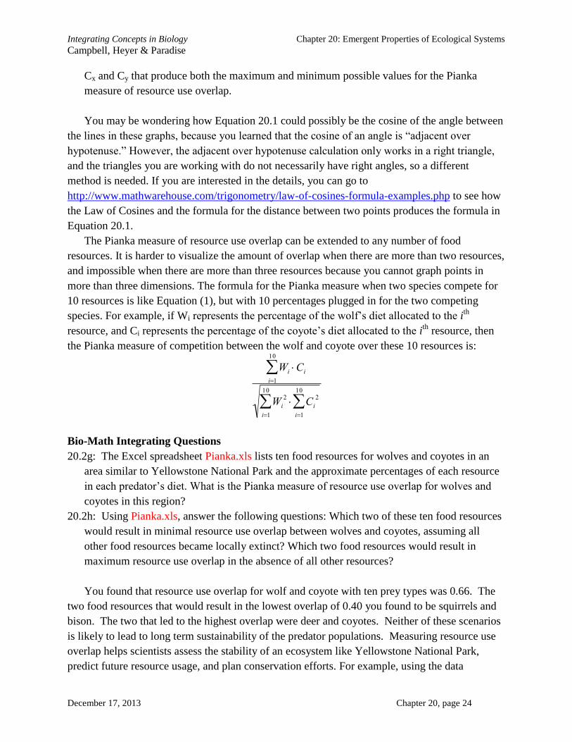
The Pianka measure of resource use overlap can be extended to any number of food
resources. It is harder to visualize the amount of overlap when there are more than two resources,
and impossible when there are more than three resources because you cannot graph points in
more than three dimensions. The formula for the Pianka measure when two species compete for
10 resources is like Equation (1), but with 10 percentages plugged in for the two competing
species. For example, if Wi represents the percentage of the wolf’s diet allocated to the ith
resource, and Ci represents the percentage of the coyote’s diet allocated to the ith
resource, then
the Pianka measure of competition between the wolf and coyote over these 10 resources is:
Wi Cii1
10
Wi
2
i1
10
Ci2
i1
10
Bio-Math Integrating Questions
20.2g: The Excel spreadsheet Pianka.xls lists ten food resources for wolves and coyotes in an
area similar to Yellowstone National Park and the approximate percentages of each resource
in each predator’s diet. What is the Pianka measure of resource use overlap for wolves and
coyotes in this region?
20.2h: Using Pianka.xls, answer the following questions: Which two of these ten food resources
would result in minimal resource use overlap between wolves and coyotes, assuming all
other food resources became locally extinct? Which two food resources would result in
maximum resource use overlap in the absence of all other resources?
You found that resource use overlap for wolf and coyote with ten prey types was 0.66. The
two food resources that would result in the lowest overlap of 0.40 you found to be squirrels and
bison. The two that led to the highest overlap were deer and coyotes. Neither of these scenarios
is likely to lead to long term sustainability of the predator populations. Measuring resource use
overlap helps scientists assess the stability of an ecosystem like Yellowstone National Park,
predict future resource usage, and plan conservation efforts. For example, using the data

Integrating Concepts in Biology Chapter 20: Emergent Properties of Ecological Systems
Campbell, Heyer & Paradise
December 17, 2013 Chapter 20, page 25
provided in Pianka.xls, ecologists could predict ways in which wolf and coyote behaviors might
evolve to reduce the degree of resource use overlap in Yellowstone National Park. Similarly,
conservation biologists could assess the resources and predict the possibility of extinction of
wolf competitors or the success of wolves when wolves were reintroduced to the Park.
---------------------------------------------------------------------------------------------------------------------
Species that have high resource use overlap coexist by altering their resource use when the
competing species is present. Coyotes may include a higher proportion of elk in their diet when
wolves are absent, but then switch to consuming more squirrels, rabbits and mice when wolves
are present. Resource use overlap can be relatively high in two coexisting species, but cannot be
100%. As overlap increases, species involved in competition may switch to unused, less
desirable resources, especially if they are abundant in the environment. This switching behavior
is a mechanism for species coexistence.
The outcome of competition depends on the species involved, but may also depend on
variation in abiotic factors in the environment. Ecological systems change across space, where
conditions related to an abiotic factor change as location changes. For example, average
temperatures become cooler as one moves from the equator toward the poles, or the moisture in
soil may decrease as you move upslope from a body of water towards higher ground. Another
type of change is across time, where the condition changes as time passes. A common example
is the variation in the amount of rain as seasons change from dry to rainy season. Some changes
take place over time and space. Consider an estuary, the region where rivers meet oceans. The
salt content of estuaries may change not only across space, as you move from a river delta
toward the ocean, but also across time, tides push in salty water or yield to fresh water in the
river. Changes in environmental properties across time or space are called environmental
gradients, and biologists often study how organisms respond to these gradients. {Definition: A
gradient is a change in an abiotic variable across time or space.}
Some conditions are harsher than others – for most plants, drier soils with fewer nutrients are
more stressful than wet, fertile soils. Disturbances such as fires or strong storms may also affect
the ability of an organism to survive. {Connections: Evolutionary adaptations to disturbance
are explored in Section 10.3.} Some scientists have hypothesized that organisms adapted to
living in harsh conditions, either because of high levels of disturbance or low levels of essential
nutrients, are poor competitors in less harsh conditions. If this hypothesis is correct, species
adapted to conditions of high nutrients or high resources would be better competitors when living
in conditions with high nutrients or resources.
You will examine one study that investigates this hypothesis about adaptation to harsh
conditions, but before you do, you should review the three main ideas about emergent properties
and apply them to this hypothesis. One main idea about emergent properties is that biological
systems require resources, which results in competition or cooperation for resources. Another
main idea about emergent properties is that randomness and variation within an ecological
system allow coexistence of species. Different species that consume the same resource (e.g.,
Integrating Concepts in Biology Chapter 20: Emergent Properties of Ecological Systems
Campbell, Heyer & Paradise
December 17, 2013 Chapter 20, page 26
plants competing for sunlight) may be adapted to live in different environmental conditions. For
example, plants compete for access to sunlight, but some plants are adapted to direct sunlight
while others prefer indirect light, which minimizes resource use overlap. Tall oak and pine trees
are adapted to more direct light conditions while shade-loving mosses and ferns specialize in low
light photosynthesis and yet all four plants consume the same resource. {Connections:
Adaptations to varying light conditions is explored in Section 9.4.} These plants don’t coexist at
the exact same location, but they can live near each other within in a wider ecological system,
such as a forest. The third main idea about emergent properties is that biological systems exceed
the sum of their parts. These ecological systems do so by increasing biodiversity in the forest,
causing indirect interactions, and changing the abiotic conditions of the forest.
Ecologists Scott Wilson and Paul Keddy tested the hypothesis that there is a trade-off
between competitive ability and adaptations to harsh conditions. They studied the distributions of
seven plant species along the shores of Axe Lake in Ontario, Canada where there exists an
environmental gradient. This environmental gradient included both changes in disturbance, in
the force of waves hitting the shore, and the amount of organic matter and nutrients in the soil.
The scientists quantified the organic matter content in many plots as a measure of the gradient
because they had found in previous research that organic matter negatively correlated with wave
action intensity – shores exposed to high wave action have lower levels of nutrients. Their study
sites ranged from exposed beaches with high wave action and low nutrient concentrations to
sheltered shores in small inlets with nutrient-
rich soils.
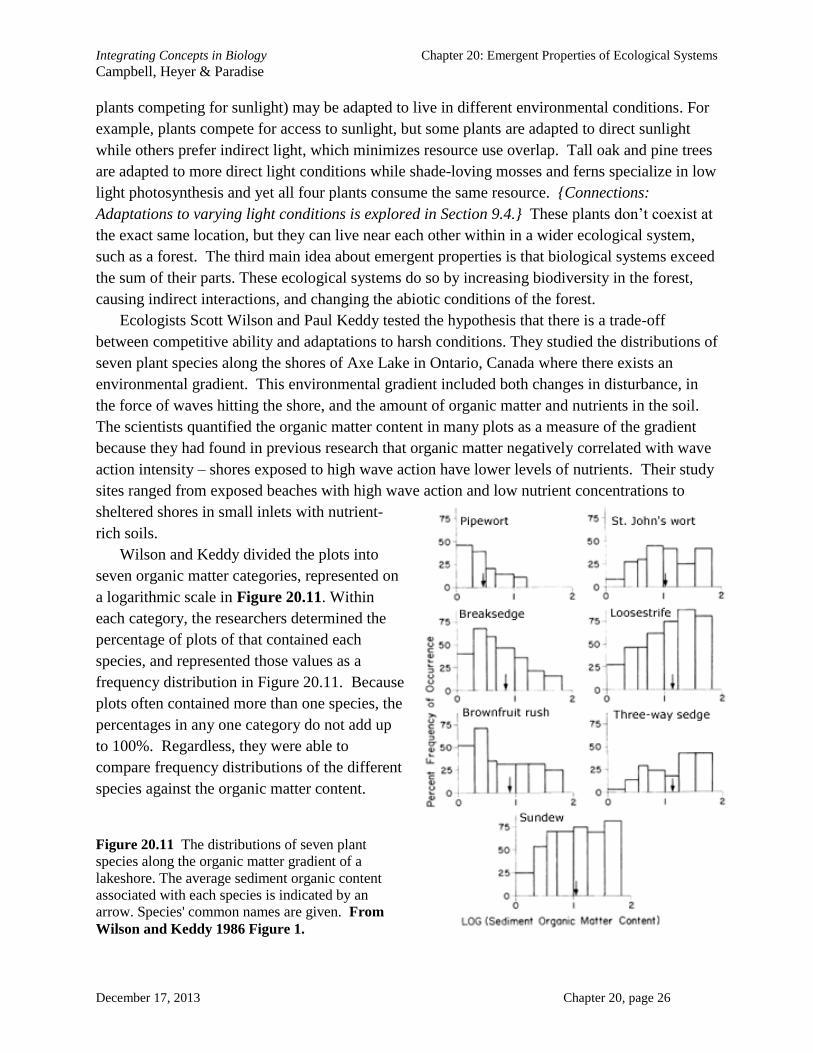
Wilson and Keddy divided the plots into
seven organic matter categories, represented on
a logarithmic scale in Figure 20.11. Within
each category, the researchers determined the
percentage of plots of that contained each
species, and represented those values as a
frequency distribution in Figure 20.11. Because
plots often contained more than one species, the
percentages in any one category do not add up
to 100%. Regardless, they were able to
compare frequency distributions of the different
species against the organic matter content.
Figure 20.11 The distributions of seven plant
species along the organic matter gradient of a
lakeshore. The average sediment organic content
associated with each species is indicated by an
arrow. Species' common names are given. From
Wilson and Keddy 1986 Figure 1.

Integrating Concepts in Biology Chapter 20: Emergent Properties of Ecological Systems
Campbell, Heyer & Paradise
December 17, 2013 Chapter 20, page 27
Integrating Questions
26. Consider the following factors and situations and describe how the factor changes across
space: water depth from the shore of a lake to its center, temperature from a grassy area to
the edge of a forest to the forest interior, salt concentration from the mouth of a river to an
estuary to the open ocean, moisture content of soil from the edge of a river to the top of a hill.
27. Compare and contrast the frequency distributions of the seven plants. A frequency
distribution in this case would be the percentage of plots in which each of the seven plants
was found at each concentration of organic matter.
28. Are there any plants that appear similar in resource and habitat use, and if so, which ones?
29. Organic matter content is an indication of harshness and disturbance. According to the trade-
off hypothesis stated previously, which species do you predict will be poor competitors?
Superior competitors?
Once Wilson and Keddy plotted their data, they observed clear differences in the
distributions of the plants. Some plants had higher frequencies of occurrence at lower organic
matter levels while others had higher frequencies at the high end of the organic matter scale.
Wilson and Keddy designed an experiment to determine the competitive abilities of each plant
species compared to the other six species. The scientists placed two plants, one from each of two
different species or two from the same species, in a small bucket filled with sand and organic
shoreline sediment, simulating a sheltered shore with high organic matter. They had ten buckets
of each pair-wise combination of species for a total of 490 buckets.
The scientists measured relative growth, growth in the presence of another species compared
to growth in the presence of another member of the same species, as an indication of competitive
ability. They quantified their comparative growth using a value they called relative increase per
plant (RIP). Growth was determined by measuring biomass at the time of planting and again at
the time of harvest about three months later. Since the biomass measurement kills the plants, the
initial measurements were made on a random sample of plants of the same size as those planted,
sacrificed for that purpose. To calculate RIP at the end of the experiment, they determined the
average final biomass of plants of species i grown in the presence of plants of species j minus the
average initial biomass of plants of species i. They then divided that quantity by the average
final biomass of a plant of species i grown in the presence of a plant of species i minus initial
biomass of species i.
(final biomass of i with j) – (initial biomass of i)
RIPij = --------------------------------------------------------------
(final biomass of i with i) – (initial biomass of i)
Table 20.1 lists their results. {Definitions: Biomass is the total mass of a living organism after
removal of water, often expressed or referred to as dry mass.}
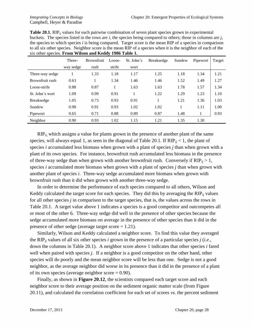
Integrating Concepts in Biology Chapter 20: Emergent Properties of Ecological Systems
Campbell, Heyer & Paradise
December 17, 2013 Chapter 20, page 28
Table 20.1. RIPij values for each pairwise combination of seven plant species grown in experimental
buckets. The species listed in the rows are i, the species being compared to others; those in columns are j,
the species to which species i is being compared. Target score is the mean RIP of a species in comparison
to all six other species. Neighbor score is the mean RIP of a species when it is the neighbor of each of the
six other species. From Wilson and Keddy 1986 Table 1.
Three-
way sedge
Brownfruit
rush
Loose-
strife
St. John’s
wort
Breaksedge Sundew Pipewort Target
Three-way sedge 1 1.33 1.18 1.17 1.25 1.18 1.34 1.21
Brownfruit rush 0.63 1 1.34 1.46 1.46 1.52 1.49 1.27
Loose-strife 0.88 0.87 1 1.63 1.63 1.78 1.57 1.34
St. John’s wort 1.09 0.99 0.91 1 1.22 1.29 1.23 1.10
Breaksedge 1.05 0.73 0.93 0.91 1 1.21 1.36 1.03
Sundew 0.98 0.91 0.93 1.02 1.02 1 1.11 1.00
Pipewort 0.65 0.71 0.88 0.89 0.87 1.48 1 0.93
Neighbor 0.90 0.93 1.02 1.15 1.21 1.35 1.30
RIPii, which assigns a value for plants grown in the presence of another plant of the same
species, will always equal 1, as seen in the diagonal of Table 20.1. If RIPij < 1, the plant of
species i accumulated less biomass when grown with a plant of species j than when grown with a
plant of its own species. For instance, brownfruit rush accumulated less biomass in the presence
of three-way sedge than when grown with another brownfruit rush. Conversely if RIPij > 1,
species i accumulated more biomass when grown with a plant of species j than when grown with
another plant of species i. Three-way sedge accumulated more biomass when grown with
brownfruit rush than it did when grown with another three-way sedge.
In order to determine the performance of each species compared to all others, Wilson and
Keddy calculated the target score for each species. They did this by averaging the RIPij values
for all other species j in comparison to the target species, that is, the values across the rows in
Table 20.1. A target value above 1 indicates a species is a good competitor and outcompetes all
or most of the other 6. Three-way sedge did well in the presence of other species because the
sedge accumulated more biomass on average in the presence of other species than it did in the
presence of other sedge (average target score = 1.21).
Similarly, Wilson and Keddy calculated a neighbor score. To find this value they averaged
the RIPij values of all six other species i grown in the presence of a particular species j (i.e.,
down the columns in Table 20.1). A neighbor score above 1 indicates that other species i fared
well when paired with species j. If a neighbor is a good competitor on the other hand, other
species will do poorly and the mean neighbor score will be less than one. Sedge is not a good
neighbor, as the average neighbor did worse in its presence than it did in the presence of a plant
of its own species (average neighbor score = 0.90).
Finally, as shown in Figure 20.12, the scientists compared each target score and each
neighbor score to their average position on the sediment organic matter scale (from Figure
20.11), and calculated the correlation coefficient for each set of scores vs. the percent sediment

Integrating Concepts in Biology Chapter 20: Emergent Properties of Ecological Systems
Campbell, Heyer & Paradise
December 17, 2013 Chapter 20, page 29
organic matter content. Recall from BME x.x that correlation coefficients range from -1 to +1,
and measure the strength and direction of a linear relationship between two variables.
a value of -1 indicates a strong negative linear relationship; one variable increases as the
other decreases;
a value of 0 indicates no relationship;
a value of +1 indicates a strong positive linear relationship; one variable increases as the
other increases.
Figure 20.12 a. The relationship
between target scores and percent
sediment organic matter content for the
seven species at Axe Lake, Ontario. b.
The relationship between neighbor
scores and percent sediment organic
matter content for the seven species.
Correlation coefficients are given for
each panel. PW = pipewort, BS =
breaksedge, BFR = brownfruit rush,
LS = loosestrife, TWS = three-way
sedge, SJW = St John’s wort, and SD
= sundew. From Wilson and Keddy
1986 Figure 2.
Integrating Questions
30. Which species is a better
competitor, brownfruit rush or
three-way sedge (see Table 20.1
and the description in the text)?
31. The sundew was excluded from
the correlation analysis in Figure
20.12. Examination of both graphs
may provide a clue as to why the
analysis omitted sundew. In
addition, sundew is insectivorous.
What does insectivorous mean, and what are the resource implications for competition
between sundew and the other plants in this ecological system? Search the textbook website
or the Encyclopedia of Earth site (http://www.eoearth.org) for information on insectivorous
plants. Specifically, look for information on sundews.
32. How do target and neighbor scores in the plant community change as percent sediment
organic matter increases? On each graph in Figure 20.12, indicate the dependent and the
independent variable. Which dependent variable of competitive advantage has a negative

Integrating Concepts in Biology Chapter 20: Emergent Properties of Ecological Systems
Campbell, Heyer & Paradise
December 17, 2013 Chapter 20, page 30
relationship with the independent variable, and which one has a positive relationship? Do the
relationships fit the pattern predicted by the scientists?
You began this case study by asking whether there were emergent properties associated with
competition for limited resources. You have discovered that plants with high competitive ability
tend to occupy sheltered, nutrient-rich shores, while species with low competitive ability occupy
disturbed shorelines with low nutrient content soils. This make sense since those who compete
best get the best growing conditions, while those that compete poorly must adapt to worse soil
conditions or face extinction.
From the analysis of Wilson and Keddy, you saw that the sundew is not a very good
competitor in high organic matter soils, having the second lowest target score, and only does
better in head-to-head competition with pipewort. And sundew is also a very good neighbor,
with the other six species outcompeting sundew in the experiment. Because of sundew’s ability
to acquire extra nutrients from insects, the researchers did not include this species in the
correlation analysis. Under the conditions of the experiment, sundew did not perform well, but
along the shores of the lake, sundew actually does compete well, and tends to be found in more
favorable conditions. The nutrients from insects give it a competitive edge.
Adaptations to particular environmental conditions such as disturbance and soil nutrient
concentrations determine where species can live, which directly or indirectly determine the
outcome of competition. The property that emerges from all this is a diverse community of plant
species that coexist at a location (such as the shore of a lake) and yet use a variety of
microhabitats. {Connections: Microhabitats are explored in Section 8.3.} Plants provide
resources to many microbial and animal species that benefit from these different plants. The
beneficiaries of the plants have, in turn, different competitive abilities and adaptations that they
need to feed on particular plants. All these different interactions lead to increased complexity and
the potential for indirect interactions in ecological systems – a good example of an emergent
property at the ecological system scale.
Although the seven plants exhibit a significant amount of overlap in distributions at Axe
Lake, Ontario, the sundew has adapted very well to living in conditions in which the other
species cannot exist. You would not expect plants to evolve to be less competitive and adapt to
low-nutrient growth conditions. But growth in nutrient poor conditions is better than going
extinct after competing and losing out to a more competitive species. You have uncovered an
evolutionary mechanism involving competing species: a species may adapt to exploit a resource
more efficiently, and become a superior competitor (target score > 1). Alternatively, a species
with low target scores may adapt to live in an environment from which superior competitors are
excluded, or it may adapt to exploit a different resource altogether. Adapting to an alternative
means to acquire a limited resource is an explanation for sundew, the carnivorous plant. In the
next study you will examine competition for a different type of resource, but one that also
involves the introduction of new species to an area and habitat alterations by humans.
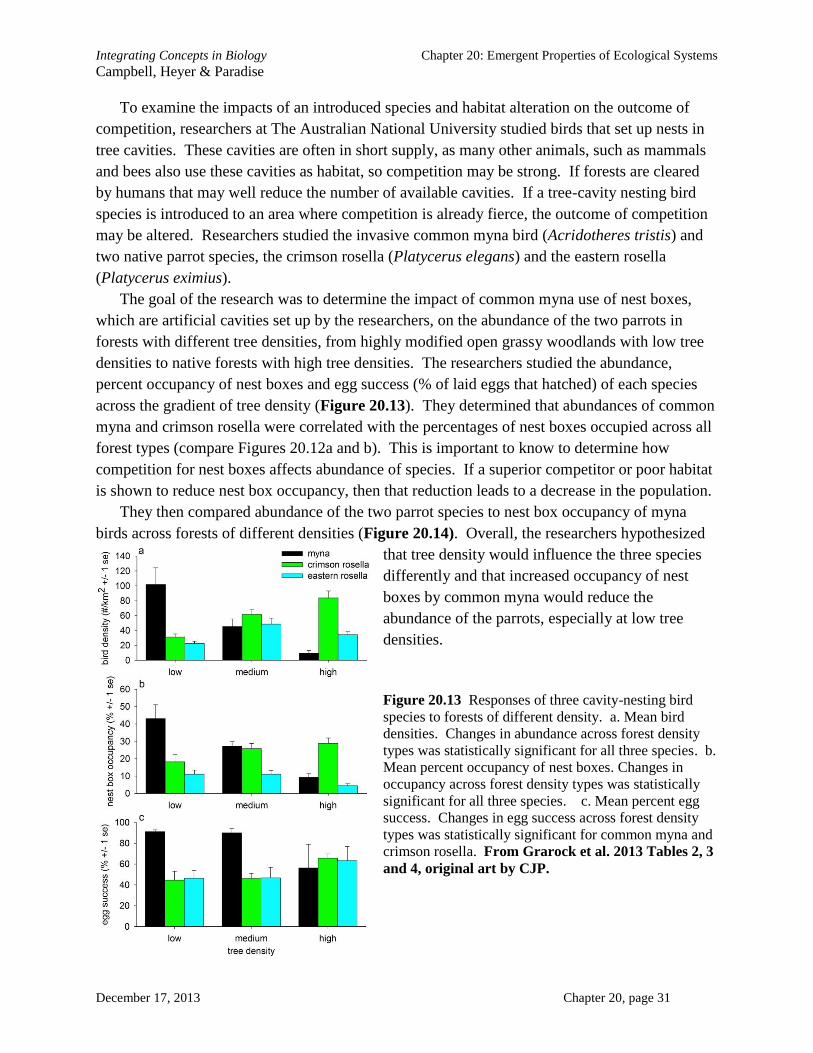
Integrating Concepts in Biology Chapter 20: Emergent Properties of Ecological Systems
Campbell, Heyer & Paradise
December 17, 2013 Chapter 20, page 31
To examine the impacts of an introduced species and habitat alteration on the outcome of
competition, researchers at The Australian National University studied birds that set up nests in
tree cavities. These cavities are often in short supply, as many other animals, such as mammals
and bees also use these cavities as habitat, so competition may be strong. If forests are cleared
by humans that may well reduce the number of available cavities. If a tree-cavity nesting bird
species is introduced to an area where competition is already fierce, the outcome of competition
may be altered. Researchers studied the invasive common myna bird (Acridotheres tristis) and
two native parrot species, the crimson rosella (Platycerus elegans) and the eastern rosella
(Platycerus eximius).
The goal of the research was to determine the impact of common myna use of nest boxes,
which are artificial cavities set up by the researchers, on the abundance of the two parrots in
forests with different tree densities, from highly modified open grassy woodlands with low tree
densities to native forests with high tree densities. The researchers studied the abundance,
percent occupancy of nest boxes and egg success (% of laid eggs that hatched) of each species
across the gradient of tree density (Figure 20.13). They determined that abundances of common
myna and crimson rosella were correlated with the percentages of nest boxes occupied across all
forest types (compare Figures 20.12a and b). This is important to know to determine how
competition for nest boxes affects abundance of species. If a superior competitor or poor habitat
is shown to reduce nest box occupancy, then that reduction leads to a decrease in the population.
They then compared abundance of the two parrot species to nest box occupancy of myna
birds across forests of different densities (Figure 20.14). Overall, the researchers hypothesized
that tree density would influence the three species
differently and that increased occupancy of nest
boxes by common myna would reduce the
abundance of the parrots, especially at low tree
densities.
Figure 20.13 Responses of three cavity-nesting bird
species to forests of different density. a. Mean bird
densities. Changes in abundance across forest density
types was statistically significant for all three species. b.
Mean percent occupancy of nest boxes. Changes in
occupancy across forest density types was statistically
significant for all three species. c. Mean percent egg
success. Changes in egg success across forest density
types was statistically significant for common myna and
crimson rosella. From Grarock et al. 2013 Tables 2, 3
and 4, original art by CJP.
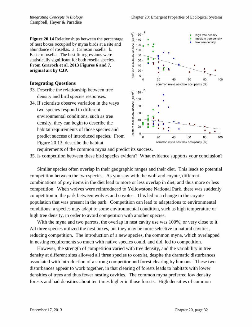
Integrating Concepts in Biology Chapter 20: Emergent Properties of Ecological Systems
Campbell, Heyer & Paradise
December 17, 2013 Chapter 20, page 32
Figure 20.14 Relationships between the percentage
of nest boxes occupied by myna birds at a site and
abundance of rosellas. a. Crimson rosella. b.
Eastern rosella. The best fit regressions were
statistically significant for both rosella species.
From Grarock et al. 2013 Figures 6 and 7,
original art by CJP.
Integrating Questions
33. Describe the relationship between tree
density and bird species responses.
34. If scientists observe variation in the ways
two species respond to different
environmental conditions, such as tree
density, they can begin to describe the
habitat requirements of those species and
predict success of introduced species. From
Figure 20.13, describe the habitat
requirements of the common myna and predict its success.
35. Is competition between these bird species evident? What evidence supports your conclusion?
Similar species often overlap in their geographic ranges and their diet. This leads to potential
competition between the two species. As you saw with the wolf and coyote, different
combinations of prey items in the diet lead to more or less overlap in diet, and thus more or less
competition. When wolves were reintroduced to Yellowstone National Park, there was suddenly
competition in the park between wolves and coyotes. This led to a change in the coyote
population that was present in the park. Competition can lead to adaptations to environmental
conditions: a species may adapt to some environmental condition, such as high temperature or
high tree density, in order to avoid competition with another species.
With the myna and two parrots, the overlap in nest cavity use was 100%, or very close to it.
All three species utilized the nest boxes, but they may be more selective in natural cavities,
reducing competition. The introduction of a new species, the common myna, which overlapped
in nesting requirements so much with native species could, and did, led to competition.
However, the strength of competition varied with tree density, and the variability in tree
density at different sites allowed all three species to coexist, despite the dramatic disturbances
associated with introduction of a strong competitor and forest clearing by humans. These two
disturbances appear to work together, in that clearing of forests leads to habitats with lower
densities of trees and thus fewer nesting cavities. The common myna preferred low density
forests and had densities about ten times higher in those forests. High densities of common
Integrating Concepts in Biology Chapter 20: Emergent Properties of Ecological Systems
Campbell, Heyer & Paradise
December 17, 2013 Chapter 20, page 33
myna led to high percent occupancy of nest boxes and greater success of eggs. Something in the
low density forests allowed myna birds to be more successful.
Low tree density forests might naturally have low densities of rosellas. However, just as you
concluded from your examination of the data, the researchers were able to show that in those
habitats high tree densities of myna birds led to high occupancy of nest boxes and that reduced
the abundance of crimson and eastern rosellas. When mynas were less abundant, as in the
medium and high tree density forests, abundance, nest box occupancy and egg success all went
up, to different degrees, in the two rosella species.
You have learned that changes in an environmental condition, in this case forest tree density,
strongly influenced the outcome of competition for a limiting resource, in this case, nest boxes.
The outcome of competition was determined partly by the differential use of habitat by the birds
determined by their different genetically encoded responses to variable forest types. {Definition:
a limiting resource is a resource, such as food, light, nutrients, or space, which is in short supply
and restricts the growth of an organism or population.}
You began this section by considering competition for resources and the variability in
environmental conditions. The results of the studies demonstrated all three of the main ideas of
emergent properties. Adaptations to different habitats led to the evolution of diverse species that
utilize similar resources within an ecosystem, in such a way that they can coexist in a broad
geographical region. Species diversity is an emergent property of ecological systems – the
ecosystem, with its individual species all living in the same region, is more than the sum of its
parts. Competition for resources led species to evolve adaptations to exist in different
microhabitats – the three bird species have adapted to slightly different conditions, which often
helps avoid direct competition and possible extinction. The three bird species were able to
coexist together, even though densities of rosellas were reduced in the presence of high myna
density, possibly because the birds competed less for other resources, such as food.
20.3 How efficient are ecological systems at transferring energy from the sun and carbon
dioxide from the air to predators?
Context: Energy from the sun and carbon dioxide from the atmosphere enter and move
through ecological systems.
Major Themes: Biological systems exceed the sum of their parts, randomness within a
biological system provides flexibility of response, and biological systems require resources,
which results in competition or cooperation.
Bottom Line: Energy and nutrients are transferred between trophic levels via feeding
relationships.
In the first two sections of this chapter, you focused on emergent properties that arise in
ecological systems as a result of predator-prey or competitive interactions. Each of these types
of interactions affects the flow of energy and nutrients within an ecological system. Energy
flows are emergent properties and you will examine them in more detail here. Ecological
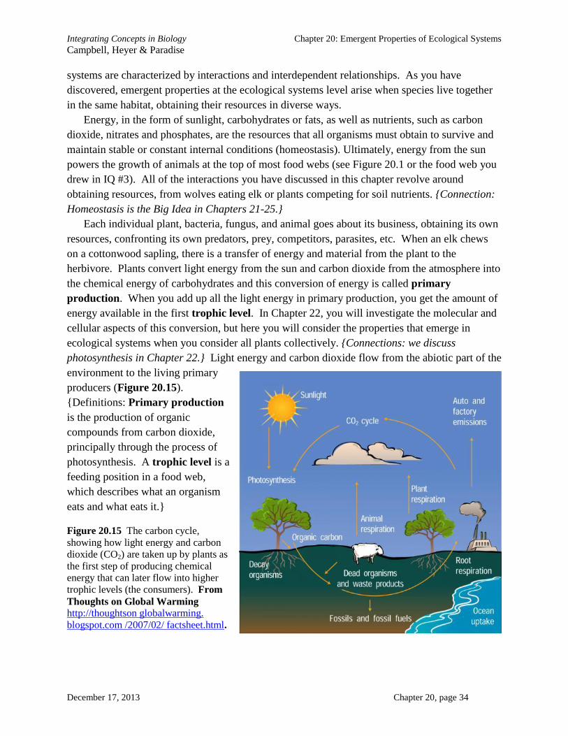
Integrating Concepts in Biology Chapter 20: Emergent Properties of Ecological Systems
Campbell, Heyer & Paradise
December 17, 2013 Chapter 20, page 34
systems are characterized by interactions and interdependent relationships. As you have
discovered, emergent properties at the ecological systems level arise when species live together
in the same habitat, obtaining their resources in diverse ways.
Energy, in the form of sunlight, carbohydrates or fats, as well as nutrients, such as carbon
dioxide, nitrates and phosphates, are the resources that all organisms must obtain to survive and
maintain stable or constant internal conditions (homeostasis). Ultimately, energy from the sun
powers the growth of animals at the top of most food webs (see Figure 20.1 or the food web you
drew in IQ #3). All of the interactions you have discussed in this chapter revolve around
obtaining resources, from wolves eating elk or plants competing for soil nutrients. {Connection:
Homeostasis is the Big Idea in Chapters 21-25.}
Each individual plant, bacteria, fungus, and animal goes about its business, obtaining its own
resources, confronting its own predators, prey, competitors, parasites, etc. When an elk chews
on a cottonwood sapling, there is a transfer of energy and material from the plant to the
herbivore. Plants convert light energy from the sun and carbon dioxide from the atmosphere into
the chemical energy of carbohydrates and this conversion of energy is called primary
production. When you add up all the light energy in primary production, you get the amount of
energy available in the first trophic level. In Chapter 22, you will investigate the molecular and
cellular aspects of this conversion, but here you will consider the properties that emerge in
ecological systems when you consider all plants collectively. {Connections: we discuss
photosynthesis in Chapter 22.} Light energy and carbon dioxide flow from the abiotic part of the
environment to the living primary
producers (Figure 20.15).
{Definitions: Primary production
is the production of organic
compounds from carbon dioxide,
principally through the process of
photosynthesis. A trophic level is a
feeding position in a food web,
which describes what an organism
eats and what eats it.}
Figure 20.15 The carbon cycle,
showing how light energy and carbon
dioxide (CO2) are taken up by plants as
the first step of producing chemical
energy that can later flow into higher
trophic levels (the consumers). From
Thoughts on Global Warming http://thoughtson globalwarming.
blogspot.com /2007/02/ factsheet.html.
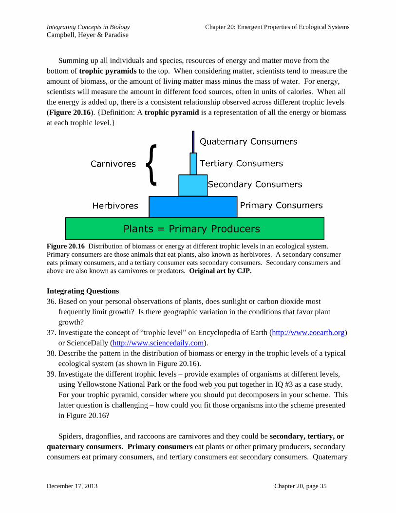
Integrating Concepts in Biology Chapter 20: Emergent Properties of Ecological Systems
Campbell, Heyer & Paradise
December 17, 2013 Chapter 20, page 35
Summing up all individuals and species, resources of energy and matter move from the
bottom of trophic pyramids to the top. When considering matter, scientists tend to measure the
amount of biomass, or the amount of living matter mass minus the mass of water. For energy,
scientists will measure the amount in different food sources, often in units of calories. When all
the energy is added up, there is a consistent relationship observed across different trophic levels
(Figure 20.16). {Definition: A trophic pyramid is a representation of all the energy or biomass
at each trophic level.}
Figure 20.16 Distribution of biomass or energy at different trophic levels in an ecological system.
Primary consumers are those animals that eat plants, also known as herbivores. A secondary consumer
eats primary consumers, and a tertiary consumer eats secondary consumers. Secondary consumers and
above are also known as carnivores or predators. Original art by CJP.
Integrating Questions
36. Based on your personal observations of plants, does sunlight or carbon dioxide most
frequently limit growth? Is there geographic variation in the conditions that favor plant
growth?
37. Investigate the concept of “trophic level” on Encyclopedia of Earth (http://www.eoearth.org)
or ScienceDaily (http://www.sciencedaily.com).
38. Describe the pattern in the distribution of biomass or energy in the trophic levels of a typical
ecological system (as shown in Figure 20.16).
39. Investigate the different trophic levels – provide examples of organisms at different levels,
using Yellowstone National Park or the food web you put together in IQ #3 as a case study.
For your trophic pyramid, consider where you should put decomposers in your scheme. This
latter question is challenging – how could you fit those organisms into the scheme presented
in Figure 20.16?
Spiders, dragonflies, and raccoons are carnivores and they could be secondary, tertiary, or
quaternary consumers. Primary consumers eat plants or other primary producers, secondary
consumers eat primary consumers, and tertiary consumers eat secondary consumers. Quaternary

Integrating Concepts in Biology Chapter 20: Emergent Properties of Ecological Systems
Campbell, Heyer & Paradise
December 17, 2013 Chapter 20, page 36
consumers are usually the top predators that consume tertiary (and often secondary and primary)
consumers. Going back to our original question, how does light energy from the sun get
incorporated into a dragonfly’s body? Let’s consider a classic study in ecology by John Teal
who studied salt marshes of Georgia along the southeastern coast of the United States. A salt
marsh is part of an estuary, the waters between oceans and rivers. You will consider some
research on these ecological systems performed by Teal and his colleagues. {Definitions:
Primary consumers are organisms that get their energy from primary producers (plants), also
known as herbivores. Secondary, tertiary, and quaternary consumers are organisms that get
their energy from other consumers. These are often called carnivores. Secondary consumers eat
primary consumers, tertiary consumers eat secondary consumers, etc.}
Salt marshes are bounded on one side by sea islands and on the other, by the mainland. The
salt concentrations of the marsh fluctuate with the amount of rainfall and the height of the tides.
You know from examination of killifish that some species have adapted to these harsh and
dynamic conditions. Salt-tolerant smooth cordgrass makes up most of grass in the salt marshes.
However, there is a gradient of habitat types (Figure 20.17).
Figure 20.17 Range of habitats typically observed in a salt marsh and surrounding terrestrial zone.
Notice how the vegetation type changes as distance from the tidal creek increases. The tidal creek rises
and falls with the tides, and can reach as far as the high marsh, but only rarely, leaving salty water behind
when it recedes. From Sherpa Guides, The Natural History of Georgia's Barrier Islands
http://www.sherpaguides.com/georgia/barrier_islands/natural_history/index.html.
Cordgrass dominates in tidal creek, levee, and low marsh zones and thus is the dominant primary
producer. Algae species floating in the water are also important primary producers, whereas
other plants dominate the drier zones.
Teal listed the obvious species occurring in each zone, although he focused his research on
the low saltmarsh. From knowledge of these animals, plants, and microbes, he constructed the
food web shown in Figure 20.18.

Integrating Concepts in Biology Chapter 20: Emergent Properties of Ecological Systems
Campbell, Heyer & Paradise
December 17, 2013 Chapter 20, page 37
Figure 20.18 Recreation of Teal’s saltmarsh foodweb. The lower group of herbivores, as classified by
Teal, are feeding on both living algae and dead cordgrass that sinks to the bottom of the marsh. Bacteria
are feeding on decomposing organic matter – the cordgrass and animals that die are decomposed by
bacteria. From Teal 1962 Figure 2, original art by CJP.
Teal and his colleagues estimated 34,580 kilocalories / m2 / year of primary production in the salt
marsh, which is how much energy was converted from carbon dioxide and sunlight into
carbohydrates. The actual amount of plant biomass growth, however, was estimated to be only
6,580 kilocalories / m2 / year. Dividing the biomass energy (6,580) by total chemical energy
(34,580) tells us that only 19% of the total chemical energy is retained in the plant biomass. Teal
measured algal production and biomass, too. The efficiency of conversion of primary production
to biomass was higher for algae, although the total amount of production was lower (1,620
(biomass growth) ÷ 1,800 (total primary production) kilocalories / m2 / year = 90%). The total
biomass growth for all primary producers (6,580 + 1,620 = 8,200 kilocalories / m2 / year) is what
is available to primary consumers (herbivores).
Let’s focus only on the upper pathway in Figure 20.18, especially the small jumping insects
called planthoppers and katydids, a type of grasshopper. Teal and his colleagues estimated the
annual amount of energy in the insects’ consumption, production, respiration, assimilation, and
waste (Figure 20.19).

Integrating Concepts in Biology Chapter 20: Emergent Properties of Ecological Systems
Campbell, Heyer & Paradise
December 17, 2013 Chapter 20, page 38
Figure 20.19 Energy relationships in saltmarsh planthoppers and katydids. Estimates are from Teal
(1962). He estimated 85% assimilation efficiency for planthoppers because they feed on liquid sugar
solutions from plants, which are easy to digest, not cellulose, which is a plant structural chemical that is
not easy to digest. The assimilation efficiency for grasshoppers, which consume mostly cellulose, was
estimated to be 30%. From Teal 1962, data in text, original art by CJP.
After eating, the food is either assimilated into the body via the digestive system, or eliminated
as feces. Of the assimilated food, some goes to growth (production) and some goes to respiration
(ATP production and CO2 waste). Respiration is sort of the opposite of photosynthesis – carbon
dioxide is a waste product of cellular respiration, which puts carbon dioxide back into the
environment for plants to absorb again during photosynthesis. {Connections: Cellular
respiration is discussed in Chapter 21.} Thus, carbon cycles in the environment (i.e., CO2 →
biomass → CO2). Nutrient cycling is an emergent property of ecological systems and occurs as
organisms grow, consume, and respire (Figure 20.20).
323.5
275.0
70.0
205.0
48.5
99.4
29.410.8
18.6
70.0
0.0
50.0
100.0
150.0
200.0
250.0
300.0
350.0
Consumption Assimilation Production Respiration Feces
Ene
rgy (
kca
l /
m2
/ y
ear
Planthoppers
Katydids

Integrating Concepts in Biology Chapter 20: Emergent Properties of Ecological Systems
Campbell, Heyer & Paradise
December 17, 2013 Chapter 20, page 39
Figure 20.20 One pathway of energy and carbon in the Georgia saltmarsh. Carbon cycles (atmosphere
plants herbivores carnivores atmosphere), and each component sends carbon dioxide back to the
atmosphere. Decomposers also respire or provide biomass to predators. The pathway of carbon is
combined with energy flow (sunlight plants herbivores carnivores, with respiration energy used
for metabolism and lost as heat). The size of the boxes for cordgrass, insects herbivores, and predators is
proportional to the energy content in each trophic level. From Teal 1962 Figure 4 and data in text,
original art by CJP.
The amount of production of the two herbivorous insect species is available for consumption
by spiders, wrens, and dragonflies (Figure 20.18). Spiders are the most abundant predator of
these two insects, but Teal lumped all predators together for his analysis. Teal estimated that
together predators consumed 28 out of 80.8 kilocalories / m2 / year available to them in the form
of planthopper and katydid biomass. The rest of the insect herbivore biomass (52.8 kilocalories /
m2 / year) ended up as food for bacteria or was washed out of the saltmarsh when the insects
died. The predators converted those 28 kilocalories into only 5 kilocalories / m2 / year of
biomass production.
Integrating Questions
40. Examine Figure 20.17 and develop hypotheses to explain what factors determine the type of
habitat that appears along this gradient. Consider what you know about saltmarshes, or
conduct an internet search if you need more information

Integrating Concepts in Biology Chapter 20: Emergent Properties of Ecological Systems
Campbell, Heyer & Paradise
December 17, 2013 Chapter 20, page 40
(http://www.sherpaguides.com/georgia/barrier_islands/natural_history/index.html has a good
description of the saltmarsh ecosystem). Can you design an experiment to test your
hypotheses?
41. Teal estimated that only 6.1% of the energy in sunlight was absorbed by the primary
producers in the Georgia saltmarsh. Why are plants only able to absorb this small fraction of
the sunlight? For this question, you may have to consult the WileyPlus tutorial on
photosynthesis and consider the properties of light and the wavelengths that plants are able to
use to convert carbon dioxide to carbohydrates.
42. What happens to the 81% of chemical energy produced by cordgrass that is not turned into
biomass? Consider other ways that plants use energy.
43. Which species has a higher assimilation efficiency (assimilation energy ÷ energy in
consumption), planthoppers or katydids? Which species has a higher production efficiency
(production energy ÷ assimilation energy), planthoppers or katydids? What do you conclude
about these efficiencies? Where does the energy go that is not assimilated? Where does the
energy go that is not used for production?
44. Calculate the percentage of energy in the cordgrass that is incorporated into predator
biomass. What value did you obtain? Why is this number so low?
As you have no doubt discovered, ecological systems are not very efficient. Most of the
energy captured by primary producers is lost through respiration. No organisms can use all of
the energy they consume to grow bigger – each must use energy to maintain basic metabolic
functions, to move or to reproduce. Much of the chemical energy used for metabolism or
reproduction is lost to as heat, which is waste energy. Because of this waste, the amount of
energy or biomass in predator trophic levels will always be smaller than the amount of energy or
biomass of the producer trophic level. After using the energy in carbohydrates, the carbon is
released as carbon dioxide into the atmosphere, where it is available for plants to consume again
in a continuous cycle. The heat energy is no longer available for organisms to use as a source of
energy for creating biomass and so this energy is biologically out of circulation. You have seen
how energy flows and nutrients cycle through ecological systems and their movement are
emergent properties that arise from the species that interact within an ecological system.
Conclusions
Emergent properties at any level of biological hierarchy cannot be studied in isolation. You
have learned that the other big ideas of biology, such as evolution, cells as functional units,
information, and homeostasis all contribute to emergent properties. For instance, any interaction
between two species may result in selective pressures and possible extinction, which is an
emergent property. Information is used by individuals to assess the environment while foraging
or maintaining homeostasis. What have you learned about emergent properties in ecological
systems? First, indirect effects arise from biotic interactions – the wolf-elk predator-prey
interaction led to effects on trees and several other animal species in Yellowstone National Park.

Integrating Concepts in Biology Chapter 20: Emergent Properties of Ecological Systems
Campbell, Heyer & Paradise
December 17, 2013 Chapter 20, page 41
Next, you learned that cooperation is an emergent property exhibited by packs of wolves as they
compete in an ecological system. You have also learned that species adapt to local environmental
conditions, which allows species to coexist even when they are competing for similar resources.
This leads to increased species diversity within an ecological system. Finally, you have learned
that nutrients cycle and energy flows in ecological systems, and those movements of matter and
energy arise from interactions between species, as herbivores eat plants and carnivores eat
herbivores.
End of Chapter Review Materials
Review Questions
1. What is a resource, and what are the consequences of a limiting resource?
2. Give an example of an indirect effect.
3. How does variation in ecological systems lead to “flexible responses”?
4. How do prey (individuals or populations) change as a result of exposure to a predator?
5. Explain how management of large mammalian herbivores by humans is unlike regulation of
those populations by their natural prey.
6. What is the competitive exclusion principle?
7. What hypothesis did scientists develop regarding competitive ability and adaptations to
abiotic conditions?
8. How do environmental conditions affect the outcome of competitive interactions?
9. What is a negative correlation between two variables?
10. What is primary production?
11. Why are transfers of energy between trophic levels less than 100% efficient?
12. What are trophic levels and trophic pyramids?
Apply What You Know
1. Predict the indirect effects of loss of another top predator from a marine ecosystem. What do
you think will happen to kelp forests in the ocean when sea otters are reduced in number,
considering that sea otters eat sea urchins, which eat kelp?
2. We learned that competitive interactions may be altered by environmental conditions. We
also learned that wolves and coyotes compete in Yellowstone National Park, and that wolves
appear to be outcompeting coyotes. Design an experiment to test the hypothesis that coyotes
are the superior competitors in some habitats.
3. Construct a trophic pyramid, like the one depicted in the Georgia saltmarsh, for the
Yellowstone ecosystem.
4. We learned how energy and carbon moved in tandem within ecological systems, from
primary producers to top predators. Predict how energy is also linked to other essential
biological elements, such as nitrogen and phosphorous.
Integrating Concepts in Biology Chapter 20: Emergent Properties of Ecological Systems
Campbell, Heyer & Paradise
December 17, 2013 Chapter 20, page 42
5. Speculate about an emergent property that arises when a squirrel collects and buries acorns
from oak trees.
6. How do the decisions made by individual predators or prey affect an entire population of the
same species?
7. Consider the evolution of cooperative behavior. If individual birds, for instance, attempt to
maximize the number of offspring they produce, relative to other individuals of the same
species, why would individuals choose to cooperate? There are only so many resources to go
around, and if one bird helps another, doesn’t it lose out on potential resource gains?
References
Wolves and Yellowstone National Park
Arjo WM, Pletscher DH, and Ream RR (2002) Dietary Overlap between Wolves and Coyotes in
Northwestern Montana. Journal of Mammalogy 83(3):754-766.
Beschta RL (2003) Cottonwoods, Elk, and Wolves in the Lamar Valley of Yellowstone National
Park. Ecological Applications 13(5):1295-1309.
Beschta RL (2005) Reduced Cottonwood Recruitment Following Extirpation of Wolves in
Yellowstone's Northern Range. Ecology 86(2):391-403.
Beschta RL and Ripple WJ (2012) Berry-producing shrub characteristics following wolf
reintroduction in Yellowstone National Park. Forest Ecology and Management 276:132–
138.
Creel S, Winnie J. Jr., Maxwell B, Hamlin K, and Creel M (2005) Elk Alter Habitat Selection as
an Antipredator Response to Wolves. Ecology 86(12):3387-3397.
Pianka ER (1973) The structure of lizard communities. Annual Review of Ecology and
Systematics 4:53-74.
Ripple WJ and Beschta RL (2004) Wolves and the Ecology of Fear: Can Predation Risk
Structure Ecosystems? BioScience 54(8):755-766.
Ripple WJ and Beschta RL (2007) Restoring Yellowstone’s aspen with wolves. Biological
Conservation 138:514 –519.
Robbins J (2004) Lessons from the wolf. Scientific American June 2004:76-81.
Smith DW, Stahler DR, and Guernsey DS (2006) Yellowstone Wolf Project: Annual Report,
2005. National Park Service, Yellowstone Center for Resources, Yellowstone National
Park, Wyoming, YCR-2006-04.
White PJ, and Garrott RA (2005) Northern Yellowstone Elk after Wolf Restoration. Wildlife
Society Bulletin 33(3):942-955.
Ethical, Legal, Social Implications
Bangs EE and Fritts SH (1996) Reintroducing the Gray Wolf to Central Idaho and Yellowstone
National Park. Wildlife Society Bulletin 24:402-413.
Carroll N, Dunning, JB Jr., Freeman A, Hallberg CA, and Morgan J (1997) Reintroduction of the
Gray Wolf to Yellowstone National Park: A Case Study. Presented at the May 1997

Integrating Concepts in Biology Chapter 20: Emergent Properties of Ecological Systems
Campbell, Heyer & Paradise
December 17, 2013 Chapter 20, page 43
Purdue Bioethics Workshop. Accessed on March 30th
, 2008 at
http://www.bioethics.iastate.edu/classroom/graywolf.html
Pearson B. The Recall of the Wild. TPM (The Philospher’s Magazine) Online. Accessed on
March 30th
, 2008 at http://www.philosophersnet.com/magazine/article.php?id=992
Williams CK, Ericsson G, and Heberlein TA (2002) A Quantitative Summary of Attitudes
toward Wolves and Their Reintroduction (1972-2000). Wildlife Society Bulletin
30(2):575-584.
Outcome of Competition
Grarock K, Lindenmayer DB, Wood JT, Tidemann CR (2013) Does human-induced habitat
modification influence the impact of introduced species? A case study on cavity-nesting
by the introduced common myna (Acridotheres tristis) and two Australian native parrots.
Environmental Management 52:958–970. DOI 10.1007/s00267-013-0088-7
Wilson SD, and Keddy PA (1986) Species competitive ability and position along a natural stress
disturbance gradient. Ecology 67:1236-1242.
Energy and Nutrient Flow
Teal JM (1962) Energy Flow in the Salt Marsh Ecosystem of Georgia. Ecology 43(4): 614-624.