chapter-2 transient stability analysis of...
TRANSCRIPT
55
Chapter-2
TRANSIENT STABILITY ANALYSIS OF AC/DC SYSTEMS
56
2.1 INTRODUCTION
Incorporation of HVDC transmission subsystems in AC transmission
networks has been a major change in power transmission during the
last few years. This change required modifications in the performance
evaluation procedures notably for load flow and stability analysis. The
methodologies used for AC/DC system’s load flow calculation and
transient stability analysis are presented in this chapter.
2.2 AC/DC LOAD FLOW
To obtain system conditions prior to the disturbance, it is a
prerequisite to do AC/DC load flow calculations in transient stability
studies. A direct current link can be represented as real and reactive
powers injected into the AC system at the two terminals, in the AC
power flow analysis. Hence, the two terminal AC/DC buses can be
represented as voltage independent constant load buses. However,
this is an inadequate representation when the links contribution to
AC system reactive power and voltage conditions is significant, since
accurate operating mode of the link and its terminal equipment are
ignored [109-112].
There are two conventional methods to solve the AC-DC load flow
equations. In the first method, sequential method, the AC and DC
equations are solved separately in each iteration. In this approach, the
57
effect of DC link is included only in the power mismatch equations.
Though it is easy to implement, but convergence problems may occur
in some cases. The second method is simultaneous or unified method.
In each iteration of this method, both AC and DC equations are solved
simultaneously. DC variables are included in the solution vector and
hence it is also known as extended variable method. In this method,
the dc equations are solved along with the reactive power portion of
the load flow equations. The drawback with this approach is that the
Jacobean cannot be completely pre-inverted and it is complex to
program and hard to combine with developments in AC power flow
solution techniques, such as the fast decoupled methods.
All the above mentioned difficulties are overcome with the eliminated
variable method used here [113]. In this method, the real and reactive
power consumption of the converters are assumed as voltage
dependent loads and the DC variables are eliminated from the power
flow equations by solving the DC equations numerically. This method
has all the features of the above mentioned conventional techniques.
The advantages of this method are:
• A reliable method for fast decoupled power flow can be
easily developed based on the new method.
• In this method, it is possible to handle the AC and DC load flow
equations separately which simplifies the implementation,
maintenance and modification of the program.
58
• It is easy to handle switching between control modes due to
variables hitting their limits.
• Information related to the AC and DC interactions can be
obtained from this method.
The eliminated variable method is detailed in the following sections.
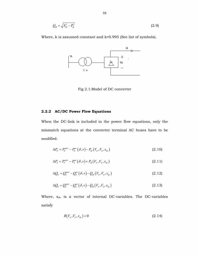
2.2.1 DC System Model
The equations describing the steady state behavior of a mono-polar
DC link (Fig 2.1) can be summarized as follows:
3 2 3cosdr r tr r c dV a V X Iαπ π
= − (2.1)
3 2 3cosdi i ti i c dV aV X Iγπ π
= − (2.2)
dr di d dV V r I= + (2.3)
dr dr dP V I= (2.4)
di di dP V I= (2.5)
3 2dr r tr dS k a V I
π= (2.6)
3 2di i ti dS k aV I
π= (2.7)
2 2dr dr drQ S P= − (2.8)
59
2 2di di diQ S P= − (2.9)
Where, k is assumed constant and k≈0.995 (See list of symbols).
Fig 2.1:Model of DC converter
2.2.2 AC/DC Power Flow Equations
When the DC-link is included in the power flow equations, only the
mismatch equations at the converter terminal AC buses have to be
modified.
( ) ( ), , ,spec actr tr tr dr tr ti dcP P P v P V V xδ∆ = − − (2.10)
( ) ( ), , ,spec acti ti ti di tr ti dcP P P v P V V xδ∆ = − + (2.11)
( ) ( ), , ,spec actr tr tr dr tr ti dcQ Q Q v Q V V xδ∆ = − − (2.12)
( ) ( ), , ,spec acti ti ti di tr ti dcQ Q Q v Q V V xδ∆ = − − (2.13)
Where, xdc is a vector of internal DC-variables. The DC-variables
satisfy
( ), , 0tr ti dcR V V x = (2.14)
60
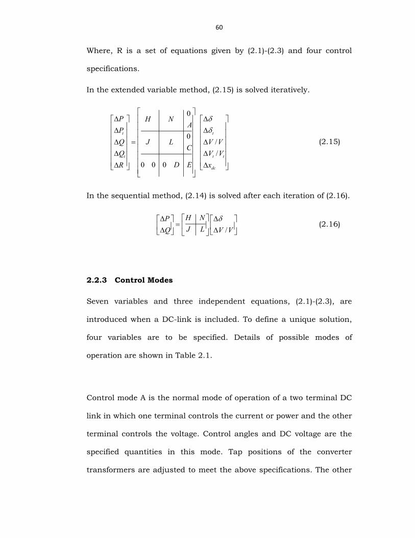
Where, R is a set of equations given by (2.1)-(2.3) and four control
specifications.
In the extended variable method, (2.15) is solved iteratively.
0
0//
0 0 0
t t
t t t
dc
P H NA
PQ J L V V
CQ V V
D ER x
δδ
∆ ∆ ∆ ∆ ∆ = ∆ ∆ ∆ ∆ ∆
(2.15)
In the sequential method, (2.14) is solved after each iteration of (2.16).
/
H NPJ LQ V V
δ ∆ ∆ = ∆ ∆
(2.16)
2.2.3 Control Modes
Seven variables and three independent equations, (2.1)-(2.3), are
introduced when a DC-link is included. To define a unique solution,
four variables are to be specified. Details of possible modes of
operation are shown in Table 2.1.
Control mode A is the normal mode of operation of a two terminal DC
link in which one terminal controls the current or power and the other
terminal controls the voltage. Control angles and DC voltage are the
specified quantities in this mode. Tap positions of the converter
transformers are adjusted to meet the above specifications. The other
61
modes in Table 2.1 are obtained from mode A if variables hit their
limits during the power flow computations, or if the time scale is such
that the taps can be assumed to be fixed. The possibility of obtaining
new modes when limits are encountered, depend on the control
strategy adopted for the HVDC-scheme and the same must be
incorporated in the computations. For modes B - D, ar determines α r
and ai determines the direct voltage, which normally is the case for
current control in the rectifier. Firing angle of the rectifier determines
the direct voltage for modes E – G. Constant current control is
denoted with subscript I.

62
Table 2.1: Control modes
Control
Mode
Specified
Variables
A rα iγ diV diP
B ra iγ diV diP
C rα iγ ia diP
D ra iγ ia diP
E rα iγ ra diP
F rα ia diV diP
G rα ia ra diP
AI rα iγ diV dI
BI ra iγ diV dI
CI rα iγ ia dI
DI ra iγ ia dI
EI rα iγ ra dI
FI rα ia diV dI
GI rα ia ra dI
63
Initially, discrete tap positions are considered by assuming the taps to
be continuous and at a later stage the taps are fixed at appropriate
values.
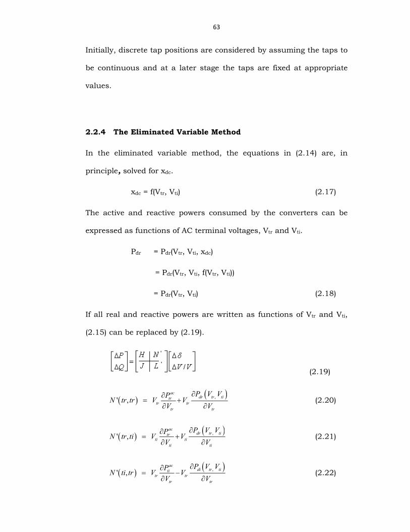
2.2.4 The Eliminated Variable Method
In the eliminated variable method, the equations in (2.14) are, in
principle, solved for xdc.
xdc = f(Vtr, Vti) (2.17)
The active and reactive powers consumed by the converters can be
expressed as functions of AC terminal voltages, Vtr and Vti.
Pdr = Pdr(Vtr, Vti, xdc)
= Pdr(Vtr, Vti, f(Vtr, Vti))
= Pdr(Vtr, Vti) (2.18)
If all real and reactive powers are written as functions of Vtr and Vti,
(2.15) can be replaced by (2.19).
(2.19)
( ) ( ),' ,ac
dr tr titrtr tr
tr tr
P V VPN tr tr V VV V
∂∂= +
∂ ∂ (2.20)
( ) ( ),' ,ac
dr tr titrti ti
ti ti
P V VPN tr ti V VV V
∂∂= +
∂ ∂ (2.21)
( ) ( ),' ,ac
di tr tititr tr
tr tr
P V VPN ti tr V VV V
∂∂= −
∂ ∂ (2.22)
64
( ) ( ),' ,ac
di tr tititi ti
ti ti
P V VPN ti ti V VV V
∂∂= −
∂ ∂ (2.23)
'L is modified analogously. In the eliminated variable method, when a
DC-link is included in the power flow, four mismatch equations and
upto eight elements of the Jacobian have to be changed. Also the DC
variables are not included in the solution vector. The partial
derivatives required by (2.19); eg., ∂Pdr(Vtr,Vti)/∂Vtr is the derivative of
Pdr w.r.t. Vtr, assuming Vti as constant. The DC variables, however, are
not kept constant as opposed to ∂Pdr(Vtr,Vti,xdc)/∂Vtr, which is used in
(2.15). Although (2.19) looks like (2.16), it is mathematically more
similar to (2.15). The Jacobean in (2.19) is well-conditioned than the
one in (2.15).
2.2.5 Analytical Elimination
To illustrate the procedure, the analytical elimination is carried out in
detail for some representative modes. It is sufficient to find Pd and Sd
at each converter, since Qd can be computed with (2.8) or (2.9).
Control Mode A: [αr γi Vdi Pdi]
Since both the voltage and power at the inverter are specified, the
direct current can be computed with (2.5), and Pdr can then be found
by combining (2.3), (2.4) and (2.5).
Pdr = Pdi + Rd Id2 (2.24)
65
If we combine (2.l), (2.6) and (2.24), we obtain
23
cos
di d c d
drr
P R X IS k π
α
+ + =
( )di l lk P P Qα= + + (2.25)
Analogously, for Sdi:
( ) ( )cosdi di l di l
i
kS P Q k P Qγγ= + = + (2.26)
Thus, all real and reactive powers consumed by the converters can be
pre-computed, and including the dc-link in the power flow is trivial for
this control mode. The same is true for any specification of the form
[αr γi x1 x2], where x1 and x2 are any two variables of [Pdr Pdi Vdr Vdi
Id].
Control Mode B: [αr γi Vdi Pdi]
This mode occurs if the tap changer at the rectifier hits a limit in
control mode A under current control in the rectifier. Since Pdi and Vdi
are specified, Id, Vdr, Pdr and Sdi are computed as for mode A. Since αr
is specified, Sdr is computed with (2.6) instead of (2.25).
3 2drtr tr r d dr
tr
SV V k a I SV π
∂= = ∂
(2.27)
2dr dr
trtr dr
Q SVV Q
∂=
∂ (2.28)
66
The formulas for mode BI are identical; the only difference is that Pdi,
rather than Id, is computed with (2.5). In general, when two of the
variables of [Pdr Pdi Vdr Vdi Id] are specified, the other three can be
computed from (2.3)-(2.5).
Control Mode C: [αr γi ai Pdi]
These specifications are valid e.g. if the tap changer at the inverter
hits a limit in mode A under current control in the rectifier.
Combining (2.2) and (2.5) gives
23 2 3cosdi i ti i d c dP a V I X Iγπ π
= − (2.29)
If we solve for Id, we obtain ( )21 1 2d ti ti diI c V c V c P= − − (2.30)
( )
21
1 21 2
d ti
ti ti di
I c VcV c V c P
∂= −
∂ − (2.31)
Where, 1cos2
i i
c
acXγ
= (2.32)
2 3 c
cXπ
= (2.33)
Define ∂Ii as
ti di
d ti
V III V
∂∂ =
∂ (2.34)
Since Pdi is specified, both its partials are zero. Pdr is given by (2.24),
and its partial derivatives by:
67
0drtr
tr
PVV∂
=∂
(2.35)
22 2dr ti dti d d l i
ti d ti
P V IV R I P IV I V∂ ∂
= = ∂∂ ∂
(2.36)
Since ia is specified, Sdi is computed with (2.7), and the partial
derivatives of Qdi are given by:
0ditr
tr
QVV
∂=
∂ (2.37)
( )2
1di diti i
ti di
Q SV IV Q
∂= +∂
∂ (2.38)
Qdr and its partial derivatives are computed from (2.25).
( )2drti i l l
ti
SV I k P QV α
∂= ∂ +
∂ (2.39)
0drtr
tr
QVV
∂=
∂ (2.40)
( )2dr iti dr l l l dr
ti dr
Q IV k S Q P PPV Q α
∂ ∂ = + − ∂ (2.41)
Other Modes
The partial derivatives for the other control modes can be derived
analogously; if the tap changer controlling the control angle is
specified (modes B, D, F, G), only the reactive power at that converter
will depend on corresponding AC voltage. All the active and reactive
powers will depend on the AC voltage at that terminal, if the tap
changer controlling the direct voltage is specified (modes C, D, E, G).

68
Equations (2.30) or (2.43) are used to find the direct current for
constant power control.
If the tap changer position is specified at a converter, Sd is computed
with (2.6) or (2.7), otherwise (2.25) or (2.26) are used. All the eight
partial derivatives for all possible modes listed in Table 2.1 are
summarized in Table 2.2 and Table 2.3.
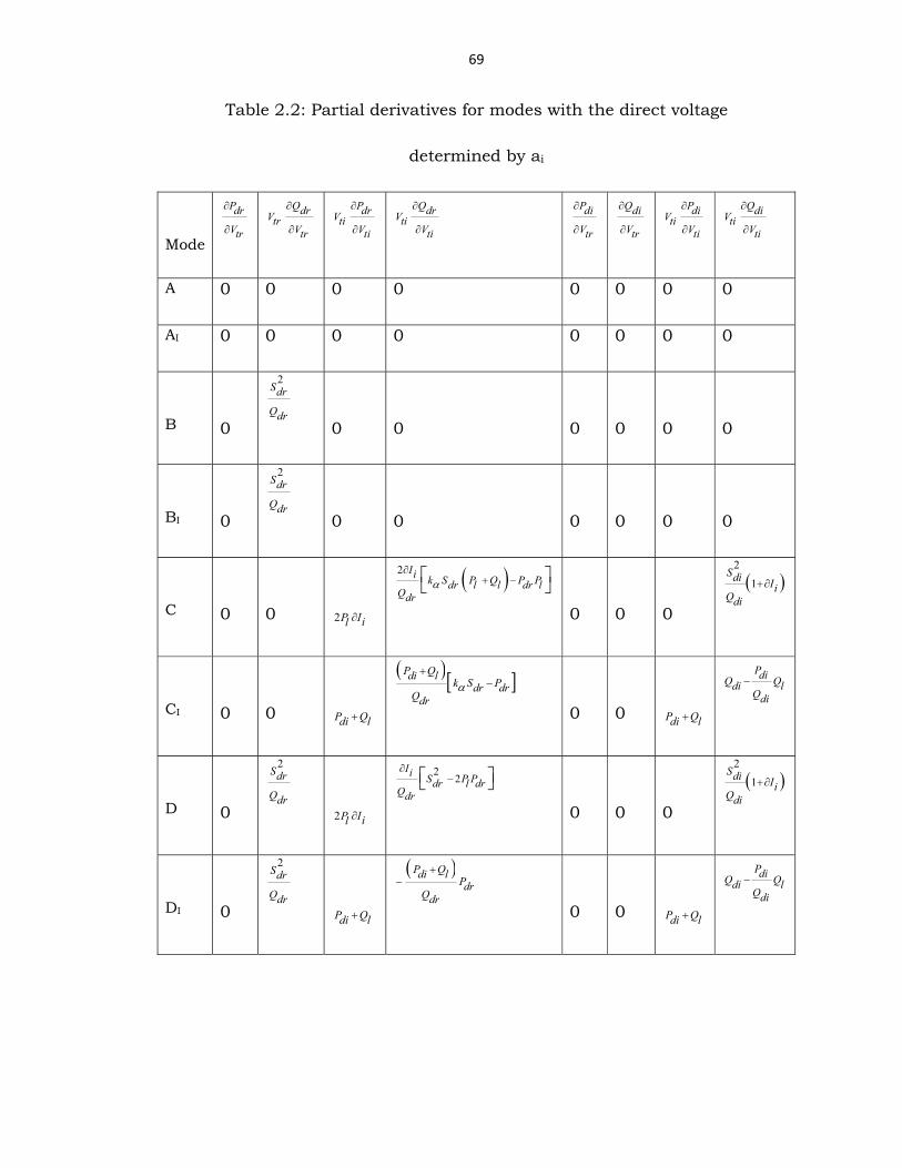
69
Table 2.2: Partial derivatives for modes with the direct voltage
determined by ai
Mode
Pdr
Vtr
∂
∂
QdrVtrVtr
∂
∂
PdrVtiVti
∂
∂
QdrVtiVti
∂
∂
Pdi
Vtr
∂
∂
Qdi
Vtr
∂
∂
PdiVtiVti
∂
∂
QdiVtiVti
∂
∂
A 0 0 0 0 0 0 0 0
AI 0 0 0 0 0 0 0 0
B
0
2Sdr
Qdr
0
0
0
0
0
0
BI
0
2Sdr
Qdr
0
0
0
0
0
0
C
0
0
2P Iil ∂
( )2 Ii k S P Q P Pdr l l dr lQdr
α∂
+ −
0
0
0
( )2
1Sdi IiQdi
+∂
CI
0
0
P Qdi l+
( )[ ]P Qdi l k S Pdr drQdr
α+
−
0
0
P Qdi l+
PdiQ Qdi lQdi
−
D
0
2Sdr
Qdr
2P Iil ∂
22
Ii S P Pdr l drQdr
∂−
0
0
0
( )2
1Sdi IiQdi
+∂
DI
0
2Sdr
Qdr
P Qdi l+
( )P Qdi l PdrQdr
+−
0
0
P Qdi l+
PdiQ Qdi lQdi
−
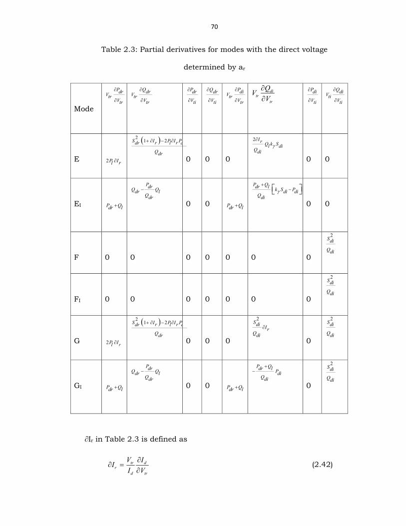
70
Table 2.3: Partial derivatives for modes with the direct voltage
determined by ar
Mode
PdrVtrVtr
∂
∂
QdrVtrVtr
∂
∂
Pdr
Vti
∂
∂
Qdr
Vti
∂
∂
PdiVtrVtr
∂
∂
ditr
tr
QVV
∂∂
Pdi
Vti
∂
∂
QdiVtiVti
∂
∂
E
2P Irl ∂
( )21 2S I P I Pr rdr l d
Qdr
+ ∂ − ∂
0
0
0
2 Ir Q k Sl diQdi
γ∂
0
0
EI
P Qdr l+
PdrQ Qdr lQdr
−
0
0
P Qdr l+
P Qdr l k S Pdi diQdi
γ+
−
0
0
F
0
0
0
0
0
0
0
2Sdi
Qdi
FI
0
0
0
0
0
0
0
2Sdi
Qdi
G
2 rP Il ∂
( )21 2S I P I Pr rdr l d
Qdr
+ ∂ − ∂
0
0
0
2Sdi IrQdi
∂
0
2Sdi
Qdi
GI
P Qdr l+
PdrQ Qdr lQdr
−
0
0
P Qdr l+
P Qdr l PdiQdi
+−
0
2Sdi
Qdi
∂Ir in Table 2.3 is defined as
tr dr
d tr
V III V
∂∂ =
∂ (2.42)

71
Where, ( )23 3 4d tr tr diI c V c V c P= − − (2.43)
( )33 cos
2 3r r
d c
acR X
απ
=+
(2.44)
4 3d c
cR X
ππ
=+
(2.45)
2.3 TRANSIENT STABILITY STUDIES
Transient stability studies provide information related to the capability
of a power system to remain in synchronism during major
disturbances resulting from either the loss of generation or
transmission facilities, sudden or sustained load changes, or
momentary faults [114]. Specifically, these studies provide the
changes in the voltages, currents, powers, speeds, and torques of the
machines of the power system, as well as the changes in system
voltages and power flows, during and immediately following a
disturbance. In the planning of new facilities the degree of stability of
a power system is an important factor. In order to provide the
reliability required by the dependence on continuous electric service,
it is necessary that power systems be designed to be stable under any
conceivable disturbance.
The power system transient performance can be obtained from the
network equations. The performance equation using the bus frame of
reference in either the impedance or admittance form has been used
in transient stability calculations.

72
The operating characteristics of synchronous machines are described
by a set of differential equations. The number of differential equations
required for a machine depends on the details needed to represent
accurately the machine performance.
Transient stability analysis outcome is the resultant solution of the
network algebraic equations and the machine differential equations.
The solution of the network equations retains the identity of the
system and thereby provides access to system voltages and currents
during the transient period.
As compared with rotor long-time constants, the AC and DC-
transmission systems respond rapidly to network and load changes.
The time constants associated with the network variables are
extremely small and can be neglected without significant loss of
accuracy. Also stator time constants of the synchronous machine may
be taken as zero.
The DC link is assumed here to maintain normal operation
throughout the disturbance. This approach is not valid for larger
disturbances such as converter faults, DC-line faults and AC faults
close to the converter stations, these disturbances can cause
commutation failures and alter the normal conduction sequence [105].
73
2.3.1 Generator Representation
The synchronous machine is represented by a voltage source that is
constant in magnitude but changes in angular position, behind its
transient reactance. The effect of saliency is neglected in this
representation and it assumes constant flux linkages and a small
change in speed. If the machine rotor speed is assumed constant at
synchronous speed, then M is constant. The machine accelerating
power is equal to the difference between the mechanical power and
the electrical power [6] if the rotational losses are neglected. The
classical model can be described by the following set of differential
and algebraic equations:
Differential:
( )
2
2
2
m e
d fdtd d f P Pdt dt H
δ ω π
δ ω π
= −
= = − (2.46)
Algebraic:
' 't a t d tE E r I jx I= + + (2.47)
Where, E ′=voltage back of transient reactance
Et =machine terminal voltage
It =machine terminal current
ra =armature resistance
'dx =transient reactance

74
Fig 2.2: Generator Classical model
2.3.2 Load Representation
Power system loads, other than motors, can be treated in several ways
during the transient period. The commonly used representations are
either static impedance or admittance to ground, constant real and
reactive power, or a combination of these representations. The
parameters associated with static impedance and constant current
representations are obtained from the load flow solution for the power
system prior to a disturbance. The initial value of the current for a
constant current representation is obtained from
*lp lp
pop
P jQI
E−
= (2.48)
The static admittance Ypo used to represent the load at bus P, can be
obtained from
popo
p
IY
E=
(2.49)
Where, Ep is the calculated bus voltage, Plp and Qlp are the scheduled
real and reactive bus loads. Corresponding to each load bus, using the
75
expression for Ypo discussed above, the diagonal elements of the
admittance matrix are modified.
2.3.3 HVDC System Representation
For the representation of DC systems in stability studies standard
models have not been developed [1], since each DC system tends to
have unique characteristics to meet the specific needs of its
application.
a) Converter model
i) Simplified model
Here valve switching is neglected and the converter is represented by
the average DC voltage equation. This model is similar to that used in
power flow analysis. The transformer tap is assumed to be constant as
the tap changer dynamics are very slow [65]. This model is inaccurate
during severe disturbances such as unsymmetrical faults and cannot
handle commutation failures.
ii) Detailed model
Here, the valve switching is incorporated and the model is free from
the drawbacks associated with the simplified model. However the
transient simulation of converter now requires integration step size as
small as 50 – 100 µs. This implies heavy computation burden, so it is

76
used only for short duration (say 0.2 sec) immediately after the
disturbance.
b) Converter Controller Models
i) Response type model
The dynamics of the CEA and CC are neglected and only the steady –
state controller characteristics are represented. The main feature of
this type of controller model is that the configuration and the
parameters of the controller are assumed to be designed at a later
stage based on the requirement.
ii) Detailed Representation
It requires the analysis of actual control circuitry and the
establishment of a dynamic equivalent with a frequency response
which matches the actual controller response. This is used along with
the detailed converter model.
c) DC Network Model
i) Resistive network
Here DC network is represented as resistive network ignoring energy
storage elements. This approach is valid when DC lines are short and
for back to back HVDC links where the smoothing reactors are of
moderate size.
77
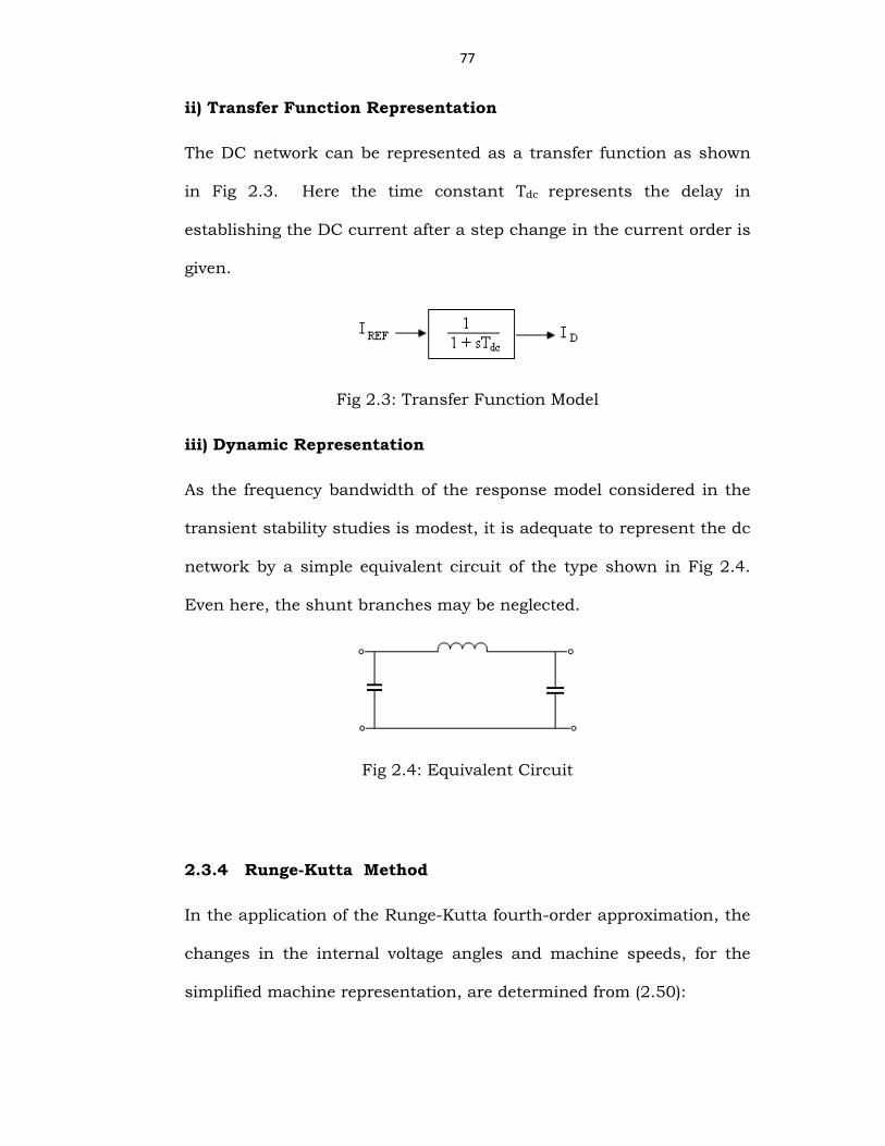
ii) Transfer Function Representation
The DC network can be represented as a transfer function as shown
in Fig 2.3. Here the time constant Tdc represents the delay in
establishing the DC current after a step change in the current order is
given.
Fig 2.3: Transfer Function Model
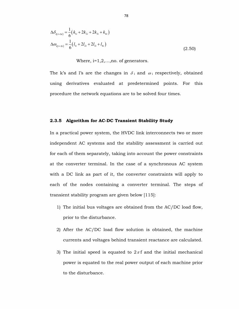
iii) Dynamic Representation
As the frequency bandwidth of the response model considered in the
transient stability studies is modest, it is adequate to represent the dc
network by a simple equivalent circuit of the type shown in Fig 2.4.
Even here, the shunt branches may be neglected.
Fig 2.4: Equivalent Circuit
2.3.4 Runge-Kutta Method
In the application of the Runge-Kutta fourth-order approximation, the
changes in the internal voltage angles and machine speeds, for the
simplified machine representation, are determined from (2.50):
78
( ) ( )
( ) ( )
1 2 3 4
1 2 3 4
1 2 261 2 26
i i i ii t t
i i i ii t t
k k k k
l l l l
δ
ω
+∆
+∆
∆ = + + +
∆ = + + + (2.50)
Where, i=1,2,…,no. of generators.
The k’s and l’s are the changes in δ i and ω i respectively, obtained
using derivatives evaluated at predetermined points. For this
procedure the network equations are to be solved four times.
2.3.5 Algorithm for AC-DC Transient Stability Study
In a practical power system, the HVDC link interconnects two or more
independent AC systems and the stability assessment is carried out
for each of them separately, taking into account the power constraints
at the converter terminal. In the case of a synchronous AC system
with a DC link as part of it, the converter constraints will apply to
each of the nodes containing a converter terminal. The steps of
transient stability program are given below [115]:
1) The initial bus voltages are obtained from the AC/DC load flow,
prior to the disturbance.
2) After the AC/DC load flow solution is obtained, the machine
currents and voltages behind transient reactance are calculated.
3) The initial speed is equated to 2π f and the initial mechanical
power is equated to the real power output of each machine prior
to the disturbance.
79
4) The network data is modified for the new representation. Extra
nodes are added to represent the generator internal voltages.
Admittance matrix is modified to incorporate the load
representation.
5) Set time, t=0.
6) For any switching operation or change in fault condition,
network data is to be modified accordingly and the AC/DC load
flow is to be performed.
7) Machine differential equations are to be solved using Runge-
Kutta method to find the changes in the internal voltage angles
and machine speeds.
8) Internal voltage angles and machine speeds are to be updated
and stored for plotting.
9) AC/DC load flow is to be performed again to get the new output
powers of the machines.
10)Advance time, t=t+∆t.
11) Check for time limit. If t ≤ tmax repeat the process from step 6,
else plot the graphs of internal voltage angle variations and stop
the process.

80
From the plots obtained using the procedure detailed above, it can be
judged whether the system is stable or unstable. For the analysis of
multi machine system stability, the plot of relative angles is to be
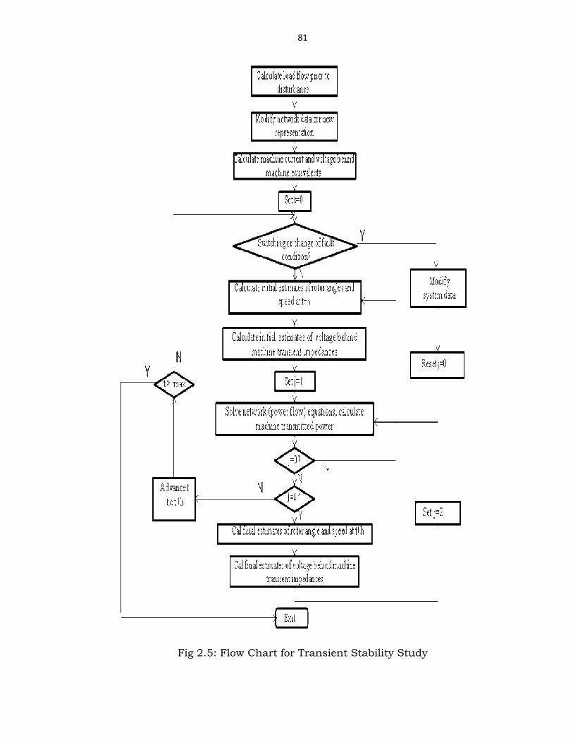
evaluated. The flow chart for transient stability study depicting the
above algorithm is given in Fig 2.5.
81
Fig 2.5: Flow Chart for Transient Stability Study

82
The transient stability analysis detailed above is initially applied for a
Single Machine Infinite bus system with parallel AC & DC links and
then for a typical Multi Machine System with a single DC link and
these are detailed in the subsequent chapters.