chapter 2 literature - um
TRANSCRIPT
24
CHAPTER 2
LITERATURE REVIEW
The previous chapter highlighted the need for a relevant valuation model to calculate
the cost of equity for the Malaysian firms. Based on the studies on practitioners’
preference for various techniques to calculate cost of equity, it has come to our attention
that the CAPM is the most popular model among practitioners in developed as well as
in emerging markets. Therefore, the current chapter is devoted to review past studies on
the CAPM, starting with the introduction of the CAPM in the 1960s, the critics on the
model, the variations of the CAPM resulting from attempts to overcome the original
model’s weaknesses and the adoptions on the CAPM for the emerging markets. In the
last section, we dwell into studies related to cost of equity determinants.
2.1 CAPM and Cost of Equity Calculation
A firm’s cost of equity represents the compensation that investor demands in substitute
for bearing the risks that come with owning the firm’s common stocks. Being risk
adverse, it is assumed that investors require a risk premium for additional risk on top of
a risk-free return. It is easy to understand why the CAPM is popular among practitioner,
as the CAPM is the basic theory that conveniently links risks and returns for all risky
assets.
CAPM was the work of William Sharpe, a Nobel laureate in economics, that was set out
in his book entitled “Portfolio Theory and Capital Markets” in 1970. The main idea
behind his model is that not all risks should affect asset prices. Therefore, individual
investment contains two types of risk, systematic risk and unsystematic risk. Systematic
risk is market risk that cannot be diversified away and this risk affects almost all stocks.

25
Examples are changes in interest rates, economy recessions and wars. On the other hand,
unsystematic risk is risk specific to individual firms or stocks that can be eliminated as
investors increase the number of stocks in their portfolios. Some examples include
product defects or an announcement on a merger of firms. Modern portfolio theory
shows that unsystematic risk can be eliminated through diversification. Nevertheless,
diversification does not solve the problem of systematic risk, that is, it cannot eliminate
systematic risk. Therefore, when calculating expected return, systematic risk is what
troubles investors most. The CAPM, hence, is created as a model that allows estimation
of this systematic risk.
An important component of the CAPM is the risk-free rate. To this, a premium is added
for additional risk that investors have to bear. The premium consists of a market risk
premium multiplied by a coefficient called beta. Beta, when compared to the market
risk premium, indicates the amount of compensation needed for investors to take on
additional risks. Therefore, there are basically three inputs to the CAPM framework that
need to be estimated – risk-free rate, firm’s beta and market risk premium. Among the
trio, the risk-free rate is the least controversial estimate one has to make. There are
nevertheless, two issues to be considered. First, what constitute a good risk-free rate,
and second, which maturity should be used for the risk-free rate? Since there are no
assets that are really risk-free, it is a norm to use Treasury securities to represent the
risk-free asset. As a general rule of thumb, the maturity chosen for the risk-free rate
should match the maturity of the project under valuation. Nevertheless, most finance
textbooks suggest using short-term rates since they are consistent with simplest version
of the CAPM (Titman et al., 2008, p. 138).
26
The second estimate in the CAPM is firm’s beta or simply known as beta, which
measures the sensitivity of stock returns relative to market returns. The basic concept of
beta arises because stock returns tend to move in tandem with the movement of the
overall market returns to a certain extent. Some may move more than others or could
move in the same or opposite direction to the movement of the overall market.
Therefore, their sensitivity to the overall market movements is an important measure.
As market itself has a beta of 1.0, a firm whose stock returns that vary more than the
market will have an absolute value of greater than 1.0. On the other hand, a firm whose
stock returns vary less than the market will have an absolute beta value of less than 1.0.
Since beta takes into account direction and magnitude, a beta of say 1.5 indicates that if
the market returns go up ten percent, the stock returns will go up 15 percent. However,
if the beta value is negative, then stock returns will move in the opposite direction of the
market returns. A beta can be estimated through the market model regression whereby
stock returns are regressed against market returns.
The last input for the CAPM is the equity risk premium for the market. To obtain the
estimate, the difference between long-run historical rates of return of the market and the
rates of return from a risk-free investment is conventionally used. The assumption is
that historical data can be used to forecast equity risk premiums in the future. To obtain
cost of equity estimates for firms, the estimation of the equity risk premium is the most
controversial and difficult. There have been arguments of whether equity risk premium
observed in practice is compatible with theory. In their seminar paper, Mehra and
Prescott (1985) argued that the observed historical equity risk premiums in the U.S. are
much higher than could be justified by standard theory and it would take implausibly
high risk-aversion investors to demand these premiums. They termed it as the “equity
premium puzzle”. Since then, numerous studies have attempted to provide plausible
27
explanations to the puzzle but no consensus has been reached yet. This has led some
researchers to believe that the logical explanations to the puzzle are either the standard
models are wrong or historical risk premium is misleading (Dimson et al., 2008).
Indeed, Damodaran (2010) concluded that it is not clear what to make of the equity
premium puzzle. He added that the puzzle highlighted more on the danger of using
historical data and the failure of classic utility models than of the equity risk premium
itself.
Standard procedure for estimating equity risk premium is to use the historical risk
premium approach, whereby the historical returns earned by stocks above the risk-free
rate over a long period are employed. However, Damodaran (2008) argued that while
the approach may yield reasonable estimates for countries with a large and diversified
stock market which has a long history and a well developed government bond market
like the U.S., the approach yield meaningless estimates for the emerging markets where
the equity market represents a small proportion of the overall economy and historical
data tend to be limited and noisy.3 He suggested the use of a base premium for a mature
equity market such as the U.S. and a country risk premium to estimate equity risk
premium.
To measure country risk premium, Damodaran (2008) suggested using the rating
assigned to a country’s debt by a rating agency like the S&P and Moody’s. The
advantage of these ratings is that although they measure default risk rather than equity
risk, they are affected by many of the factors which drive equity risk as well. Some of
the factors include political stability, currency fluctuation and trade balances. Indeed,
Pereiro (2001) found that very short time series in volatile settings has caused some
3 The paper has gone through a few revisions. It seems that an early draft of the paper has been available since as early as year 2000, as quoted in Pereiro (2001).
28
Latin American countries such as Chile, Colombia and Peru to have negative market
risk premiums. He mentioned that a solution for the problem may be to apply the
sovereign bond premium introduced by Damodaran.
After linking the CAPM to the calculation of cost of equity, the following two sub-
sections contain further discussion of the CAPM. In particular, the assumptions of and
critics on the model, as well as extensions of the model aimed to modify or relax its
simplified assumptions are discussed.
2.1.1 Assumptions and Critics of the CAPM
A massive amount of research had been devoted to the empirical testing of the CAPM
over the several past decades. Nevertheless, the empirical evidence supporting the
model was poor. Fama and French (2004) attributed the lack of empirical support to the
simplifying assumptions underlying the model. Adapted from Elton et al. (2007, p. 285),
the CAPM is based on the framework of an efficient market with the following
assumptions:
i) No transaction costs. There is no cost involved in buying or selling any asset.
The inclusion of transaction cost adds a great deal of complexity to the
model.
ii) Assets are infinitely divisible. Investors are able to take any position in an
investment.
iii) No personal income tax. Investors are indifferent whether to receive the
return on their investment in the form of dividends or capital gains.
iv) Perfect competition. Individual cannot affect the stock price by his/her
buying or selling action, that is, all investors are price takers.
29
v) Investors are expected to make decisions solely in terms of expected values
and standard deviations of the returns on their portfolios.
vi) Unlimited short sales.
vii) Unlimited lending and borrowing at the riskless rate.
viii) Investors are assumed to be concerned with the mean and variance of returns
(or prices over a single period), and are assumed to define the relevant
period for investment in exactly the same manner.
ix) Investors are assumed to have identical expectations with respect to the
necessary inputs for making portfolio decisions, that is, expected returns,
variance of returns and the correlation structure between all pairs of stocks.
x) All assets, including human capital are marketable. It is assumed that the
market portfolio consists of all types of assets, including works of art, real
estate, human capital and so on.
It is obvious that many of these assumptions do not hold in the real world and one might
find the assumptions behind the CAPM unrealistic. There were various critiques on the
CAPM but the most famous is none other than Roll’s (1977) critique.
Roll’s critique is a famous analysis of the validity of the empirical test of CAPM. In his
paper, two statements were made regarding the market portfolio. The first statement is
the mean-variance tautology. He argued that the validity of the CAPM is equivalent to
the market being mean-variance efficient with respect to all investment opportunities.
Without observing all investment opportunities, it is not possible to test whether a
portfolio is mean-variance efficient. Consequently, it is not possible to test the CAPM.
The second statement is made with regards to the unobservable market portfolio. He
argued that the market portfolio in practice would necessarily include every single
30
possible available asset, including real asset, precious metals, stamp collections,
jewellery, and anything with any worth. The returns on all possible investment
opportunities are unobservable. Roll's critique has received a large number of citations
in the financial economics literature but it is the second statement that is mostly cited.
Hence, it is not surprising that Roll’s critique is interpreted as “the market portfolio is
unobservable’.
2.1.2 Extensions of the CAPM
Attempts to modify or relax most of the assumptions of the CAPM have resulted in
variations of the traditional CAPM model. Some of the prominent extensions include
eliminating the possibility of unlimited lending and borrowing at a riskless rate
(Brennan, 1971; Black, 1972), allowing some assets to be nonmarketable (Mayers,
1973), having heterogeneous expectations (Lintner, 1969; Gonedes, 1976), presence of
personal taxes (Elton and Gruber, 1978) and allowing for multi-period and changing
investment opportunities from one period to another (multi-beta model by Merton
(1973), consumption CAPM by Breeden (1979); inflation CAPM by Friend et al.
(1976)). Despite the changes in assumptions, many of the conclusions of the original
CAPM remain the same. This shows that the simple form of the CAPM is amazingly
robust (Elton et al., 2007, p. 324).
Another strand of the extension to CAPM stems from the findings that variation in
average stock returns could not be fully explained by market beta. Basu (1977) found
that low price-to-earnings ratios to be associated with higher rates of return than what
could be explained by the CAPM, Banz (1981) and Reinganum (1981) showed that this
price-to-earnings effect was related to firm size, while Litzenberger and Ramaswamy
(1982) found that higher stock returns are associated with high dividend yields. The

31
ability of other risk factors in explaining stock returns has motivated researchers to
examine the performance of alternative models that explain stock returns better. Based
on the asset pricing literature, these alternative models take three separate directions,
which are (i) multifactor models that add some factors to the market return, (ii) the
Arbitrage Pricing Model (APT) of Ross (1976), and (iii) the incorporation of higher
moments such as skewness and kurtosis.
The most prominent multifactor model is perhaps the one introduced by Fama and
French (1993). Their three-factor (FF3F) CAPM model showed that by adding a ‘value’
(book-to-market equity) factor and a ‘size’ (firm size) factor on top of the overall
market factor greatly improves the explanatory power of the CAPM on stock returns. In
their observation, small firms and stocks with high book-to-market ratio tend to do
better than the overall market. Later, Fama and French (1996) found that the FF3F is
also able to explain the strong patterns in returns observed when portfolios are formed
on earnings-to-price ratio, cash flow-to-price ratio, and sales growth. Despite this, the
FF3F was found to leave many other important anomalies unexplained. One of such
anomalies is Jegadeesh and Titman’s (1993) momentum effect. They found stocks that
do well in the past three to 12-month holding periods tend to do well in the next few
months and stocks that do not do well will continue to perform poorly. An alternative
approach will be to apply Carhart (1997) four-factor model whereby momentum is
added as the fourth factor to the FF3F to take into account the persistency in short-term
returns. Nonetheless, due to the short-lived nature of the momentum effect, it is
irrelevant in cost of equity estimation (Fama and French, 2004).
Recent empirical findings showed that FF3F has limited explanatory power on stock
returns. For example, Martinez et al. (2005) showed that the FF3F has limited

32
explanatory power on cross-sectional expected stock returns in the Spanish market. Liu
(2006) also shared similar findings for the NYSE, AMEX and NASDAQ markets. In
particular, the FF3F is criticised for failing to capture liquidity risk. In Liu’s study, it is
shown that liquidity risk is priced and is important for asset pricing. The survey by
Bruner et al. (1998) revealed that only a minority of firms used multi-factor asset
pricing models to estimate cost of equity. Ang et al. (2006) also demonstrated that only
the market factor is consistently priced for 23 developed markets over a sample period
of 1980-2003. Interestingly, size, book-to-market, momentum and liquidity are not able
to account for the low average returns earned by stocks with high systematic risk.
The APT developed by Ross (1976) serves many of the same functions as the CAPM
but has more flexibility because the model does not require the benchmark market
portfolio to be the unobservable ‘market’ portfolio. In addition, the APT suggests that
there are factors other than beta which affect systematic risk. Since the APT does not
clearly specify the risk factors, the model opens up to many possible sources of risk and
uncertainty. Motivated by the APT, Chen et al. (1986) managed to identify a set of
macroeconomic variables, which in their view, explained expected returns. They are
industrial production, risk premium, term structure of interest rates, and inflation. While
they do not claim to have found the “true” set of variables for asset pricing, the paper
has since motivated a series of research of this sort, see for example, Burmeister and
Wall (1986), Burmeister and McElroy (1988), Chen and Jordan (1993), and Shanken
and Weinstein (2006).
Although APT seems to be an extremely appealing model, the large macroeconomic
data series required become a drawback of the model, especially in emerging markets
where the data are usually incomplete, extremely short and very volatile. This may
33
explain why APT is less popular for applications in less developed markets. As stated in
Pereiro (2002, p. 110) “In Argentina, it has been shown that only eight percent of the
corporations and none of the private equity funds or financial advisors surveyed use
APT models when computing the cost-of-equity capital...”. In addition, the lack of
agreement among practitioners and academics regarding risk factors has limited the
applications of APT (Ameer, 2007).
The third category of studies pays attention to the third- and fourth-order moments of
return distribution, that is, skewness and kurtosis, respectively. Arditti (1971) argued
that investors do not base their decisions solely on the first two-moments on the return
probability distributions, but show a preference for positive skewness. Kraus and
Litzenberger (1976) extended the two-moment CAPM to include the effect of positive
preference for skewness. They documented that the three-moment CAPM is a better
predictor of stock returns than its two-moment counterpart. Employing sample
consisting of all stocks listed in the NYSE from 1969 to 1988, Fang and Lai (1997)
derived a four-moment CAPM and revealed that conditional skewness and conditional
kurtosis contribute to the risk premium of a stock. Dittmar (2002) improved the CAPM
model by adding the terms for skewness and kurtosis, and found that multi-factor
models lose their significance in explaining cross-sectional of stock returns. Their
results propose that forecasting power may improve when skewness and kurtosis are
included in a model. Nevertheless, some researchers claim that the opposite might be
true (Nagel et al., 2007).
In a recent study, Nagel et al. (2007) compared six commonly used methods in cost of
equity estimation, namely, the CAPM, the FF3F model, the Carhart (1997) four-factor
model, a co-skewness model, a co-kurtosis model and the stock’s own historical mean
34
return. The model in Lee et al. (1999) is used as the base model. Following the base
model, the cost of equity is calculated as the sum of the risk-free rate and a risk
premium averaged over many years. The six mainstream models were built upon the
base model. Using firm sample of all non-financial stock returns available in the Center
for Research in Security Prices (CRSP) from 1953 to 1996, Nagel et al. (2007) found
that the more sophisticated models do not offer forecasting ability more superior than
the base model. They concluded that forecast error from estimating factor loadings and
expected risk premium in the more sophisticated models exceeds the precision gained
by including those risk factors.
In sum, multifactor models emerged as a result of the failure of market beta to explain
cross-sectional variations in stock returns. These models incorporate fundamental
factors such as size and price-to-earnings ratio in addition to the market beta. The non-
normality of stock returns especially in high-frequency data as shown by several studies
resulted in the alternative of CAPM with higher order co-moments. Over the years, the
simple form of the CAPM model has gone through various modifications in adjacent to
new empirical findings. Not only that, as the world globalizes and investors gain access
to foreign investments, other issues emerge and research continues to find a model that
will better grasp the conditions of these markets. With the rapid pace of globalization,
some believe that the world has become more integrated than before and thus one only
need a single asset pricing model to estimate cost of equity. This is discussed in Section
2.2. Section 2.3 will focus on another issue, which is cost of equity estimation for
emerging markets.
35
2.2 Global Cost of Equity
Towards the end of War World II, capital markets around the world were very much
segmented due to the numerous barriers to free flow of capital. The reformation and
liberalization in the developed markets in the 1970s and emerging markets in the 1980s
led to the removal of many of these barriers. Parallel with globalization, the world
capital markets have become more integrated and perhaps a single model is all that one
needs to estimate cost of equity.
In the classic CAPM, investors are assumed to care about only one risk factor – the
overall market risk. How risky is a stock compared to the overall market is captured by
the covariance of the stock returns with the overall market returns, in other words, the
beta for the stock. The discount rate is based on the multiplication of this beta with the
equity risk premium, given as the excess return of the overall market portfolio over the
risk-free rate. Investors evaluating a stock in their own country will probably use the
excess return of the local market portfolio over the local risk-free rate to estimate cost
of equity. However, in today’s globalized market, investors are faced with the question
of whether a global market risk premium should be used instead.
Stehle (1977) and Stulz (1995) argued that the use of a local market index is only
appropriate for closed, national markets. Their reports provide empirical support for the
global CAPM over the local CAPM. On the other hand, Solnik (1974) raised his doubts
that a single global index would give a realistic description of the international context
because national factors are important too. Stulz (1981b) constructed an international
asset pricing model with investment barriers and found that these barriers reduce trade
in assets which do not provide expected returns large enough to offset the cost of
barriers. Accordingly, he concluded that, when there are international investment
36
barriers, the world portfolio of stocks cannot be efficient for any investor. The empirical
evidence seems to suggest the use of a local asset pricing model for segmented markets
while a global asset pricing model for integrated markets.
Perhaps, the more important question here is whether local and global pricing models
will lead to different cost of equity estimates. Empirical evidence on the issue is mixed.
Among the first to address the problem is Stulz (1995). Using the case of the Swiss
multinational Nestlé, he replaced the local market index in the traditional CAPM with a
global market index and showed the difference in cost of equity estimates is about 150
basis points. Mishra and O’Brien (2001) took it a step further by including a third model,
a global CAPM with one additional factor for exchange rate risk, and compared it to the
local CAPM and the global CAPM proposed by Stulz (1995). Unlike Stulz who
examined a single firm, their study included a large sample of equities which is
inclusive of 2989 U.S. stocks and 118 American Depository Receipts (ADRs). They
found the models, on average, do not produce substantial difference in cost of equity
estimates. Koedijk et al. (2002), Harris et al. (2003), and Koedijk and van Dijk (2004)
also shared the view that the local CAPM does not lead to significantly different cost of
equity estimates than those of the global CAPM.
A recent test on the effectiveness of global models in pricing the cross-sectional
emerging market stock returns was done by Barclay et al. (2010). Focusing on monthly
return data for 20 emerging markets (Malaysia inclusive) covering the period of 1995-
2008, eight asset pricing models were tested in the study. The first four models were
unconditional models consisting of (i) simple CAPM with developed world index, (ii)
simple CAPM with emerging world index, (iii) currency model with developed world
index and three currency factors (German Deutsche Mark, Japanese Yen and U.K.
37
Pound Sterling) and (iv) currency model with emerging world index and three currency
factors. The remaining models were conditional models, estimated by adding a global
information variable as a separate factor to each model. They found a wide spread
performance across the eight models in terms of R2, but in general, the conditional
models performed better than the unconditional models. Models factoring in currency
risk have better performance than the single factor models. Nevertheless, when model
misspecification was allowed, the difference in R2 became not significant. An important
implication from the findings is that when controlling for model misspecification, none
of the models outperform the global CAPM.
A drawback of the global CAPM is the assumption that every investor trades using the
same currency. In reality, the investor population around the world are heterogeneous,
coming from different countries and holding different currencies. If the heterogeneity is
taken into account, the model should include additional terms. One of such terms is
exchange rate risk. Some of the earlier studies to incorporate this risk in international
asset pricing are Solnik (1974), Stulz (1981a), and Adler and Dumas (1983).
Nonetheless, currency exchange risk premiums are often much smaller than world
market risk premium (Bodnar et al.,2003) and there is overwhelming evidence that
shows that the covariance between stock returns and exchange rate movements is quite
small (Solnik, 1999, p. 227 as quoted in Pereiro 2001). Other studies, for example,
Hamao (1988) and Jorion (1991), found no evidence that exchange risk is priced in the
Japanese and the U.S. stock market, respectively. However, Pereiro (2001) indicated
that the global CAPM may be plausible for developed markets but certainly not for
emerging markets where country risk is present.
38
2.3 Cost of Equity Estimation in Emerging Market
Despite considerable history of research on emerging markets, much of the current
work was initiated as a result of the World Bank Conference on Portfolio Investment in
Developing Countries, held in Washington in late 1993. Some of the ideas presented at
the conference motivated much of the research on emerging markets over the next five
years. Among the goal of the conference was to think about ‘best practice’ in the issue
of assets valuation in emerging markets and to explore new research and practical
methodologies. One of the most pressing problems professional firm appraisers face in
cost of equity valuation in emerging market is the availability of accurate reliable
information. Empirical evidence shows that emerging equity market information tends
to be scarce and unreliable. Not only that, financial efficiency of emerging markets is
also highly debatable. These are relevant problems, because traditional valuation
techniques including DCF work best when applied to the valuation of stocks of large
public firms, which operate within highly efficient markets in developed economies.
2.3.1 Challenges of Using CAPM in Emerging Market
The first challenge faced by researchers is associated with emerging markets’ imperfect,
incomplete, or short-lived data. Most empirical research on emerging markets relies on
the International Finance Corporation (IFC) indices which represent portfolios of
securities that comprise at least 60 percent of the market capitalization in each emerging
market. For some countries, there are only a few stocks in the IFC index portfolio. For
example in December 1997, emerging countries like Hungary and Venezuela have less
than 20 securities in the IFC global index. India had more than 5,000 equity securities
listed in the country but only 133 securities are included in IFC index. The small
number of securities in these indices means that the country portfolio may contain some
variance that is usually diversified away with larger portfolios. Not only that, empirical
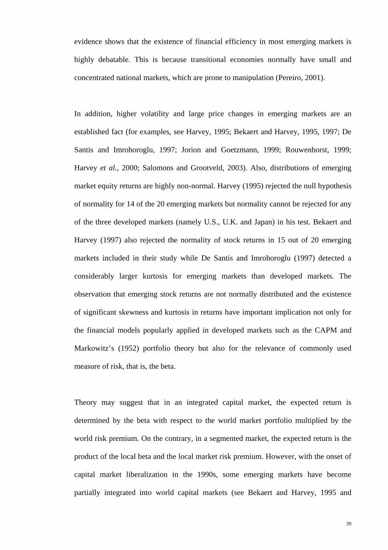
39
evidence shows that the existence of financial efficiency in most emerging markets is
highly debatable. This is because transitional economies normally have small and
concentrated national markets, which are prone to manipulation (Pereiro, 2001).
In addition, higher volatility and large price changes in emerging markets are an
established fact (for examples, see Harvey, 1995; Bekaert and Harvey, 1995, 1997; De
Santis and Imrohoroglu, 1997; Jorion and Goetzmann, 1999; Rouwenhorst, 1999;
Harvey et al., 2000; Salomons and Grootveld, 2003). Also, distributions of emerging
market equity returns are highly non-normal. Harvey (1995) rejected the null hypothesis
of normality for 14 of the 20 emerging markets but normality cannot be rejected for any
of the three developed markets (namely U.S., U.K. and Japan) in his test. Bekaert and
Harvey (1997) also rejected the normality of stock returns in 15 out of 20 emerging
markets included in their study while De Santis and Imrohoroglu (1997) detected a
considerably larger kurtosis for emerging markets than developed markets. The
observation that emerging stock returns are not normally distributed and the existence
of significant skewness and kurtosis in returns have important implication not only for
the financial models popularly applied in developed markets such as the CAPM and
Markowitz’s (1952) portfolio theory but also for the relevance of commonly used
measure of risk, that is, the beta.
Theory may suggest that in an integrated capital market, the expected return is
determined by the beta with respect to the world market portfolio multiplied by the
world risk premium. On the contrary, in a segmented market, the expected return is the
product of the local beta and the local market risk premium. However, with the onset of
capital market liberalization in the 1990s, some emerging markets have become
partially integrated into world capital markets (see Bekaert and Harvey, 1995 and
40
Bekaert et al. 2005). When considering the risk exposure in a market, it is important to
consider the level of market integration. In fully integrated markets, the common factor
with which risk is priced is the covariance of market returns with the world market
portfolio returns. The other extreme is the perfectly segmented market, where market
returns move independently of the world market. In this scenario, the relevant factor
will be the assets’ exposure to factors specific to the segmented market. As emerging
markets lie within the continuum of full integration on one end and full segmentation on
the other end, one would need to consider appropriate risk measures that can capture the
dynamic risk-return relationship in transitional economies.
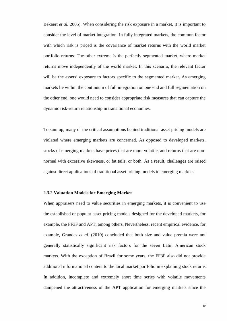
To sum up, many of the critical assumptions behind traditional asset pricing models are
violated where emerging markets are concerned. As opposed to developed markets,
stocks of emerging markets have prices that are more volatile, and returns that are non-
normal with excessive skewness, or fat tails, or both. As a result, challenges are raised
against direct applications of traditional asset pricing models to emerging markets.
2.3.2 Valuation Models for Emerging Market
When appraisers need to value securities in emerging markets, it is convenient to use
the established or popular asset pricing models designed for the developed markets, for
example, the FF3F and APT, among others. Nevertheless, recent empirical evidence, for
example, Grandes et al. (2010) concluded that both size and value premia were not
generally statistically significant risk factors for the seven Latin American stock
markets. With the exception of Brazil for some years, the FF3F also did not provide
additional informational content to the local market portfolio in explaining stock returns.
In addition, incomplete and extremely short time series with volatile movements
dampened the attractiveness of the APT application for emerging markets since the

41
model requires large macroeconomic data series. Not only that, consensus has not been
reached among practitioners and academics regarding the risk factors to be used in the
APT. This has limited the use of the model for emerging markets.
The application of the traditional one-factor CAPM to emerging markets is a
controversial venture. Despite that, Pereiro (2002) felt that chances were, the model will
continue to be used for many years to come and he listed three reasons. First, the
availability of data for easy application of the CAPM model may entice analysts to
continue using it for cost-benefit reason. Second, the popularity of the CAPM has made
it a standard benchmark. In a buy-sell negotiation for example, an analyst may be at a
disadvantage if he/she ignores the model since the other party is most likely to be using
the CAPM. Third, some flaws of the CAPM can be, to some extent, lessen through
specific modifications.
In the basic CAPM model, the cost of equity is acquired by plugging in local
information, that is, local risk-free rate, beta (obtained by regressing firm returns against
local market index returns) and local market returns into the model if the analyst
believes that the market is segmented. On the other hand, for analysts who believe that
the market is fully integrated, global risk-free rate, global beta (obtained by regressing
firm returns against global market index returns) and global market returns would be
used instead. In an emerging market setting, specific modifications are made to the
standard one-factor CAPM, particularly, to account for country risk. Hence, it is not
surprising to find majority of the models suitable for estimating cost of equity in
emerging markets are CAPM-based variants although there are also a few which are
non-CAPM based variants. These models are summarized in Table 2.1.
42
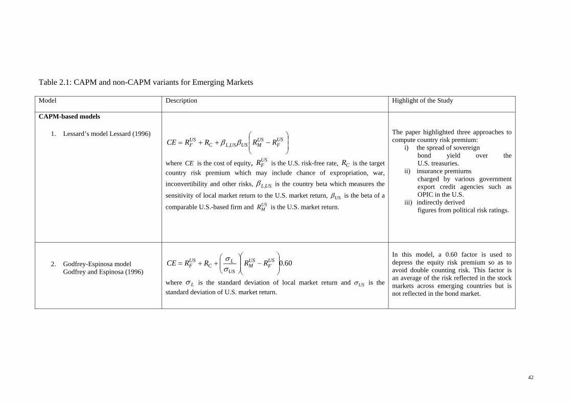
Table 2.1: CAPM and non-CAPM variants for Emerging Markets
Model Description Highlight of the Study
CAPM-based models
1. Lessard’s model Lessard (1996)
US
FUSMUSUSLC
USF RRRRCE ,
where CE is the cost of equity, USFR is the U.S. risk-free rate, CR is the target
country risk premium which may include chance of expropriation, war,
inconvertibility and other risks, USL, is the country beta which measures the
sensitivity of local market return to the U.S. market return, US is the beta of a
comparable U.S.-based firm and USMR is the U.S. market return.
The paper highlighted three approaches to compute country risk premium:
i) the spread of sovereign bond yield over the U.S. treasuries.
ii) insurance premiums charged by various government export credit agencies such as OPIC in the U.S.
iii) indirectly derived figures from political risk ratings.
2. Godfrey-Espinosa model Godfrey and Espinosa (1996)
60.0
US
FUSM
US
LC
USF RRRRCE
where L is the standard deviation of local market return and US is the
standard deviation of U.S. market return.
In this model, a 0.60 factor is used to depress the equity risk premium so as to avoid double counting risk. This factor is an average of the risk reflected in the stock markets across emerging countries but is not reflected in the bond market.

43
Table 2.1, continued.
3. Mariscal-Hargis model Mariscal and Hargis (1999)
RRRRRCE USF
USM
US
LLC
USF
1
where L measures the sensitivity of local firm returns to the local market
returns, R is the correlation between the local stock market and the bond market returns.
The inclusion of R1 to replace the
fixed adjustment of 0.60 can be thought of as a better adjustment for double counting risk.
4. Adjusted Local CAPM Pereiro (2001)
21 RRRRRCE LF
LMLC
LF
where LFR is the local risk-free rate and L
MR is the local market returns and 2R is the coefficient of determination of the regression between the volatility
of local market returns and the variation of country risk.
The inclusion of 21 R factor depresses
the equity risk premium to somewhat alleviate the problem of double-counting risk.
5. Adjusted Hybrid CAPM Pereiro (2001)
2, 1 RRRRRCE G
FGMGGGLC
GF
where GFR is the global risk-free rate, G
MR is the global market return, GL, is
the country beta which measures the sensitivity of local market return to the global market return and GG is the average unlevered beta of comparable
firms quoted in the global market.
The use of GG assumes cross-border
stability of betas. If this is a dubious assumption, a local beta may be used instead.

44
Table 2.1, continued.
6. Damodaran’s model Damodaran (2003)
US
FUSMLC
USF RRRRCE .
where is a measure of firm’s exposure to country risk.
The exposure factor, , is scaled around one where a of one indicates a firm with average exposure to country risk while a above or below one indicating above or below average exposure to country risk.
Non-CAPM-based models
7. Erb-Harvey-Viskanta model
Erb et al. (1996)
1,101, ln tiitti CCRCS
where CS is the semi-annual return in U.S. dollars for country i, CCR is the country credit rating, t is measured in half years and is the regression residual.
This model relates expected returns to credit rating where the “reward for risk” is measured by 1 .
8. Downside Risk model Estrada (2000; 2001)
US
FUSM
USF RRRMRCE
where RM is a risk measure.
The RM is a downside risk measure, taken as the ratio between the semi-standard deviation of returns with respect to the mean in the local market and the semi-standard deviation of returns with respect to the mean in the world market.

45
The aim of Lessard’s (1996) study was to help U.S. companies in the evaluation of their
offshore projects, especially those in emerging markets. According to Lessard (1996),
the cost of equity is given as the summation of a default risk-free rate and the risk
premium for market covariance risk. This risk premium, in turn, is defined as beta
(covariability of the project with the benchmark U.S. market portfolio) multiplied by the
risk premium on the benchmark market portfolio. Assuming that the relation between
the risk of a project with the local economy risk is same as that of a comparable project
in the home country, the project beta can then be estimated as the beta of the
comparable home country project multiplied by the country beta (the beta of the local
market portfolio relative to the home-market portfolio). The highlight of Lessard’s
(1996) study is the incorporation of a country risk premium4 in the risk-free rates where
the country risk premium can be computed using (i) the spread of sovereign bond yield
over the U.S. treasuries, (ii) insurance premiums charged by various government export
credit agencies, such as OPIC in the U.S. and EFIC in Australia to insure against
expropriation, war, etc. and (iii) country and political risk ratings published by
organizations like Euromoney and the Economist Intelligence Unit.
Nevertheless, one drawback of Lessard’s (1996) model is that it tends to overestimate
cost of equity. Godfrey and Espinosa (1996) argued that country risk may already be
present in the market risk premium and thus, including a country risk premium into the
risk-free rate will lead to double-counting. Analyzing returns from portfolios built based
on lagged country credit risk ratings for 40 national equity indices where 21 were for
developed markets and 19 for emerging markets, Erb et al. (1995) found that on average,
country risk explained about 40 percent of the cross-sectional variation in market return
variations. This means that the remaining 60 percent is explained by pure stock market
4 Several papers such as Herston and Rouwenhorst (1994) and Griffin and Karolyi (1998) documented that the effect of country risk on stock returns is often more sizeable than the sectoral effect.
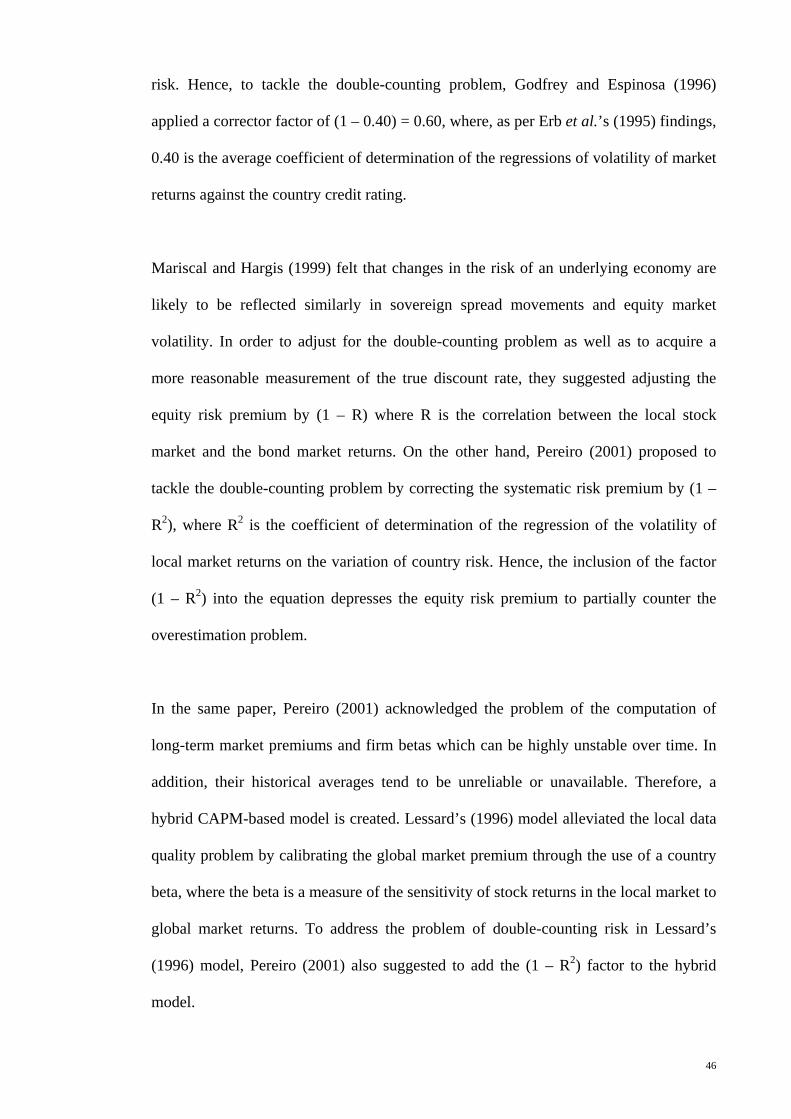
46
risk. Hence, to tackle the double-counting problem, Godfrey and Espinosa (1996)
applied a corrector factor of (1 – 0.40) = 0.60, where, as per Erb et al.’s (1995) findings,
0.40 is the average coefficient of determination of the regressions of volatility of market
returns against the country credit rating.
Mariscal and Hargis (1999) felt that changes in the risk of an underlying economy are
likely to be reflected similarly in sovereign spread movements and equity market
volatility. In order to adjust for the double-counting problem as well as to acquire a
more reasonable measurement of the true discount rate, they suggested adjusting the
equity risk premium by (1 – R) where R is the correlation between the local stock
market and the bond market returns. On the other hand, Pereiro (2001) proposed to
tackle the double-counting problem by correcting the systematic risk premium by (1 –
R2), where R2 is the coefficient of determination of the regression of the volatility of
local market returns on the variation of country risk. Hence, the inclusion of the factor
(1 – R2) into the equation depresses the equity risk premium to partially counter the
overestimation problem.
In the same paper, Pereiro (2001) acknowledged the problem of the computation of
long-term market premiums and firm betas which can be highly unstable over time. In
addition, their historical averages tend to be unreliable or unavailable. Therefore, a
hybrid CAPM-based model is created. Lessard’s (1996) model alleviated the local data
quality problem by calibrating the global market premium through the use of a country
beta, where the beta is a measure of the sensitivity of stock returns in the local market to
global market returns. To address the problem of double-counting risk in Lessard’s
(1996) model, Pereiro (2001) also suggested to add the (1 – R2) factor to the hybrid
model.
47
Damodaran (2003) believed firms in a market should have exposure to country risk that
differs from their exposure to other market risks. He introduced an exposure factor,
lambda, to measure a firm’s exposure to country risk. The lambda could be measured
using one of three variables. The first and simplest method is to measure lambda based
totally on where a firm generates its revenues. Using this method, the lambda is
obtained by dividing the percentage of revenues generated in the country for the firm of
interest by the average percentage for the firms in the country. The second method is
based upon the most recent accounting earnings and their variation over time.
Theoretically, a firm’s earnings that are more exposed to country risk should increase
(decrease) as country risk decreases (increases). The third measure is to use stock prices
to estimate firm risk exposure. This method is similar to the conventional beta estimates
except that stock returns were regressed against bond returns instead of the equity
market returns. While each of the three methods has its own drawback, the key to
measure exposure to country risk should be based on where a firm operates and not
where it is incorporated.
The existence of empirical evidence, for example, Harvey (1995) who found betas of
emerging markets to be largely uncorrelated to variation in expected returns in a single-
factor model framework, has motivated the development of non-CAPM-based models.
In fact, in developing their model, Erb et al. (1996) also found no significant relation
between beta and expected returns when using a broader cross-sectional sample of
countries than that used by Harvey (1995). An alternative solution provided by Bekaert
and Harvey (1995) is to use a time-varying approach where the cost of equity is allowed
to change over time. However, the method is criticized for its complexity in the
estimation procedure which makes it unattractive to practitioners who typically seek
48
more straightforward methods (Estrada, 2000; Chen and Chen, 2004; Collins and
Abrahamson, 2006).
The model of Erb et al. (1996) is categorized as “non-CAPM-based” asset pricing
model as it does not use the standard beta or market risk premium to arrive at a discount
rate. The model uses Institutional Investors’ country credit ratings to establish forward-
looking rates that represent expected returns on investments of average risk within each
country. A regression was estimated by combining all market returns for 47 countries
and credit ratings into one large model. A log-linear model was used following the
argument that as credit rating falls to a low level, expected returns may increase faster
than predicted by a linear model. The slope coefficient was found to be significantly
negative, suggesting that higher credit ratings are associated with lower average returns.
Nevertheless, the model of Erb et al. (1996) can only be applied for estimating cost of
equity at a country-wide level but not at the firm-level.
Estrada (2000) commented that beta values seem to be too small to accommodate the
figures for the cost of equity that most investors deem as reasonable, implying that beta
does not accurately measure risk in emerging markets. If beta is maintained as a
measure of risk, many emerging markets would have low investment risks. Recognizing
the problem of beta especially when applied to emerging markets, Estrada (2000)
proposed the downside risk measure, that is, semi-deviation or semi-variance, which he
felt can perform better than beta in capturing expected returns of emerging markets. He
argued that the downside risk models are preferable since they produce estimates of cost
of equity that are halfway between the ‘rather low’ figures produced by the systematic
risk (beta) approach and the higher figures generated by the total risk method.
49
Besides providing more reasonable cost of equity estimates for emerging markets, the
downside risk method has several attractive features (Estrada, 2000). Among the
features are easy implementation of the method, ability to be applied to both market
level and firm level analysis, it is not based on subjective measures of risk, it can be
adjusted to any desired benchmark return and most importantly, downside risk captures
the portion of risk that investors want to avoid. Further support for downside risk
measure is provided by Harvey (2000) who documented that semi-deviation explains a
substantial part of the variations in the stock returns of emerging markets. Estrada (2001)
extended his test across industries in emerging markets and the results supported the
semi-deviation as an appropriate measure of risk in emerging markets.
Downside risk, also referred to as lower partial moments, was first introduced by Roy
(1952). He believed investors will prefer safety of principal first and will set some
minimum acceptable return that will preserve the principal. Roy’s concept became
influential in the development of downside risk measures. Earlier studies such as those
of Hogan and Warren (1974), Bawa and Lindenberg (1977) and Harlow and Rao (1989)
have also proposed CAPM-like models based on downside risks. In their paper, Hogan
and Warren (1974) suggested that given the strong support found for semi-variance
(downside risk) as a more appropriate risk measure than variance, a CAPM based on
semi-variance might provide superior explanation on capital market behaviour.
However, compared to the standard risk measure, beta, downside risk has been tested
less extensively.
Recent research interest attempted to compare the performance of standard risk measure
to downside risk measure. In a sample of 27 emerging markets, Estrada (2002, 2007)
documented evidence that about one third of the emerging markets showed a difference
50
in required returns generated by beta and downside beta that is larger than 300 basis
points a year, a differential that is simply too large for practitioners to ignore. Chen and
Chen (2004) also found the downside risk to have a strong explanatory power on stock
returns. Nevertheless, using equity data from the U.K., Pedersen and Hwang (2007)
found although downside beta explained stock returns better than the traditional CAPM,
the proportion of equities benefitting from using the former is not large enough to
improve asset pricing models significantly.
In sum, asset pricing models modified specifically for use in emerging markets are
relatively new in view that most of them have only being introduced in the 1990s or
after the new millennium. These models have yet to be studied or used extensively in
the literature. Much work needs to be done in order to establish the strength of these
models so that investors are more confident in using them to obtain cost of equity
estimates.
2.4 Measuring Cost of Equity on a Sectoral Basis
An early paper by Lessard (1974) documented that a sectoral factor significantly
explains the proportion of individual stock returns that were unexplained by a world
market factor. An important implication from his results is that the sectoral factor plays
a significant role in explaining the variation of market returns. Based on equity price
indices for 24 countries including Malaysia, Roll (1992) reported that the sectoral factor
is more important than the exchange rate in explaining stock price behaviour for most
countries. The argument is that different sectors have differing impacts on the stock
exchange, for example, mining is important for producer countries like South Africa but
relatively unimportant for raw material importer countries like Hong Kong. Therefore,
51
countries with similar sectors tend to have similar market behaviour than countries with
different sectors.
Bekaert and Harvey (1995) noted that returns of a market may be weakly or negatively
correlated to the world market returns even though the market could be perfectly
integrated into the world market, due to its sectoral mix that is grossly different from the
average world mix. Hardouvelis et al. (2007) examined the behaviour of industrial
sectors across the Economic and Monetary Union (EMU) countries. They believe that
there is no reason to assume all sectors in a country will benefit from higher stock
market integration just because the country does. The issue of whether the EMU led to a
convergence in cost of equity within a sector across the member countries or across
different sectors within a given country has important investment implications with
regards to whether asset allocation should be optimized across countries or across
sectors. Their study revealed strong convergence in the cost of equity across the EMU
countries within a given industrial sector, but little convergence across the different
sectors of a given country. The implication for portfolio managers is that sectoral effects
are becoming more important.
Realizing the increasing importance of the sectoral factor, Collins and Abrahamson
(2006) examined the cost of equity in a sample of African equity markets on a sectoral
basis. Using the FTSE Global Classification System, they measured cost of equity for
ten sectors, namely, Financials, Resources, Basic Industries, Non-Cyclical Goods,
Cyclical Services, General Industrials, Clyclical Goods, Non-Cyclical Services, Utilities,
and Information Technology, across six African markets (Egypt, Kenya, Morocco,
Namibia, South Africa, and Zimbabwe), covering the time period of 1999-2002.
Concurring with the findings of Estrada (2000) who emphasized the importance of

52
downside risk measures for emerging markets, Collins and Abrahamson (2006) took
averages from four cost of equity measures based on standard deviation, beta, semi-
deviation with respect to mean and downside beta. They found that Non-Cyclical Goods,
Financials and Basic Industries had the lowest cost of equity estimates while Resources,
Utilities, Non-Cyclical Services and Information Technology were the sectors with the
highest cost of equity estimates.
In a recent study, Hearn and Piesse (2009) found considerable dispersion of cost of
equity between various industrial sectors in a sample consisting of eight African
markets (Morocco, Tunisia, Egypt, Kenya, Nigeria, Zambia, Botswana and South
Africa). For all countries, the Financial sector recorded the highest cost of equity while
lowest cost of equity was found for blue chip stocks in Tunisia, Morocco, Namibia and
South Africa. For the individual countries, the dispersion of cost of equity in the
Moroccan market ranges from 15.43 percent and 17.26 percent for the industrial and
diversified sectors to 25.37 percent for the consumer-cyclical sector, while the Tunisian
market exhibited the greatest dispersion between sectors with values that ranged from
1.70 percent for the consumer non-cyclical sector to 11.19 percent for the finance sector.
The implication of these studies is that although equity markets may have converged
following the globalization waves, there could be little convergence across industries
within a market itself. The wide dispersion in cost of equity estimates that is still
observed warrants an analysis to be done on a sectoral basis.
2.5 The Determinants of Cost of Equity
Given the importance of cost of equity for making financial decisions and the amount of
work that has been dedicated to find appropriate asset pricing models for its estimation,
53
the subsequent quest will be to determine the factors that affect cost of equity. As there
could be many factors that might influent cost of equity, the scope of this review is
narrowed to prominent issues or events in the 1990s that have triggered research on the
effect of these phenomena on cost of equity. This section is also dedicated to review the
influence of the fundamentals, specifically the firm-related accounting variables and
market-related variables on cost of equity.
The outbreak of international diversifications and cross-listing activities in the 1990s
led to research interest in exploring the effect of these activities on cost of equity (see
for example, Foerster and Karolyi, 1993,1999; Karolyi, 1998; Doukas and Switzer,
2000; Singh and Nejadmalayeri, 2004). The extensive survey of studies on cross-
listings provided by Karolyi (1998), for instance, concluded that the effect of listing
decisions can result in a net reduction of approximately 126 basis points in cost of
equity. This is due to a significant decrease in domestic market risk while only a slight
increase in global market risk and foreign exchange risk. Higher degree of international
diversification also resulted in lower cost of capital as evident in the study of Singh and
Nejadmalayeri (2004). Using a sample of 90 French firms from 1996 to 1999, the effect
is observable even after controlling for other variables such as debt, equity risk, firm
size and asset structure.
Another closely related area to international diversifications and cross-listings is the
effect of capital market liberalization on cost of equity. The intuition is that in a
segmented capital market, cost of equity is related to variability in the local market
returns. On the other hand, in an integrated capital market, cost of equity is related to
covariance with the world market returns. Since local market returns are normally more
volatile, as capital markets open up or liberalize and the covariance with the world
54
capital market increases, their cost of equity should decrease. A number of studies
documented evidence that capital market liberalization reduces cost of equity (see for
example, Bekaert and Harvey, 2000; Henry, 2000; Chari and Henry 2004). Taking a
step further, Ameer (2007) tested the effect of stock market liberalization at the firm-
level and found that there was significant difference in the decline of cost of equity
among firms once firm heterogeneous characteristics were taken into account. In a
recent study, Li (2010), using sector-level data for 19 emerging markets and 18
developed countries from 1980 to 2000, provided evidence that sectors that were highly
dependent on external funding seemed to grow faster after liberalization. This supports
the hypothesis that capital market liberalization results in lower cost of equity.
A series of financial scandal outbreaks in the 1990s might have motivated studies on the
effect of legal institutions and securities regulation (Daouk et al., 2006; Hail and Leuz,
2006), as well as disclosures and corporate governance (Botosan, 1997; Bhattacharya
and Daouk, 2002; Eaton et al., 2007; Chen et al., 2009; Guedhami and Mishra, 2009)
on cost of equity. It was argued that a well-functioning legal system reduces monitoring
and enforcement costs to investors, which may result in investors demanding a lower
return on their capital. Testing on a sample consisting of 35,118 firm-year observations
from 40 countries spanning from 1992 to 2001, Hail and Leuz (2006) found that firms
in countries with effective legal institutions had lower cost of equity than they do in
countries with weak legal systems. Based on four different models of implied cost of
equity used by Hail and Leuz (2006), Guedhami and Mishra (2009) reported that excess
control negatively affects firm value, and this is reflected in the firm’s discount rate. In
addition, consistent with the findings of Hail and Leuz (2006), they found that legal
institutions have significant influence on cost of equity too.
55
The discussion so far involves studies on events related to international investment,
capital market liberalization and financial scandals. On the other hand, there are also
studies which focus on the fundamentals, especially financial statements of firms. Data
from financial statements were found to be value-relevant to public listed firms (see for
example, Barth et al. 2001; Kothari, 2001). The importance of financial statement
increases as a firm matures and its financial position become increasingly associated
with its equity value (Hand, 2005). Nevertheless, in most studies, exploring financial
statement data as potential determinants of cost of equity is not the core objective, but a
peripheral product of the analysis on the impact of other factors such as legal
institutions and securities regulation (Hail and Leuz, 2006), financial liberalization
(Ameer, 2007), and corporate governance (Chen et al., 2009, Guedhami and Mishra,
2009) on cost of equity.
A summary of studies on the relationship between various variables and cost of equity
is provided in Table 2.2. The table is divided into two parts. The first part summarizes
studies with emphasis on accounting-based variables and (or) market-based variables.
The accounting-based variables are those measured using accounting information only
while the market-based variables are constructed from the relation between accounting
data and market data. Part two of Table 2.2 includes studies that focus on other
variables such as international diversification and corporate governance but also
includes accounting-based variables or market-based variables in the study.
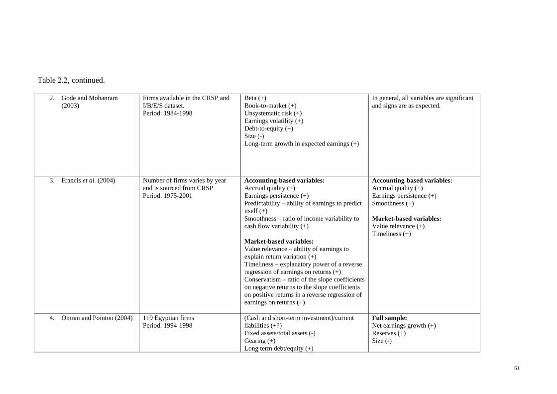
Gebhardt et al. (2001) and Gode and Monhanram (2003) indirectly explored the
determinants for cost of equity through implied risk premium. Gebhardt et al. (2001)
examined the relationship of implied risk premium with various risk categories which
can be grouped into market volatility, leverage, liquidity and information environment,
56
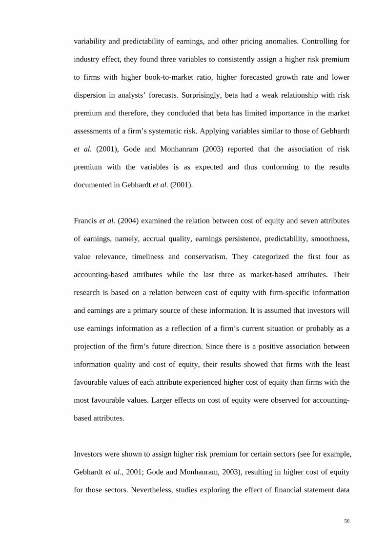
variability and predictability of earnings, and other pricing anomalies. Controlling for
industry effect, they found three variables to consistently assign a higher risk premium
to firms with higher book-to-market ratio, higher forecasted growth rate and lower
dispersion in analysts’ forecasts. Surprisingly, beta had a weak relationship with risk
premium and therefore, they concluded that beta has limited importance in the market
assessments of a firm’s systematic risk. Applying variables similar to those of Gebhardt
et al. (2001), Gode and Monhanram (2003) reported that the association of risk
premium with the variables is as expected and thus conforming to the results
documented in Gebhardt et al. (2001).
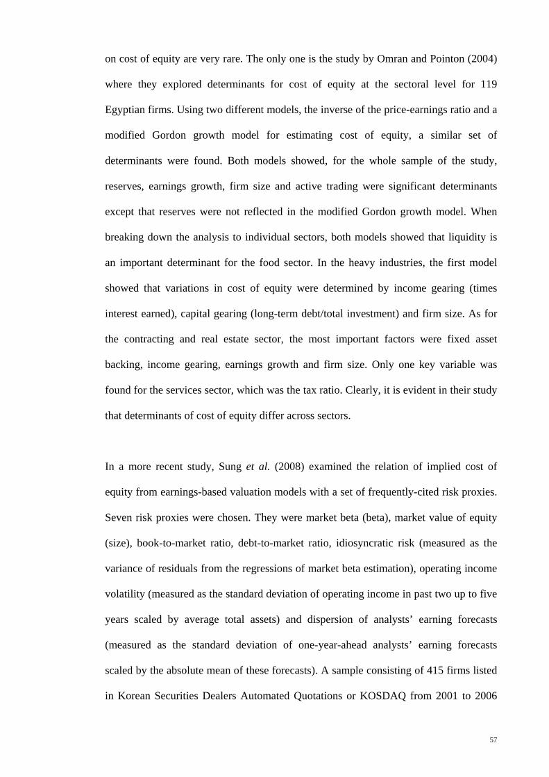
Francis et al. (2004) examined the relation between cost of equity and seven attributes
of earnings, namely, accrual quality, earnings persistence, predictability, smoothness,
value relevance, timeliness and conservatism. They categorized the first four as
accounting-based attributes while the last three as market-based attributes. Their
research is based on a relation between cost of equity with firm-specific information
and earnings are a primary source of these information. It is assumed that investors will
use earnings information as a reflection of a firm’s current situation or probably as a
projection of the firm’s future direction. Since there is a positive association between
information quality and cost of equity, their results showed that firms with the least
favourable values of each attribute experienced higher cost of equity than firms with the
most favourable values. Larger effects on cost of equity were observed for accounting-
based attributes.
Investors were shown to assign higher risk premium for certain sectors (see for example,
Gebhardt et al., 2001; Gode and Monhanram, 2003), resulting in higher cost of equity
for those sectors. Nevertheless, studies exploring the effect of financial statement data
57
on cost of equity are very rare. The only one is the study by Omran and Pointon (2004)
where they explored determinants for cost of equity at the sectoral level for 119
Egyptian firms. Using two different models, the inverse of the price-earnings ratio and a
modified Gordon growth model for estimating cost of equity, a similar set of
determinants were found. Both models showed, for the whole sample of the study,
reserves, earnings growth, firm size and active trading were significant determinants
except that reserves were not reflected in the modified Gordon growth model. When
breaking down the analysis to individual sectors, both models showed that liquidity is
an important determinant for the food sector. In the heavy industries, the first model
showed that variations in cost of equity were determined by income gearing (times
interest earned), capital gearing (long-term debt/total investment) and firm size. As for
the contracting and real estate sector, the most important factors were fixed asset
backing, income gearing, earnings growth and firm size. Only one key variable was
found for the services sector, which was the tax ratio. Clearly, it is evident in their study
that determinants of cost of equity differ across sectors.
In a more recent study, Sung et al. (2008) examined the relation of implied cost of
equity from earnings-based valuation models with a set of frequently-cited risk proxies.
Seven risk proxies were chosen. They were market beta (beta), market value of equity
(size), book-to-market ratio, debt-to-market ratio, idiosyncratic risk (measured as the
variance of residuals from the regressions of market beta estimation), operating income
volatility (measured as the standard deviation of operating income in past two up to five
years scaled by average total assets) and dispersion of analysts’ earning forecasts
(measured as the standard deviation of one-year-ahead analysts’ earning forecasts
scaled by the absolute mean of these forecasts). A sample consisting of 415 firms listed
in Korean Securities Dealers Automated Quotations or KOSDAQ from 2001 to 2006
58
was used in the study. They found that the average implied cost of equity was positively
associated with beta, debt-to-market ratio and operating income volatility, while
negatively related to size.
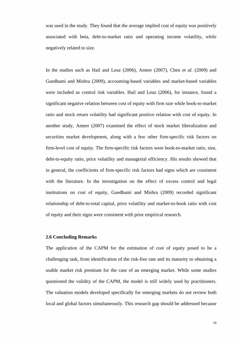
In the studies such as Hail and Leuz (2006), Ameer (2007), Chen et al. (2009) and
Guedhami and Mishra (2009), accounting-based variables and market-based variables
were included as control risk variables. Hail and Leuz (2006), for instance, found a
significant negative relation between cost of equity with firm size while book-to-market
ratio and stock return volatility had significant positive relation with cost of equity. In
another study, Ameer (2007) examined the effect of stock market liberalization and
securities market development, along with a few other firm-specific risk factors on
firm-level cost of equity. The firm-specific risk factors were book-to-market ratio, size,
debt-to-equity ratio, price volatility and managerial efficiency. His results showed that
in general, the coefficients of firm-specific risk factors had signs which are consistent
with the literature. In the investigation on the effect of excess control and legal
institutions on cost of equity, Guedhami and Mishra (2009) recorded significant
relationship of debt-to-total capital, price volatility and market-to-book ratio with cost
of equity and their signs were consistent with prior empirical research.
2.6 Concluding Remarks
The application of the CAPM for the estimation of cost of equity posed to be a
challenging task, from identification of the risk-free rate and its maturity to obtaining a
usable market risk premium for the case of an emerging market. While some studies
questioned the validity of the CAPM, the model is still widely used by practitioners.
The valuation models developed specifically for emerging markets do not review both
local and global factors simultaneously. This research gap should be addressed because

59
if an emerging market is partially integrated to the world capital market, then a model
which considers both local and global factors might offer better explanatory power on
firm stock returns. Hence, better cost of equity estimates could be obtained. Likewise,
systematic risks alone may not be sufficient for the estimation of cost of equity. The
increasingly relevance of downside risk must be taken into consideration in the
estimation of cost of equity for emerging markets. There is also clearly a lack of studies
on cost of equity determinants, in particular, on a sectoral basis. Efforts to find such
determinants will only be meaningful following the establishment of appropriate
measures of cost of equity.

60
Table 2.2: Association of Various Explanatory Variables with Cost of Equity
Study Sample Variables Used in Analysis (Expected Sign) Significant Variables in Results (Sign)
Accounting/Market-Related variables as primary focus
1. Gebhardt et al. (2001)
All U.S. firms from the NYSE and AMEX obtained from the CRSP and available on I/B/E/S dataset. Number of firms varies by year. Period: 1979-1995
Market volatility: Beta (+) Standard deviation of stock returns (+) Leverage: Debt-to-book value of equity (+) Debt-to-market value of equity (+) Liquidity and information environment: Size (-) Analyst coverage (-) Average dollar trading volume (-) Variability and predictability of earnings:Mean absolute errors of forecast (+/-) Earnings variability (+/-) Dispersion in analysts’ forecasts (+/-) Market anomaly variables: Long-term growth in earnings (-) Book-to-market (+) Price momentum (+) Turnover (-)
Book-to-market (+) Dispersion in analysts’ forecasts (-) Long-term growth in earnings (+)
61
Table 2.2, continued.
2. Gode and Mohanram (2003)
Firms available in the CRSP and I/B/E/S dataset. Period: 1984-1998
Beta (+) Book-to-market (+) Unsystematic risk (+) Earnings volatility (+) Debt-to-equity (+) Size (-) Long-term growth in expected earnings (+)
In general, all variables are significant and signs are as expected.
3. Francis et al. (2004) Number of firms varies by year and is sourced from CRSP Period: 1975-2001
Accounting-based variables: Accrual quality (+) Earnings persistence (+) Predictability – ability of earnings to predict itself (+) Smoothness – ratio of income variability to cash flow variability (+) Market-based variables: Value relevance – ability of earnings to explain return variation (+) Timeliness – explanatory power of a reverse regression of earnings on returns (+) Conservatism – ratio of the slope coefficients on negative returns to the slope coefficients on positive returns in a reverse regression of earnings on returns (+)
Accounting-based variables: Accrual quality (+) Earnings persistence (+) Smoothness (+) Market-based variables: Value relevance (+) Timeliness (+)
4. Omran and Pointon (2004)
119 Egyptian firms Period: 1994-1998
(Cash and short-term investment)/current liabilities (+?) Fixed assets/total assets (-) Gearing (+) Long term debt/equity (+)
Full sample: Net earnings growth (+) Reserves (+) Size (-)

62
Table 2.2, continued.
Long term debt/total investment (+) Net earnings growth (+) Net fixed asset growth (+) Q-ratio (+) Quick ratio (+?) Reserves (-) Size (-) Standard deviation of earnings (+) Tax/net profit before tax (-) Times interest earned (-)
Food sector: (Cash and short-term investments)/Current liabilities (-) Quick ratio (+) Standard deviation of earnings (+) Times interest earned (+) Heavy industry: Long term debt/total investment (+) Size (-) Times interest earned (-) Contracting and Real Estates: Fixed asset/total assets (+) Net earnings growth (+) Net fixed asset growth (+) Size (-) Standard deviation of earnings (+) Times interest earned (-) Services: Tax/net profit before tax (+)
5. Sung et al. (2008) 415 firms listed on KSE/KOSDAQ. Period: 2001-2006
Beta (+) Book-to-market (+) Debt-to-market (+) Dispersion of analysts’ earnings forecasts (+) Idiosyncratic risk (+) Operating income volatility (+) Size (-)
Beta (+) Debt-to-market (+) Operating income volatility (+) Size (-)

63
Table 2.2, continued.
Accounting/Market-Related variables as control risk factors
6. Hail and Leuz (2006)
35,l22 firm-year observations from 40 countries contained in Worldscope. Period: 1992-2001
Beta (+) Book-to-market (+) FBIAS – one-year-ahead analyst forecast error (+) Inflation (+) MVAR – component of four proxies for macroeconomic variability (+) Size (-) Stock return volatility (+)
All are significant and have predicted sign.
7. Ameer (2007) Listed non-financial firms, number in bracket indicates number of firms [India (50); Indonesia (35); Malaysia (50); Pakistan (20); South Korea (50); Thailand (37)] Period: 1990-2004
Asset turnover ratio (+) Book-to-market (+) Debt-to-equity (+) Size (-) Price volatility (+)
Debt-to-equity (+) Asset turnover ratio (+)
8. Chen et al. (2009) Firms covered in Credit Lyonnais Securities Asia (CLSA) Emerging Markets published in 2001 and 2002.
Analysts’ forecast errors (-) Beta (+) Book-to-market (+) Liquidity (-) Ownership concentration (-) Price momentum (-)
All are significant and have predicted sign except for Liquidity.
9. Guedhami and Mishra (2009)
1207 firms from 9 Asian and 13 Western European countries. Period: 1996-1999
Analyst coverage (-) Debt-to- total capital (+) Dispersion of analyst forecasts (+) Excess control (+) Legal institutions variables (-) Long-term growth rate (+) Market-to-book (-) Price volatility (+)
All are significant and have predicted sign.

64