Chapter 2 - Linear Equations

2.1 Solving Linear Equations

One of the most common problems in scientificcomputing is the solution of linear equations.

It is a problem in its own right, but it also occurs as asub-problem for many other problems.

For example, as we will see, the solution of a nonlinearsystem of equations is typically approximated througha sequence of solutions of linear systems.

The discretization of a linear elliptic partial differentialequation typically leads to the solution of a (highlystructured) linear system of equations.

1

Here is a simple example: Three unknowns x, y, and zsatisfy

2x + 4y − 2z = 2,4x + 9y − 3z = 8,−2x − 3y + 7z = 10.

The goal is to find the magical values of x, y, z thatsatisfy all 3 of the above equations.

Before we talk about strategies to solve linear systems,we start by standardizing the notation to generalizethe problem to m equations in m unknowns.

Relabel the unknowns x = (x1, x2, . . . , xm)T ,the coefficients a11, a21, . . . , am1, a21, a22, . . . , a2m,. . . , am1, am2, . . . , amm, and the right-hand side valuesb = (b1, b2, . . . , bm)T .

2

a11x1 + a21x2 + . . .+ a1mxm = b1,

a21x1 + a22x2 + . . .+ a2mxm = b2,

...

am1x1 + am2x2 + . . .+ ammxm = bm.

In matrix notation:

Ax = b.

Formally, the solution to this problem is

x = A−1b.

However, in practice we never actually find the inverseof A and then multiply it by b to get x!

3

Suppose we wish to solve the easy equation 7x1 = 21.

If we find the inverse of 7 and multiply it by 21 to getx1, this requires 2 floating-point operations and suffersfrom roundoff error:

x1 = 7−1 × 21 ≈ 0.142857× 21 ≈ 2.99997.

The cheapest and most accurate way to solve thisequation is by division:

x1 =21

7= 3.

Although this example may look artificial, theseprinciples extend to larger systems, where they becomeeven more important!

4

2.2 The \ Operator

To emphasize the distinction between solving linearequations and computing inverses, Matlab uses thebackward slash (or backslash) operator \.

If A is a matrix of any size and shape and b is avector with as many rows as A, then the solution tothe system of simultaneous equations Ax = b can becomputed in Matlab by x = A\b.

If it helps, you can think of this as “left-dividing” bothsides of the equation by the coefficient matrix A.

→ Because matrix multiplication is not commutativeand A occurs on the left in the original equation, thisis left division.

Note 1. This operator can be applied even if A isnot square; i.e., the number of equations is not thesame as the number of unknowns.

However, in this course, we always assume A is square.

5

Note 2. Solving the linear system Ax = b formultiple right-hand sides b1, b2, . . . , bp, can bedone all at once by defining B = [b1,b2, . . . ,bp] andusing the command X = A\B.

The answers come out in matrix X = [x1,x2, . . . ,xp].

6

2.3 Simple Examples

The simplest kinds of linear systems to solve are oneswhere the unknowns are decoupled. For example,

0.3x1 = 3, 5x2 = 1.5, 2x3 = −4.

In matrix form,0.3 0 00 5 00 0 2

x1x2x3

=

31.5−4

.Note that the coefficient matrix is diagonal.

In this case, the unknowns can be solved forindependently ; e.g., in any order, or in batches ifyou have a parallel computer.

7

It is possible to reduce a non-singular matrix to diagonalform and then solve for the unknowns; this is knownas Gauss–Jordan elimination.

In practice, Gauss–Jordan elimination is more expensivethan another method (Gaussian elimination) that worksjust as well.

Gaussian elimination is based on a systematic1

procedure to reduce the coefficient matrix A to upper-triangular form.

What’s the advantage of upper-triangular form?

It turns out that you can solve for the unknowns in anupper-triangular system of linear equations one afterthe other.

We will see this in the next section; but for futurereference and to appreciate the concept of equationmanipulation as matrix multiplication, we first look atpermutation and triangular matrices.

1So that it can be programmed!

8

2.4.1 Permutation Matrices

Sometimes you may want to interchange rows orcolumns of a matrix. This operation can be representedby matrix multiplication by a permutation matrix .

Definition 1. A permutation matrix P is a matrixmade by taking the identity matrix and interchangingits rows or columns.

In other words, P has exactly one 1 in each row andcolumn; all the other elements are 0.

Here is an example of a permutation matrix:

P =

0 0 0 11 0 0 00 0 1 00 1 0 0

.How is it related to the 4× 4 identity matrix I?

Row 4 of I is Row 1 of P; Row 1 of I is Row 2 of P;Row 3 of I is Row 3 of P; Row 2 of I is Row 4 of P.

9

=⇒ The matrix PA has A’s Row 4 as its Row 1,A’s Row 1 as its Row 2, A’s Row 3 as its Row 3, andA’s Row 2 as its Row 4.

Similarly,

Col 2 of I is Col 1 of P; Col 4 of I is Col 2 of P;Col 3 of I is Col 3 of P; Col 1 of I is Col 4 of P.

=⇒ The matrix APT has A’s Col 4 as its Col 1, A’sCol 1 as its Col 2, A’s Col 3 as its Col 3, and A’s Col2 as its Col 4.

Note 3. A compact way to store P (or simply keeptrack of permutations) is in a vector.

e.g., The row interchanges represented by P in ourexample can be stored as the vector p = [4 1 3 2].

A quick way to create a matrix B from interchangingthe rows and columns of A via p is B = A(p,p).

Permutation matrices are orthogonal matrices; i.e.,they satisfy

PTP = I, or equivalently P−1 = PT .

10

2.4.2 Triangular Matrices

An upper-triangular matrix has all its nonzero elementson or above the main diagonal.

A lower-triangular matrix has all its nonzero elementson or below the main diagonal.

A unit lower-triangular matrix is a lower-triangularmatrix with ones on the main diagonal.

Here are examples of an upper-triangular matrix U anda unit lower-triangular matrix L:

U =

1 2 30 4 50 0 6

, L =

1 0 02 1 03 4 1

.

11

Linear equations involving triangular matrices are easyto solve.

We focus on the case for upper-triangular systemsbecause it will be relevant in LU factorization.

One way to solve an m ×m upper-triangular system,Ux = b is to begin by solving the last equation forthe last variable, then the next-to-last equation forthe next-to-last variable, and so on, using the newlycomputed values of the solution along the way.

Here is some Matlab code to do this:

x = zeros(m,1);

for k = m:-1:1,

j = k+1:m;

x(k) = (b(k) - U(k,j)*x(j))/U(k,k);

end

12

2.4.3 Banded Matrices

A matrix A is called a banded matrix with lowerbandwidth p and upper bandwidth q if

ai,j = 0 if i > j + p or j > i+ q.

The band width of A is naturally defined as p+ q+1.

A has p sub-diagonals and q super-diagonals, and theband width is the total number of diagonals.

Important special cases of banded matrices are

• diagonal matrices (p = q = 0),tridiagonal matrices (p = q = 1),pentadiagonal matrices (p = q = 2),

...full matrices (p = q = bm/2c)

• bidiagonal matrices(lower: (p, q) = (1, 0), upper: (p, q) = (0, 1))

Hessenberg matrices (lower: q = 1; upper: p = 1)

13

2.5 LU Factorization

The LU factorization is the factorization of a matrixA into the product of a unit lower-triangular matrixand an upper-triangular matrix; i.e., A = LU.

The LU factorization is an interpretation of Gaussianelimination, one of the oldest numerical methods,generally named after Gauss.

It is perhaps the simplest systematic way to solvesystems of linear equations by hand, and it is also thestandard method for solving them on a computer.

Research between 1955 to 1965 revealed theimportance of two aspects of Gaussian eliminationthat were not emphasized in earlier work: the searchfor pivots and the proper interpretation of the effect ofrounding errors.

Pivoting is essential to the stability of Gaussianelimination!

14

The first important concept is that the familiar processof eliminating elements below the diagonal in Gaussianelimination can be viewed as matrix multiplication.

The elimination is accomplished by subtractingmultiples of each row from subsequent rows.

Before we see the details, let’s pretend we know howto do this in a systematic fashion.

The elimination process is equivalent to multiplying Aby a sequence of lower-triangular matrices Lk on theleft

Lm−1Lm−2 . . .L1A = U,

where Lk eliminates the elements below the diagonalin row k.

In other words, we keep eliminating elements belowthe diagonal until A has been reduced to an upper-triangular matrix, which we call U.

15

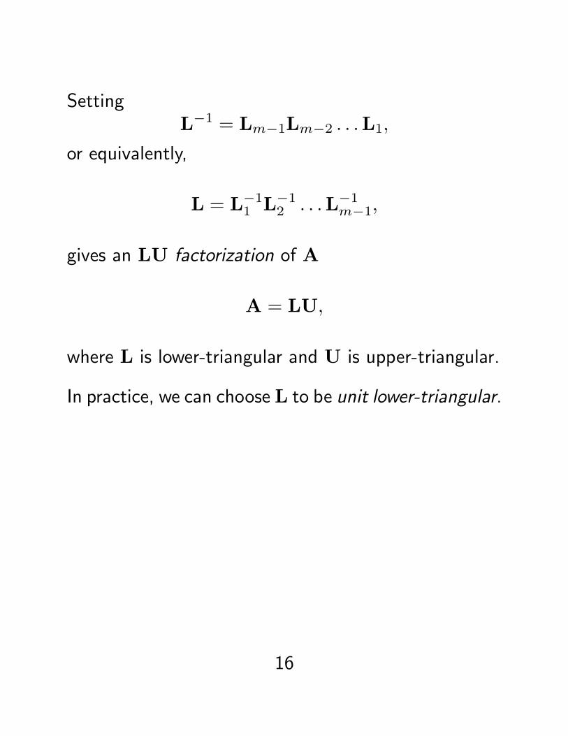
SettingL−1 = Lm−1Lm−2 . . .L1,

or equivalently,

L = L−11 L−12 . . .L−1m−1,

gives an LU factorization of A

A = LU,

where L is lower-triangular and U is upper-triangular.

In practice, we can choose L to be unit lower-triangular.

16

Example: Suppose A is 4× 4:× × × ×× × × ×× × × ×× × × ×

−→L1

× × × ×0 ∗ ∗ ∗0 ∗ ∗ ∗0 ∗ ∗ ∗

A L1A

× × × ×× × ×× × ×× × ×

−→L2

× × × ×× × ×0 ∗ ∗0 ∗ ∗

L1A L2L1A

× × × ×× × ×× ×× ×

−→L3

× × × ×× × ×× ×0 ∗

L2L1A L3L2L1A

3 EXAMPLE

Let

A =

2 1 1 04 3 3 18 7 9 56 7 9 8

.

(This particular A was chosen because it has a niceLU decomposition.)

17

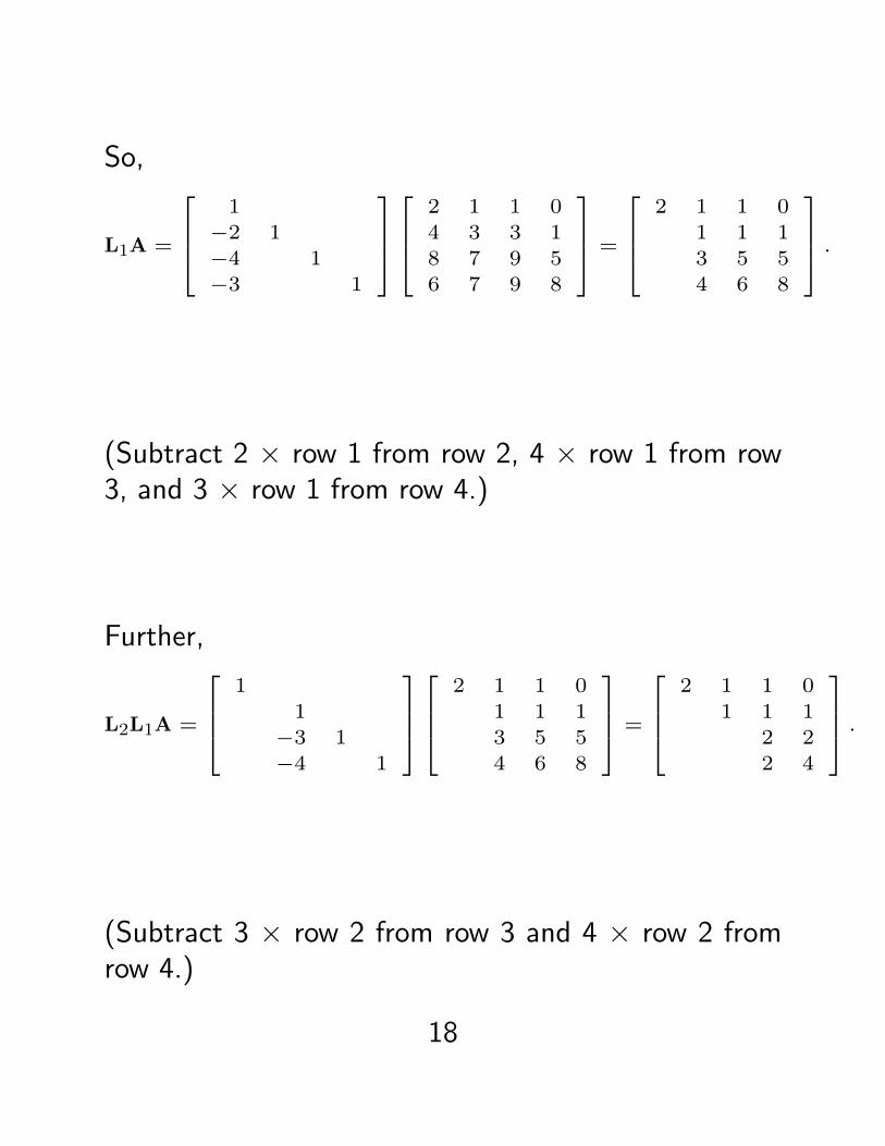
So,

L1A =

1−2 1−4 1−3 1

2 1 1 04 3 3 18 7 9 56 7 9 8

=

2 1 1 0

1 1 13 5 54 6 8

.

(Subtract 2 × row 1 from row 2, 4 × row 1 from row3, and 3 × row 1 from row 4.)

Further,

L2L1A =

1

1−3 1−4 1

2 1 1 01 1 13 5 54 6 8

=

2 1 1 0

1 1 12 22 4

.

(Subtract 3 × row 2 from row 3 and 4 × row 2 fromrow 4.)

18

Finally,

L3L2L1A =

1

11−1 1

2 1 1 01 1 1

2 22 4

=

2 1 1 0

1 1 12 2

2

= U.

(Subtract row 3 from row 4.)

To obtain A = LU, we need to form

L = L−11 L−12 L−13 .

This turns out to be easy, thanks to two happysurprises.

L−11 can be obtained from L1 by negating the off-diagonal entries:

L−11 =

1−2 1−4 1−3 1

−1

=

12 14 13 1

.

19

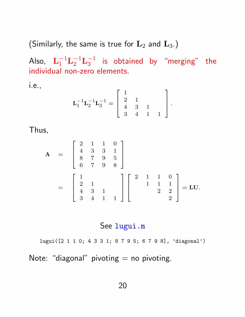
(Similarly, the same is true for L2 and L3.)

Also, L−11 L−12 L−13 is obtained by “merging” theindividual non-zero elements.

i.e.,

L−11 L

−12 L

−13 =

12 14 3 13 4 1 1

.

Thus,

A =

2 1 1 04 3 3 18 7 9 56 7 9 8

=

12 14 3 13 4 1 1

2 1 1 01 1 1

2 22

= LU.

See lugui.m

lugui([2 1 1 0; 4 3 3 1; 8 7 9 5; 6 7 9 8], ’diagonal’)

Note: “diagonal” pivoting = no pivoting.

20

To formalize the facts that we need (without proof!):

1. In Gaussian elimination, elimination of elementsbelow the diagonal in row k by row operationsagainst row k (the pivot row) can be viewed asleft-multiplication by a unit lower-triangular matrixwith elements ljk in column k with ljk = −(elementto eliminate)/(pivot).

2. Lk can be inverted by negating the off-diagonalelements −ljk (so L contains ljk),

3. L can be formed by merging the entries ljk.

Of course, in practice, the matrices Lk are never formedand multiplied explicitly.→ Only the quantities ljk are computed and stored,often in the lower triangle of A, which would otherwisecontain zeros upon reduction to U.

21

How does this help us solve Ax = b?

Writing this as LUx = b, this can now be solved bysolving two triangular systems.

First solve Ly = b for an intermediate variable y(forward substitution).

Then solve Ux = y for the unknown variable x (backsubstitution).

Once we have L and U, solving for the unknown x isquick and easy for any number of right-hand sides b.

22

Pivoting

Pure Gaussian elimination is unstable.

Fortunately, this instability can be controlled bypermuting the rows of A as we proceed.

This process is called pivoting .

Pivoting has been a standard feature of Gaussianelimination computations since the 1950s.

At step k of Gaussian elimination, multiples of row kare subtracted from rows k + 1, k + 2, . . . ,m of theworking matrix X in order to zero out the elementsbelow the diagonal.

In this operation, row k, column k, and especially xkkplay special roles.

We call xkk the pivot.

23

From every entry in the submatrix X(k+1 : m, k : m),we subtract the product of a number in row k and anumber in column k, divided by xkk.

× × × × ×

xkk × × ×× × × ×× × × ×× × × ×

−→× × × × ×

xkk × × ×0 ∗ ∗ ∗0 ∗ ∗ ∗0 ∗ ∗ ∗

.

But there is no inherent reason to eliminate againstrow k.

We could just as easily zero out other entries againstrow i, k < i ≤ m.

In this case, xik would be the pivot.

e.g., k = 2, i = 4:

× × × × ×

× × × ×× × × ×xik × × ×× × × ×

−→× × × × ×

0 ∗ ∗ ∗0 ∗ ∗ ∗xik × × ×0 ∗ ∗ ∗

.

24

Similarly, we could zero out the entries in column jinstead of column k, k < j ≤ m.

e.g., k = 2, i = 4, j = 3:× × × × ×× × × ×× × × ×× xij × ×× × × ×

−→× × × × ×

∗ 0 ∗ ∗∗ 0 ∗ ∗× xij × ×∗ 0 ∗ ∗

Basically, we can choose any entry of X(k : m, k : m)as the pivot, as long as it is not zero.

This flexibility is good because xkk = 0 is possible evenin exact arithmetic for non-singular matrices!

In a floating-point number system, xkk may be“numerically” zero.

For stability, we choose as pivot the element with thelargest magnitude among the pivot candidates.

Pivoting in this crazy (but smart!) fashion can beconfusing.

25

→ It is easy to lose track of what has been zeroed andwhat still needs to be zeroed.

Instead of leaving xij in place after it is chosen aspivot (as illustrated above) we interchange rows andcolumns so that xij takes the position of xkk.

This interchange of rows and/or columns is what iscommonly referred to as pivoting .

→ The look of pure Gaussian elimination is maintained.

Note 4. Elements may or may not actually beswapped in practice!

We may only keep a list of the positions of the swappedelements.

It is actually possible to search over all the elements inthe matrix to find the one with the largest magnitudeand swap it into the pivot element.

(This strategy is called complete pivoting .)

But this would involve permutations of columns, andthat means re-labelling the unknowns.

26

In practice, pivots of essentially the same quality canbe found by searching only within the column beingzeroed.→ This is known as partial pivoting .

Recall: The act of swapping rows can be viewed asleft-multiplication by a permutation matrix P.

We have seen that the elimination at step kcorresponds to left-multiplication by a unit lower-triangular matrix Lk.

So the kth step of Gaussian elimination with partialpivoting can be summed up as× × × × ×

× × × ×× × × ×xik × × ×× × × ×

Pk−→

× × × × ×

xik ∗ ∗ ∗× × × ×∗ ∗ ∗ ∗× × × ×

pivot selection row interchange

× × × × ×xik ∗ ∗ ∗× × × ×∗ ∗ ∗ ∗× × × ×

Lk−→

× × × × ×

xik × × ×0 ∗ ∗ ∗0 ∗ ∗ ∗0 ∗ ∗ ∗

row interchange elimination

27

After m − 1 steps, A is transformed into an upper-triangular matrix U:

Lm−1Pm−1 . . .L2P2L1P1A = U.

Example: Recall our friend2 1 1 04 3 3 18 7 9 56 7 9 8

.

To do Gaussian elimination with partial pivotingproceeds as follows:

Interchange the 1st and 3rd rows (left-multiplicationby P1):

11

11

2 1 1 04 3 3 18 7 9 56 7 9 8

=

8 7 9 54 3 3 12 1 1 06 7 9 8

.

28

The first elimination step now looks like this (left-multiplication by L1):

1

−12 1

−14 1

−34 1

8 7 9 54 3 3 12 1 1 06 7 9 8

=

8 7 9 5

−12 −3

2 −32

−34 −5

4 −54

74

94

174

.

Now the 2nd and 4th rows are interchanged(multiplication by P2):

1

1

1

1

8 7 9 5

−12 −3

2 −32

−34 −5

4 −54

74

94

174

=

8 7 9 5

74

94

174

−34 −5

4 −54

−12 −3

2 −32

.

29

The second elimination step then looks like this(multiplication by L2):

1

137 127 1

8 7 9 574

94

174

−34 −5

4 −54

−12 −3

2 −32

=

8 7 9 5

74

94

174

−27

47

−67 −2

7

.

Now the 3rd and 4th rows are interchanged(multiplication by P3)

1

1

1

1

8 7 9 574

94

174

−27

47

−67 −2

7

=

8 7 9 5

74

94

174

−67 −2

7−2

747

.

30

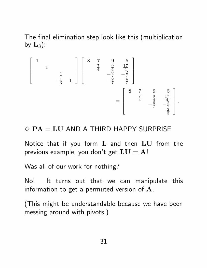
The final elimination step look like this (multiplicationby L3):

1

1

1

−13 1

8 7 9 574

94

174

−67 −2

7−2

747

=

8 7 9 5

74

94

174

−67 −2

723

.

3 PA = LU AND A THIRD HAPPY SURPRISE

Notice that if you form L and then LU from theprevious example, you don’t get LU = A!

Was all of our work for nothing?

No! It turns out that we can manipulate thisinformation to get a permuted version of A.

(This might be understandable because we have beenmessing around with pivots.)

31

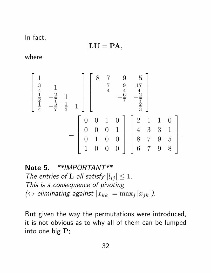
In fact,LU = PA,

where

134 112 −2

7 114 −3

713 1

8 7 9 574

94

174

−67 −2

723

=

0 0 1 0

0 0 0 1

0 1 0 0

1 0 0 0

2 1 1 0

4 3 3 1

8 7 9 5

6 7 9 8

.

Note 5. **IMPORTANT**The entries of L all satisfy |lij| ≤ 1.This is a consequence of pivoting(↔ eliminating against |xkk| = maxj |xjk|).

But given the way the permutations were introduced,it is not obvious as to why all of them can be lumpedinto one big P;

32

i.e.,L3P3L2P2L1P1A = U.

Here is where we use a third stroke of good luck:

These (elementary) operations can be reordered asfollows:

L3P3L2P2L1P1 = L′3L′2L′1P3P2P1,

where L′k =(Lk with subdiagonal entries permuted).

To be precise,

L′3 = L3,

L′2 = P3L2P−13 ,

L′1 = P3P2L1P−12 P−13 .

Note 6. Each Pj has j > k for Lk.=⇒ L′k has the same structure of Lk! (verify!)

33

Thus,

L′3L′2L′1P3P2P1 = L3(P3L2P

−13 )(P3P2L1P

−12 P

−13 )P3P2P1

= L3P3L2P2L1P1.

In the general m×m case, Gaussian elimination withpartial pivoting can be written as

(L′m−1 . . .L′2L′1)(Pm−1 . . .P2P1)A = U,

where

L′k = Pm−1 . . .Pk+1LkP−1k+1 . . .P

−1m−1.

Now we write

L = (L′m−1 . . .L′2L′1)−1

andP = (Pm−1 . . .P2P1)

to getPA = LU.

34

Note 7. In general, any square matrix (whether non-singular or not) has a factorization PA = LU, whereP is a permutation matrix, L is unit lower-triangularand whose elements satisfy |lij| ≤ 1, and U is upper-triangular.

Despite this being a bit of an abuse, this factorizationis really what is meant by the LU factorization of A.

The formula PA = LU has another greatinterpretation:

If you could permute A ahead of time using matrix P,then you could apply Gaussian elimination to A andyou would not need pivoting!

Of course, this cannot be done in practice because Pis not known a priori.

See lugui.m

See also pivotgolf.m

35

Solution of Banded Systems

Banded systems arise fairly often in practice; they canbe solved by a streamlined version Gaussian eliminationthat only operates within the bandwidth.

In fact, the streamlined solution of tridiagonal systemsby (pure) Gaussian elimination is occasionally calledthe Thomas algorithm.

In general, a solver would need to be told that theinput coefficient matrix A is banded, but Matlabcan detect bandedness automatically.

We now explore the algorithm to solve a tridiagonallinear system by Gaussian elimination with pivoting.

Note: Complete pivoting destroys the bandedness,causing fill-in, but partial pivoting preserves it.

Fill-in refers to the creation of non-zero elements where(structurally) zero elements used to be; it is undesirablebecause the newly created elements must be stored andoperated on (they are generally not zero!).

36

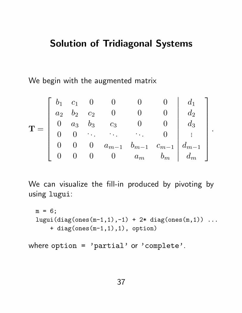
Solution of Tridiagonal Systems

We begin with the augmented matrix

T =

b1 c1 0 0 0 0 d1a2 b2 c2 0 0 0 d20 a3 b3 c3 0 0 d30 0 . . . . . . . . . 0 ...

0 0 0 am−1 bm−1 cm−1 dm−10 0 0 0 am bm dm

.

We can visualize the fill-in produced by pivoting byusing lugui:

m = 6;

lugui(diag(ones(m-1,1),-1) + 2* diag(ones(m,1)) ...

+ diag(ones(m-1,1),1), option)

where option = ’partial’ or ’complete’.

37

The Thomas Algorithm

We now present a rendition of the Thomas algorithmwithout pivoting (for simplicity).

The key to the algorithm is to notice that every stepof Gaussian elimination works on a system like

bixi + cixi+1 = di,

ai+1xi + bi+1xi+1 + ci+1xi+2 = di+1.

Zeroing below the diagonal only involves one elementand requires a multiplier −ai+1/bi, so that the nextsystem to solve is

b̃i+1xi+1 + ci+1xi+2 = d̃i+1,

ai+2xi+1 + bi+2xi+2 + ci+2xi+3 = di+2,

where b̃i+1 = bi+1−ai+1ci/bi and d̃i+1 = di+1−ai+1di/bi.

38

The Thomas Algorithm

Thus, the new system is of the same form as theprevious one, so the procedure can be repeated.

This leads to the following algorithm:

% forward substitution

b̃1 = b1; d̃1 = d1;

for i = 2:m,

l = ai/b̃i−1;

b̃i = bi − l ci−1;

d̃i = di − l d̃i−1;

% backward substitution

xm = d̃m/b̃m;

for i = m-1:-1:1,

xi = (d̃i − ci xi−1)/b̃i;

39

The Thomas Algorithm

In practice, the “tilde” variables are not stored; theoriginal variables are over-written.

To avoid additionally complicating the translation ofthe algorithm to code, we are not storing the multipliersl, but they could easily be stored in the lower diagonal.

See

thomasAlgorithmDemo.m

40

2.6 Why Is Pivoting Necessary?

Recall, the diagonal elements of U are called pivots.

Formally, the kth pivot is the coefficient of the kthvariable in the kth equation at the kth step of theelimination.

Both the computation of the multipliers and the backsubstitution require divisions by the pivots.

So, Gaussian elimination fails if any of the pivots arezero, but the problem may still have a perfectly welldefined solution.

It is a also bad idea to complete the computation ifany of the pivots are nearly zero!

To see what bad things can happen, consider a smallmodification to the problem 10 −7 0

−3 2 6

5 −1 5

x1x2x3

=

746

.41

This problem has the exact solution x = (0,−1, 1)T .

Change a22 from 2 to 2.099.

Note: Also change b2 so that the exact solution is stillx = (0,−1, 1)T .

10 −7 0

−3 2.099 6

5 −1 5

x1x2x3

=

7

3.901

6

.Suppose our computer does floating-point arithmeticwith 5 significant digits.

The first step of the elimination produces

10.000 −7.0000 0.0000

0.0000 −0.0010 6.0000

0.0000 2.5000 5.0000

x̂1

x̂2

x̂3

=

7.0000

6.0010

2.5000

.

The (2, 2) element is now quite small compared withthe other elements in the matrix.

42

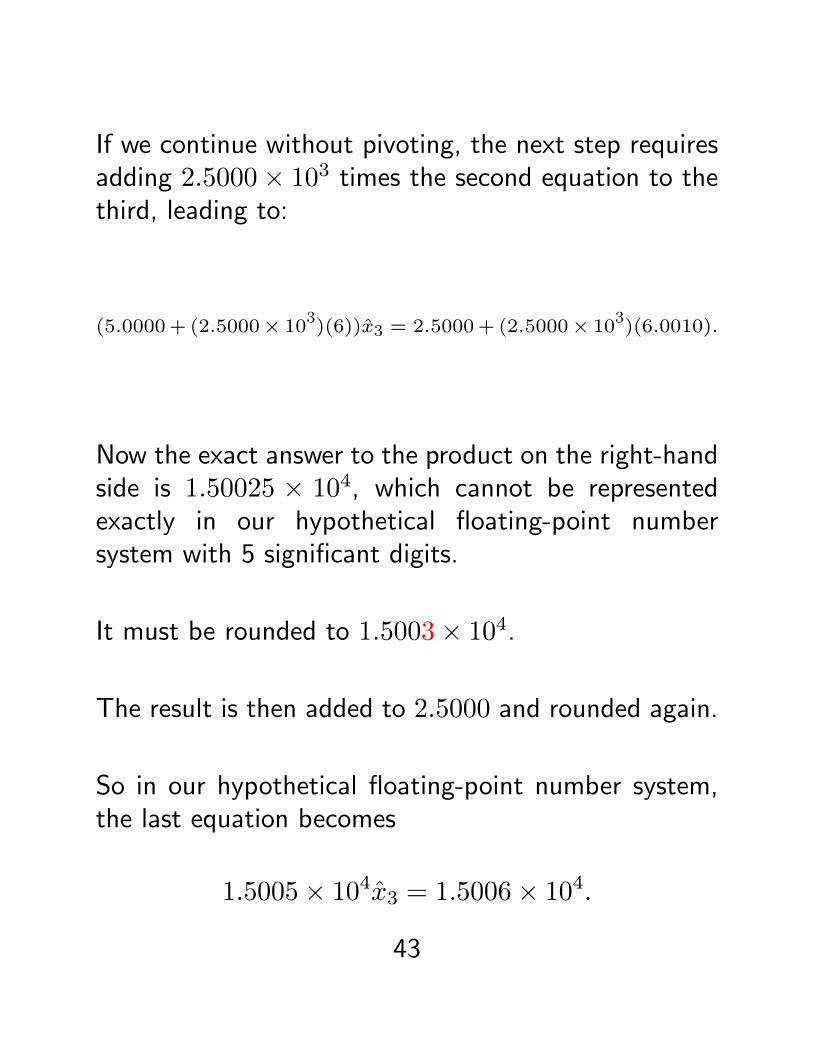
If we continue without pivoting, the next step requiresadding 2.5000× 103 times the second equation to thethird, leading to:

(5.0000+ (2.5000× 103)(6))x̂3 = 2.5000+ (2.5000× 10

3)(6.0010).

Now the exact answer to the product on the right-handside is 1.50025 × 104, which cannot be representedexactly in our hypothetical floating-point numbersystem with 5 significant digits.

It must be rounded to 1.5003× 104.

The result is then added to 2.5000 and rounded again.

So in our hypothetical floating-point number system,the last equation becomes

1.5005× 104x̂3 = 1.5006× 104.

43

The back substitution begins with

x̂3 =1.5006× 104

1.5005× 104= 1.0001.

Because x3 = 1, the error is not too serious.

However, x̂2 is determined from

−0.00100x̂2 + (6.0000)(1.0001) = 6.0010

=⇒ x̂2 =0.00040

−0.00100= −0.40000.

Finally x̂1 is determined from

10.000x̂1 + (−7.0000)(−0.40000) = 7.0000 =⇒ x̂1 = −0.42000.

Instead of the exact solution x = (0,−1, 1)T , we getthe approximation x̂ = (−0.42000,−0.40000, 1.0001)T !

What went wrong?

44

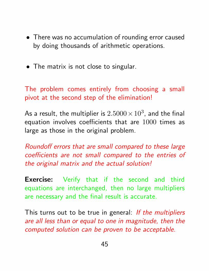
• There was no accumulation of rounding error causedby doing thousands of arithmetic operations.

• The matrix is not close to singular.

The problem comes entirely from choosing a smallpivot at the second step of the elimination!

As a result, the multiplier is 2.5000×103, and the finalequation involves coefficients that are 1000 times aslarge as those in the original problem.

Roundoff errors that are small compared to these largecoefficients are not small compared to the entries ofthe original matrix and the actual solution!

Exercise: Verify that if the second and thirdequations are interchanged, then no large multipliersare necessary and the final result is accurate.

This turns out to be true in general: If the multipliersare all less than or equal to one in magnitude, then thecomputed solution can be proven to be acceptable.

45

The multipliers can be guaranteed to be less than onein magnitude through the use of partial pivoting.

At the kth step of the forward elimination, the pivotis taken to be the element with the largest absolutevalue in the unreduced part of the kth column.

The row containing this pivot is then interchanged withthe kth row to bring the pivot element into the (k, k)position.

Of course, the same interchanges must be done withthe elements of b (otherwise we would be changingthe problem!).

The unknowns in x are not reordered because thecolumns of A are not interchanged.

46

2.8 The Effect of Roundoff Errors

Rounding errors always cause the computed solution x̂to differ from the exact solution, x = A−1b.

In fact, if the elements of x are not floating-pointnumbers themselves, then x̂ cannot equal x!

There are two common measures of the quality of x̂:

the error :e = x− x̂

and the residual :

r = b−Ax̂.

Matrix theory tells us that, because A is nonsingular,if one of these is 0, then so is the other.

But they may not both be “small” at the same time!

47

Consider the following example:[0.780 0.563

0.913 0.659

] [x1x2

]=

[0.217

0.254

].

Suppose we carry out Gaussian elimination with partialpivoting in three-digit arithmetic with truncation.

First, interchange the rows so that 0.913 is the pivot.

The multiplier is −0.780/0.913 = −0.854 (to 3 digits).

The elimination yields:[0.913 0.659

0 0.001

] [x̂1x̂2

]=

[0.254

0.001

].

Performing the back substitution:

x̂2 = 0.001/0.001 = 1.00 (exactly);

x̂1 = (0.254− 0.659)/0.913 = −0.443 (to 3 digits).

48

Thus the computed solution is x̂ = (−0.443, 1.000)T .

To assess the accuracy without knowing the exactanswer, we compute the residuals (exactly):

r = b−Ax̂ = (−0.000460,−0.000541)T .

The residuals are less than 10−3

→ it is hard to expect better on a 3-digit machine!

However, it is easy to see that the exact solution tothis system is x = (1.000,−1.000)T !

Our computed solution x̂ is so bad that the componentsactually have the wrong signs!

So why were our residuals so small?

Of course, this example is highly contrived: The matrixis very close to being singular (not typical of mostproblems in practice).

But we can still understand what happened.

49

If Gaussian elimination with partial pivoting is carriedout for this example on a computer with 6 or moredigits, the forward elimination will produce a systemsomething like[

0.913000 0.659000

0 0.000001

] [x̂1x̂2

]=

[0.254000

−0.000001

].

Notice that the sign of b2 differs from that obtainedwith 3-digit computation.

Now the back substitution produces

x̂2 = −0.000001/0.000001 = −1.00000,

x̂1 = (0.254− 0.659x̂2)/0.913 = 1.00000,

the exact answer!

Key point: On our 3-digit machine, x̂2 was computedby dividing two quantities, both on the order ofroundoff (and one of which did not even have thecorrect sign!).

50

Hence x̂2 can turn out to be almost anything.

Then this arbitrary value of x̂2 was substituted intothe first equation to obtain x̂1, essentially rendering itarbitrary as well.

We can reasonably expect the residual from the firstequation to be small: x̂1 was computed in such a wayas to make this certain.

Now comes a subtle but crucial point:

We can also expect the residual from the secondequation to be small, precisely because the equationsare almost multiples of each other!

→ Any pair (x̂1, x̂2) that nearly satisfies the firstequation will also nearly satisfy the second.

If the two equations really were multiples of eachother, we would not need the second equation at all:any solution of the first equation would automaticallysatisfy the second one.

This example is admittedly on the phony side, but theconclusion is not!

51

According to Cleve Moler, this is probably the singlemost important fact that we have learned aboutmatrix computation since the invention of the digitalcomputer:

Gaussian elimination with partial pivoting isguaranteed to produce small residuals.

“guaranteed” ↔ it is possible to prove a precisetheorem that bounds the size of the residual(assuming certain technical details about floating-pointarithmetic).

“small” ↔ on the order of roundoff error relative to:

• the size of the elements of A,

• the size of the elements of the matrix during theelimination process,

• the size of the elements of x.

52

If any of these are “large”, then the residual will notnecessarily be small in an absolute sense.

Final note: Even if the residual is small, this does notmean that the error will be small!

The relationship between the size of the residual andthe size of the error is partly determined by thecondition number of A (see next section).

53

2.9 Norms and Condition Numbers

The coefficients defining a system of linear equationsoften contain errors; e.g., experimental, roundoff, etc.

Even if the system can be stored exactly, roundofferrors will be introduced during the solution process.

It can be shown that roundoff errors in Gaussianelimination have the same effect on the answer aserrors in the original coefficients.

So the question becomes: if the coefficients are alteredslightly, how much is the solution altered?

Put another way, if Ax = b, what is the sensitivity ofx to changes in A and b?

The answer to this question we have to consider themeaning of “nearly singular” matrices.

If A is a singular matrix, then for some vectors b, asolution x will not exist, and for others it will not beunique.

54

So if A is nearly singular, we can expect small changesin A and b to cause very large changes in x.

On the other hand, if A = I, then x = b.

So if A is close to I, small changes in A and b shouldresult in correspondingly small changes in x.

It might appear that there is some connection betweenthe size of the pivots encountered in Gaussianelimination with partial pivoting and nearness tosingularity: if arithmetic is exact, all pivots wouldbe nonzero if and only if the matrix is nonsingular.

To some extent, it is also true that if the “partial”pivots are small, then the matrix is close to singular.

However, in the presence of roundoff, the converse isno longer true: a matrix might be close to singulareven though none of the pivots are small .

In order to obtain a more precise quantification ofnearness to singularity, we need to introduce theconcept of a norm of a vector.

55

In general, the p-norm of a vector x is denoted by‖x‖p; it is a scalar that measures the “size” of x.

The family of vector norms known as lp is defined by

‖x‖p =

(m∑i=1

|xi|p)1/p

, 1 ≤ p <∞.

In practice, we only use:

• p = 1 (Manhattan or taxicab norm)

• p = 2 (Euclidean norm)

• p→∞ (Chebyshev or maximum norm)

All three norms are easy to compute, and they satisfy

‖ · ‖1 ≥ ‖ · ‖2 ≥ ‖ · ‖∞.

Often, the specific value of p is not important, and wesimply write ‖x‖.

56

All vector norms satisfy the following relations,associated with the interpretation it being a distance:

• ‖x‖ > 0 with ‖x‖ = 0 ⇐⇒ x = 0.

• ‖cx‖ = |c|‖x‖ for all scalars c.

• ‖x+ y‖ ≤ ‖x‖+ ‖y‖ (triangle inequality).

The first relation says that the size of a non-zero vectoris positive.

The second relations says that if a vector is scaled bya factor c then its size is also scaled by c.

The triangle inequality is a generalization of the factthat the size of one side of a triangle cannot exceedthe sum of the sizes of the other two sides.

A useful variant of the triangle inequality is

‖x− y‖ ≥ ‖x‖ − ‖y‖.

57

In Matlab, ‖x‖p is computed by norm(x,p);norm(x) defaults to norm(x,2).

See normDemo.m

Multiplication of a vector x by a matrix A results in anew vector Ax that can be very different from x.

In particular, the change in norm is directly related tothe sensitivity we want to measure.

The range of the possible change can be expressed bythe quantities:

M = maxx 6=0

‖Ax‖‖x‖

, m = minx 6=0

‖Ax‖‖x‖

.

Note: If A is singular, m = 0.

The ratio M/m is called the condition number of A:

κ(A) =M

m.

58

The precise numerical value of κ(A) depends on thevector norm being used!

Normally we are only interested in order of magnitudeestimates of the condition number, so the particularnorm is usually not very important.

Consider the linear system

Ax = b

and a perturbed system

A(x+ δx) = (b+ δb).

We think of δb as the error in b and δx as the resultingerror in x.

(We don’t necessarily assume that the errors are small!)

Note: A(δx) = δb.

59

The definitions of M and m imply

‖b‖ ≤M‖x‖, ‖δb‖ ≥ m‖δx‖.

So if m 6= 0,

‖δx‖‖x‖

≤ κ(A)‖δb‖‖b‖

.

Thus, the condition number is a relative errormagnification factor .

In other words, relative changes in b can cause relativechanges in x that are κ(A) times as large.

It turns out that the same is true of changes in A.

κ(A) is also a measure of nearness to singularity:→ if κ(A) is large, A is close to singular .

60

Some basic properties of the condition number:

• M ≥ m, so κ(A) ≥ 1.

• If P is a permutation matrix, then Px is simply arearrangement of x, so ‖Px‖ = ‖x‖ for all x; henceκ(P) = 1. In particular, κ(I) = 1.

• If A is multiplied by a scalar c, then M and m areboth multiplied by c, so κ(cA) = κ(A).

• If D is a diagonal matrix, then κ(D) = max |dii|min |dii|

.

These last two properties are reasons that κ(A) is abetter measure of nearness to singularity than det(A).

e.g., consider a 100× 100 diagonal matrix with 0.1 onthe diagonal.

Then det(A) = 10−100 → generally a small number!

But κ(A) = 1, and in fact for linear systems ofequations, such a matrix behaves more like I than likea singular matrix.

61

Example

Let

A =

[4.1 2.8

9.7 6.6

], b =

[4.1

9.7

].

The solution to Ax = b is x = (1, 0)T .

In the 1-norm, ‖b‖1 = 13.8, and ‖x‖1 = 1.

If we perturb the right-hand side to b̃ = (4.11, 9.70)T ,then the solution becomes x̃ = (0.34, 0.97)T .

→ A tiny perturbation has completely changed thesolution!

Defining δb = b− b̃ and δx = x− x̃, we find

‖δb‖1 = 0.01, ‖δx‖1 = 1.63.

62

Thus,

‖δb‖1‖b‖1

= 0.0007246,‖δx‖1‖x‖1

= 1.63,

and so

κ(A) ≥ 1.63

0.0007246= 2249.4.

(We have made it so that in fact cond(A,1)= 2249.4.)

Important note: This example deals with the exactsolutions to two slightly different problems.

→ The method to obtain the solutions is irrelevant!

The example is chosen so that the effect of changingb is quite pronounced, but similar behaviour can beexpected in any problem with a large condition number.

Now we see how κ(A) also plays a fundamental rolein the analysis of roundoff errors during Gaussianelimination.

Assume that A and b have elements that are exactfloating-point numbers.

63

Let x be the exact solution, and let x∗ be the vectorof floating-point numbers obtained from Gaussianelimination representing the computed solution.

Assume A is non-singular and nothing funny happenedlike underflows or overflows during the elimination.

Then it is possible to establish the followinginequalities:

‖b−Ax∗‖‖A‖‖x‖

≤ ρεmachine,‖x− x∗‖‖x∗‖

≤ ρκ(A)εmachine,

where ρ is a constant (rarely larger than about 10) and‖A‖ is the norm of A (to be defined momentarily).

But first, what do these inequalities say?

The first one says that the norm of the relative residualis about the size of roundoff error — no matter howbadly conditioned the matrix is!

(See example in the previous section.)

64

The second one says that the norm of the relative errorwill be small if κ(A) is small — but it might be quitelarge if κ(A) is large, i.e., if A is nearly singular !

Now back to defining the matrix norm.

The norm of a matrix A is defined to be

‖A‖ = maxx 6=0

‖Ax‖‖x‖

.

Technically this is called an induced matrix normbecause it is defined using an underlying vector norm.

(Other matrix norms do exist, but we do not considerthem in this course.)

It turns out that ‖A−1‖ = 1/m, so an equivalentdefinition of the condition number of a matrix isκ(A) = ‖A‖‖A−1‖.

Note: The precise numerical values of ‖A‖ and κ(A)depend on the underlying vector norm.

65

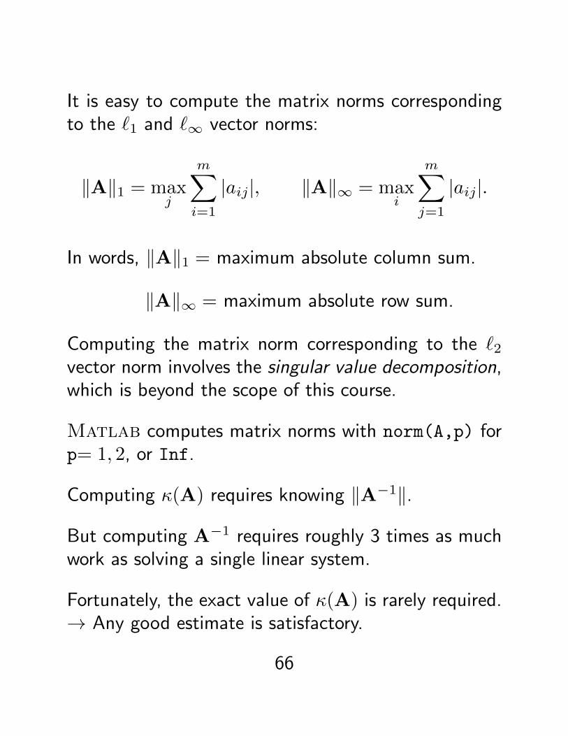
It is easy to compute the matrix norms correspondingto the `1 and `∞ vector norms:

‖A‖1 = maxj

m∑i=1

|aij|, ‖A‖∞ = maxi

m∑j=1

|aij|.

In words, ‖A‖1 = maximum absolute column sum.

‖A‖∞ = maximum absolute row sum.

Computing the matrix norm corresponding to the `2vector norm involves the singular value decomposition,which is beyond the scope of this course.

Matlab computes matrix norms with norm(A,p) forp= 1, 2, or Inf.

Computing κ(A) requires knowing ‖A−1‖.

But computing A−1 requires roughly 3 times as muchwork as solving a single linear system.

Fortunately, the exact value of κ(A) is rarely required.→ Any good estimate is satisfactory.

66

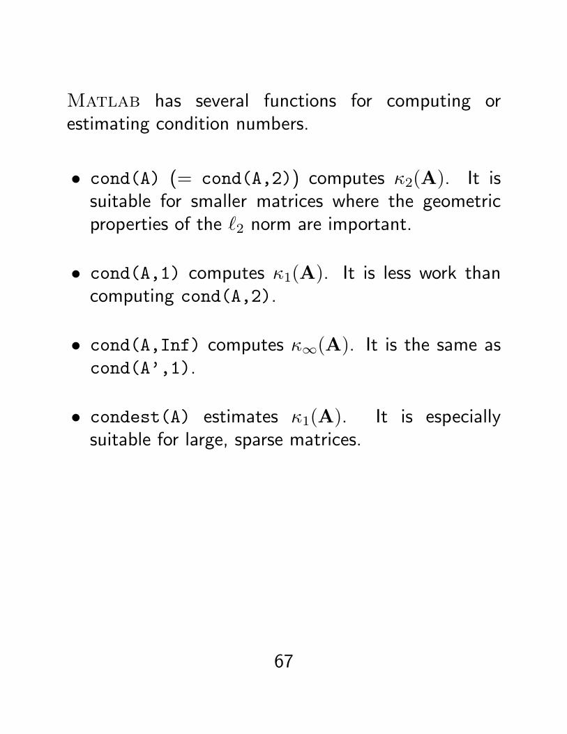
Matlab has several functions for computing orestimating condition numbers.

• cond(A) (= cond(A,2)) computes κ2(A). It issuitable for smaller matrices where the geometricproperties of the `2 norm are important.

• cond(A,1) computes κ1(A). It is less work thancomputing cond(A,2).

• cond(A,Inf) computes κ∞(A). It is the same ascond(A’,1).

• condest(A) estimates κ1(A). It is especiallysuitable for large, sparse matrices.

67