chapter 2 lagrangian and eulerian finite elements in one
TRANSCRIPT

T. Belytschko, Chapter 2, December 16, 1998
CHAPTER 2LAGRANGIAN AND EULERIAN FINITE
ELEMENTS IN ONE DIMENSION
by Ted BelytschkoNorthwestern University@ Copyright 1997
2.1 Introduction
In this chapter, the equations for one-dimensional models of nonlinear continua aredescribed and the corresponding finite element equations are developed. The developmentis restricted to one dimension to simplify the mathematics so that the salient features ofLagrangian and Eulerian formulations can be demonstrated easily. These developments areapplicable to nonlinear rods and one-dimensional phenomena in continua, including fluidflow. Both Lagrangian and Eulerian meshes will be considered. Two commonly usedtypes of Lagrangian formulations will be described: updated Lagrangian and totalLagrangian. In the former, the variables are expressed in the current (or updated)configuration, whereas in the latter the variables are expressed in terms of the initialconfiguration. It will be seen that a variety of descriptions can be developed for largedeformation problems. The appropriate description depends on the characteristics of theproblem to be solved.
In addition to describing the several types of finite element formulations for nonlinearproblems, this Chapter reviews some of the concepts of finite element discretization andfinite element procedures. These include the weak and strong forms, the operations ofassembly, gather and scatter, and the imposition of essential boundary conditions and initialconditions. Mappings between different coordinate systems are discussed along with theneed for finite element mappings to be one-to-one and onto. Continuity requirements ofsolutions and finite element approximations are also considered. While much of thismaterial is familiar to most who have studied linear finite elements, they are advised to atleast skim this Chapter to refresh their understanding.
In solid mechanics, Lagrangian meshes are most popular. Their attractiveness stemsfrom the ease with which they handle complicated boundaries and their ability to followmaterial points, so that history dependent materials can be treated accurately. In thedevelopment of Lagrangian finite elements, two approaches are commonly taken:
1. formulations in terms of the Lagrangian measures of stress and strain in whichderivatives and integrals are taken with respect to the Lagrangian (material)coordinates X, called total Lagrangian formulations
2. formulations expressed in terms of Eulerian measures of stress and strain inwhich derivatives and integrals are taken with respect to the Eulerian (spatial)coordinates x, often called updated Lagrangian formulations.
Both formulations employ a Lagrangian mesh, which is reflected in the term Lagrangian inthe names.
Although the total and updated Lagrangian formulations are superficially quitedifferent, it will be shown that the underlying mechanics of the two formulations isidentical; furthermore, expressions in the total Lagrangian formulation can be transformedto updated Lagrangian expressions and vice versa. The major difference between the two
2-1

T. Belytschko, Chapter 2, December 16, 1998
formulations is in the point of view: the total Lagrangian formulation refers quantities tothe original configuration, the updated Lagrangian formulation to the current configuration,often called the deformed configuration. There are also differences in the stress anddeformation measures which are typically used in these two formulations. For example,the total Lagrangian formulation customarily uses a total measure of strain, whereas theupdated Lagrangian formulation often uses a rate measure of strain. However these are notinherent characteristics of the formulations, for it is possible to use total measures of strainin updated Lagrangian formulations, and rate measures in total Lagrangian formulation.These attributes of the two Lagrangian formulations are discussed further in Chapter 4.
Until recently, Eulerian meshes have not been used much in solid mechanics. Eulerianmeshes are most appealing in problems with very large deformations. Their advantage inthese problems is a consequence of the fact that Eulerian elements do not deform with thematerial. Therefore, regardless of the magnitudes of the deformation in a process, Eulerianelements retain their original shape. Eulerian elements are particularly useful in modelingmany manufacturing processes, where very large deformations are often encountered.
For each of the formulations, a weak form of the momentum equation, which isknown as the principle of virtual work (or virtual power) will be developed. The weakform is developed by taking the product of a test function with the governing partialdifferential equation, the momentum equation. The integration is performed over thematerial coordinates for the total Lagrangian formulation, over the spatial coordinates forthe Eulerian and updated Lagrangian formulation. It will also be shown how the tractionboundary conditions are treated so that the approximate (trial) solutions need not satisfythese boundary conditions exactly. This procedure is identical to that in linear finiteelement analysis. The major difference in geometrically nonlinear formulations is the needto define the coordinates over which the integrals are evaluated and to specify the choice ofstress and strain measures.
The discrete equations for a finite element approximation will then be derived. Forproblems in which the accelerations are important (often called dynamic problems) or thoseinvolving rate-dependent materials, the resulting discrete finite element equations areordinary differential equations (ODEs). The process of discretizing in space is called asemidiscretization since the finite element procedure only converts the spatial differentialoperators to discrete form; the derivatives in time are not discretized. For static problemswith rate-independent materials, the discrete equations are independent of time, so the finiteelement discretization results in a set of nonlinear algebraic equations.
Examples of the total and updated Lagrangian formulations are given for the 2-node,linear displacement and 3-node, quadratic displacement elements. Finally, to enable thestudent to solve some nonlinear problems, a central difference explicit time-integrationprocedures is described.
2.2 Governing Equations For Total Lagrangian Formulation
Nomenclature. Consider the rod shown in Fig. 1. The initial configuration, alsocalled the undeformed configuration of the rod, is shown in the top of the figure. Thisconfiguration plays an important role in the large deformation analysis of solids. It is alsocalled the reference configuration, since all equations in the total Lagrangian formulationare referred to this configuration. The current or deformed configuration is shown at thebottom of the figure. The spatial (Eulerian) coordinate is denoted by x and the coordinatesin the reference configuration, or material (Lagrangian) coordinates, by X . The initialcross-sectional area of the rod is denoted by A0 X( ) and its initial density by ρ0 X( );
2-2

T. Belytschko, Chapter 2, December 16, 1998
variables pertaining to the reference (initial, undeformed) configuration will always beidentified by a subscript or superscript nought. In this convention, we could indicate thematerial coordinates by x0 since they correspond to the initial coordinates of the materialpoints, but this is not consistent with most of the continuum mechanics literature, so wewill always use X for the material coordinates.
The cross-sectional area in the deformed state is denoted by A X, t( ) ; as indicated, it isa function of space and time. The spatial dependence of this variable and all others isexpressed in terms of the material coordinates. The density is denoted by ρ X ,t( ) and thedisplacement by u X ,t( ) . The boundary points in the reference configuration are Xa andXb .
XX
ab
bXX
x
xab = ( , t )
A(X) = A(x)_
A (X)o
x , X
T
T
Fig. 1.1. The undeformed (reference) configuration and deformed (current) configurations for a one-dimensional rod loaded at the left end; this is the model problem for Sections 2.2 to 2.8.
Deformation and Strain Measure. The variables which specify the deformation andthe stress in the body will first be described. The motion of the body is described by afunction of the Lagrangian coordinates and time which specifies the position of eachmaterial point as a function of time:
x = φ X ,t( ) X ∈ Xa , Xb[ ] (2.2.1)
where φ X, t( ) is called a deformation function. This function is often called a map betweenthe initial and current domains. The material coordinates are given by the deformationfunction at time t = 0, so
X =φ X , 0( ) (2.2.2)
As can be seen from the above, the deformation function at t = 0 is the identity map.
The displacement u X , t( ) is given by the difference between the current position andthe original position of a material point, so
u X , t( ) = φ X , t( ) − X or u = x − X (2.2.3)
The deformation gradient is defined by
2-3

T. Belytschko, Chapter 2, December 16, 1998
F =∂φ∂X
=∂x
∂X(2.2.4)
The second definitions in Eq. (2.2.3) and (2.2.4) can at times be ambiguous. Forexample, Eq. (2.2.4) appears to involve the partial derivative of an independent variable xwith respect to another independent variable X , which is meaningless. Therefore, itshould be understood that whenever x appears in a context that implies it is a function, thedefinition x = φ X ,t( ) is implied.
Let J be the Jacobian between the current and reference configurations. The Jacobianis usually defined by J( x( X) ) = ∂x / ∂X for one-dimensional mappings; however, tomaintain consistency with multi-dimensional formulations of continuum mechanics, wewill define the Jacobian as the ratio of an infinitesimal volume in the deformed body, A∆x ,to the corresponding volume of the segment in the undeformed body A0∆X , so it is givenby
J = ∂x∂X
A
A0
=FA
A0
(2.2.5)
The deformation gradient F is an unusual measure of strain since its value is one whenthe body is undeformed. We will therefore define the measure of strain by
ε X, t( ) = F X, t( )–1≡ ∂x
∂X–1= ∂u
∂X(2.2.6)
so that it vanishes in the undeformed configuration. There are many other measures ofstrain, but this is the most convenient for this presentation. This measure of straincorresponds to what is known as the stretch tensor in multi-dimensional problems. In onedimension, it is equivalent to the engineering strain.
Stress Measure. The stress measure which is used in total Lagrangian formulationsdoes not correspond to the well known physical stress. To explain the measure of stress tobe used, we will first define the physical stress, which is also known as the Cauchy stress.Let the total force across a given section be denoted by T and assume that the stress isconstant across the cross-section. The Cauchy stress is given by
σ = TA (2.2.7)
This measure of stress refers to the current area A. In the total Lagrangian formulation, wewill use the nominal stress. The nominal stress will be denoted by P and is given by
P = TA0
(2.2.8)
It can be seen that it differs from the physical stress in that the net resultant force is dividedby the initial, or undeformed, area A0 . This is equivalent to the definition of engineeringstrain; however, in multi-dimensions, the nominal stress is not equivalent to theengineering stress, this is discussed further in Chapter 3.
2-4

T. Belytschko, Chapter 2, December 16, 1998
Comparing Eqs. (2.2.7) and (2.2.8), it can be seen that the physical and nominalstresses are related by
σ =A0A P P = A
A0σ (2.2.9)
Therefore, if one of the stresses is known, the other can always be computed if the currentand initial cross-sectional areas are known.
Governing Equations. The nonlinear rod is governed by the following equations:
1. conservation of mass;2. conservation of momentum;3. conservation of energy;4. a measure of deformation, often called a strain-displacement equation;5. a constitutive equation, which describes material behavior and relates stress to a
measure of deformation;
In addition, we require the deformation to be continuous, which is often called acompatibility requirement. The governing equations and initial and boundary conditionsare summarized in Box 1.
Conservation of mass. The equation for conservation of mass for a Lagrangianformulation can be written as (see Appendix A for an engineering derivation):
ρJ = ρ0J0 or ρ X ,t( )J X, t( ) = ρ0 X( )J0 X( ) (2.2.10)
where the second expression is given to emphasize that the variables are treated asfunctions of the Lagrangian coordinates. Conservation of matter is an algebraic equationonly when expressed in terms of material coordinates. Otherwise, it is a partial differentialequation. For the rod, we can use Eq. (2.2.4) to write Eq. (2.2.5) as
ρFA= ρ0A0 (2.2.11)
where we have used the fact that J0 = 1.
Conservation of momentum. Conservation of momentum is written in terms of thenominal stress and the Lagrangian coordinates as (a derivation is given in Appendix A):
A0P( ),X +ρ0 A0b = ρ0 A0˙ u (2.2.12)
where the superposed dots denote the material time derivative. The material time derivative
of the velocity, the acceleration, is written as D2u Dt2 . The subscript following a commadenotes partial differentiation with respect to that variable, i.e.
P X, t( ),X ≡ ∂P( X, t)
∂X(2.2.13)
Equation (2.2.12) is called the momentum equation, since it represents conservationof momentum. If the initial cross-sectional area is constant in space, the momentumequation becomes
2-5

T. Belytschko, Chapter 2, December 16, 1998
P, X +ρ0b = ρ0˙ u (2.2.14)
Equilibrium Equation. When the inertial term ρ0˙ u vanishes, i.e. when the problem isstatic, the momentum equation becomes the equilibrium equation
A0P( ) ,X + ρ0A0b = 0 (2.2.15)
Solutions of the equilibrium equations are called equilibrium solutions. Some authors callthe momentum equation an equilibrium equation regardless of whether the inertial term isnegligible; since equilibrium usually connotes a body at rest or moving with constantvelocity, this nomenclature is avoided here.
Energy Conservation. The energy conservation equation for a rod of constant area isgiven by
ρ0˙ w int = ˙ F P− qx,X + ρ0 s (2.2.16)
where qx is the heat flux, s is the heat source per unit mass and ˙ w int is the rate of change ofinternal energy per unit mass. In the absence of heat conduction or heat sources, theenergy equation gives
ρ0 ˙ w int = ˙ F P (2.2.17)
which shows that the internal work is given by the product of the rate of the deformation Fand the nominal stress P. The energy conservation equation is not needed for the treatmentof isothermal, adiabatic processes.
Constitutive Equations. The constitutive equations reflect the stresses which aregenerated in the material as a response to deformation. The constitutive equations relate thestress to the measures of strain at a material point. The constitutive equation can be writteneither in total form, which relates the current stress to the current deformation
P X,t( ) = SPF F X, t ( ), ˙ F X, t ( ), etc., t ≤ t( ) (2.2.18)
or in rate form
˙ P X,t( ) = StPF ˙ F X, t ( ), F x,t ( ), P X, t ( ), etc., t ≤ t( ) (2.2.19)
Here SPF and StPF are functions of the deformation which give the stress and stress rate,
respectively. The superscripts are here appended to the constitutive functions to indicatewhich measures of stress and strain they relate.
As indicated in Eq. (2.2.18), the stress can depend on both F and F and on other statevariables, such as temperature, porosity; “etc.” refers to these additional variables whichcan influence the stress. The prior history of deformation can also affect the stress, as in anelastic-plastic material; this is explicitly indicated in Eqs. (2.2.18-2.2.19) by letting theconstitutive functions depend on deformations for all time prior to t. The constitutiveequation of a solid is expressed in material coordinates because the stress in a solid usually
2-6

T. Belytschko, Chapter 2, December 16, 1998
depends on the history of deformation at that material point. For example, in an elasticsolid, the stress depends on strain at the material point. If there are any residual stresses,these stresses are frozen into the material and move with the material point. Therefore,constitutive equations with history dependence should track material points and are writtenin terms of the material coordinates. When a constitutive equation for a history dependentmaterial is written in terms of Eulerian coordinates, the motion of the point must beaccounted for in the evaluation of the stresses, which will be discussed in Chapter 7.
The above functions should be continuos functions of the independent variables.Preferably they should be continuously differentiable, for otherwise the stress is lesssmooth than the displacements, which can cause difficulties.
Examples of constitutive equations are:
(a) linear elastic material:
total form: P X, t( ) = EPFε( X ,t ) = EPF F X ,t( )–1( ) (2.2.20)
rate form: ˙ P X ,t( ) = EPF ˙ ε ( X, t) = EPF ˙ F X ,t( ) (2.2.21)
(b) linear viscoelastic
P X, t( ) = EPF F X ,t( )–1( ) +α ˙ F X ,t( )[ ]or P = E PF( ε + α˙ ε ) (2.2.22)
For small deformations the material parameter EPF corresponds to Young’s modulus; theconstant α determines the magnitude of damping.
Momentum equation in terms of displacements. A single governing equation forthe rod can be obtained by substituting the relevant constitutive equation, i.e. (2.2.18) or(2.2.19), into the momentum equation (2.2.12) and expressing the strain measure in termsof the displacement by (2.2.6). For the total form of the constitutive equation (2.2.18), theresulting equation can be written as
A0P u,X , ˙ u , X ,. .( )( ),X
+ ρ0 A0b = ρ0A0˙ u (2.2.23)
which is a nonlinear partial differential equation (PDE) in the displacement u(X,t). Thecharacter of this partial differential equation is not readily apparent from the above anddepends on the details of the constitutive equation. To illustrate one form of this PDE, weconsider a linear elastic material. For a linear elastic material, Eq. (2.2.20), the constitutiveequation and (2.2.23) yield
A0EPFu, X( ),X
+ ρ0A0b = ρ0 A0˙ u (2.2.24)
It can be seen that in this PDE, the highest derivatives with respect to the materialcoordinate X is second order, and the highest derivative with respect to time is also secondorder, so the PDE is second order in X and time t. If the stress in the constitutive equationonly depends on the first derivatives of the displacements with respect to X and t asindicated in (2.2.18) and (2.2.19), then the momentum equation will similarly be a secondorder PDE in space and time.
2-7

T. Belytschko, Chapter 2, December 16, 1998
For a rod of constant cross-section and modulus, if the body force vanishes, i.e. whenb = 0, the momentum equation for a linear material becomes the well known linear waveequation
u,XX = 1
c2 ˙ u (2.2.25)
where c is the wave speed relative to the undeformed configuration and given by
c2 = EPF
ρ0(2.2.26)
Boundary Conditions. The independent variables of the momentum equation are thecoordinate X and the time t. It is an initial-boundary value problem (IBVP). To completethe description of the IBVP, the boundary conditions and initial conditions must be given.The boundary in a one dimensional problem consists of the two points at the ends of thedomain, which in the model problem are the points Xa and Xb . From the linear form ofthe momentum equations, Eq. (2.2.23), it can be seen that the partial differential equation issecond order in X. Therefore, at each end, either u or u,X must be prescribed as a boundary
condition. In solid mechanics, instead of u,X, the traction t x0 = n0 P is prescribed; n0 is the
unit normal to the body which is given by n0 = 1 at Xa, n0 = −1 at Xb. Since the stress is afunction of the measure of strain, which in turn depends on the derivative of the
displacement by Eq. (2.2.6), prescribing tx0 is equivalent to prescribing u,X; the superscript
"naught" on t indicates that the traction is defined over the undeformed area; the superscript
is always explicitly included on the traction tx0 to distinguish it from the time t. Therefore
either the traction or the displacement must be prescribed at each boundary.
A boundary is called a displacement boundary and denoted by Γu if the displacementis prescribed; it is called a traction boundary and denoted by Γt if the traction is prescribed.The prescribed values are designated by a superposed bar. The boundary conditions are
u = u on Γu (2.2.27)
n0P = tx0
on Γt (2.2.28)
As an example of the boundary conditions in solid mechanics, for the rod in Fig. 2.1, theboundary conditions are
u(Xa,t) = 0 n0 Xb( )P Xb , t( ) = P Xb , t( ) = T t( )
A0 Xb( ) (2.2.29)
The traction and displacement cannot be prescribed at the same point, but one of thesemust be prescribed at each boundary point; this is indicated by
Γu ∩Γ t = 0 Γu ∪Γt = Γ (2.2.30)
2-8

T. Belytschko, Chapter 2, December 16, 1998
Thus in a one dimensional solid mechanics problem any boundary is either a tractionboundary or a displacement boundary, but no boundary is both a prescribed traction andprescribed displacement boundary.
Initial Conditions. Since the governing equation for the rod is second order in time,two sets of initial conditions are needed. We will express the initial conditions in terms ofthe displacements and velocities:
u X, 0( ) = u0 X( ) for X ∈ Xa,X b[ ] (2.2.31a)
˙ u X, 0( ) = v0 X( ) for X ∈ Xa ,Xb[ ] (2.2.31b)
If the body is initially undeformed and at rest, the initial conditions can be written as
u X, 0( ) = 0 u X , 0( ) = 0 (2.2.32)
Jump Conditions. In order for the derivative in Eq.(2.2.12) to exist, the quantity A0Pmust be continuous. However, neither A0 nor P need be continuous in the entire interval.Therefore momentum balance requires that
A0P = 0 (2.2.33)
where ⟨f⟩ designates the jump in f(X), i.e.
f X( ) = f X + ε( )– f X – ε( ) ε → 0 (2.2.34)
In dynamics, it is possible to have jumps in the stress, known as shocks, which can eitherbe stationary or moving. Moving discontinuities are governed by the Rankine-Hugoniotrelations, but these are not considered in this Chapter.
2.3 Weak Form for Total Lagrangian Formulation
The momentum equation cannot be discretized directly by the finite element method. Inorder to discretize this equation, a weak form, often called a variational form, is needed.The principle of virtual work, or weak form, which will be developed next, is equivalent tothe momentum equation and the traction boundary conditions (2.2.33). Collectively, thesetwo equations are called the classical strong form. The weak form can be used toapproximate the strong form by finite elements; solutions obtained by finite elements areapproximate solutions to the strong form.
Strong Form to Weak Form. A weak form will now be developed for the momentumequation (2.2.23) and the traction boundary conditions. For this purpose we define trialfunctions u X ,t( ) which satisfy any displacement boundary conditions and are smoothenough so that all derivatives in the momentum equation are well defined. The testfunctions δu X( ) are assumed to be smooth enough so that all of the following steps arewell defined and to vanish on the prescribed displacement boundary. The weak form isobtained by taking the product of the momentum equation expressed in terms of the trialfunction with the test function. This gives
2-9

T. Belytschko, Chapter 2, December 16, 1998
δu A0P( ), X + ρ0 A0b– ρ0A0
˙ u [ ]X a
Xb
∫ dX = 0 (2.3.1)
Using the derivative of the product in the first term in (2.3.1) gives
δu
Xa
Xb
∫ ( A0P) ,X dX = δuA0P( ),X – δu,X A0P[ ]Xa
Xb∫ dX (2.3.2)
Applying the fundamental theorem of calculus to the above gives
δu A0P( ) , XX a
Xb∫ dX =– δu, X A0P( )Xa
X b∫ dX + δuA0n0P( )
Γ
= – δu, X A0P( )Xa
X b∫ dX + δuA0t x0( )
Γt
(2.3.3)
where we obtained the second line using the facts that the test function δu vanishes on theprescribed displacement boundary, the complementarity conditions on the boundaries(2.2.30) and the traction boundary conditions. Substituting (2.3.3) into the first term ofEq. (2.3.1) gives (with a change of sign)
δu, XA0 P – δu ρ0 A0b – ρ0 A0˙ u ( )[ ]
Xa
Xb
∫ dX – δuA0 t x0( )
Γ t
= 0 (2.3.4)
The above is the weak form of the momentum equation and the traction boundary conditionfor the total Lagrangian formulation.
Smoothness of Test and Trial functions; Kinematic Admissibility. We shallnow investigate the smoothness required to go through the above steps more closely. Forthe momentum equation (2.2.12) to be well defined in a classical sense, the nominal stressand the initial area must be continuously differentiable, i.e. C1; otherwise the firstderivative would have discontinuities. If the stress is a smooth function of the derivative ofthe displacement as in (2.2.18), then to obtain this continuity in the stresses requires thatthe trial functions must be C2 . For Eq. (2.3.2) to hold, the test function δu X( ) must be
C1 .
However, the weak form is well defined for test and trial functions which are far lesssmooth, and indeed the test and trial functions to be used in finite element methods will berougher. The weak form (2.3.4) involves only the first derivative of the test function andthe trial function appears directly or as a first derivative of the trial function through thenominal stress. Thus the integral in the weak form is integrable if both functions are C0 .
We will now define the conditions on the test and trial function more precisely. Theweak form is well-defined if the trial functions u(X,t) are continuous functions with
piecewise continuous derivatives, which is stated symbolically by u X ,t( ) ∈C0 X( ) , where
the X in the parenthesis following C0 indicates that it pertains to the continuity in X; notethat this definition permits discontinuities of the derivatives at discrete points. This is thesame as the continuity of finite element approximations in linear finite element procedures:
2-10

T. Belytschko, Chapter 2, December 16, 1998
the displacement is continuous and continuously differentiable within elements, but thederivative u,X is discontinuous across element boundaries. In addition, the trial functionu(X,t) must satisfy all displacement boundary conditions. These conditions on the trialdisplacements are indicated symbolically by
u X ,t( ) ∈U where U = u X, t( ) u X ,t( ) ∈ C0 X( ), u = u on Γu (2.3.5)
Displacement fields which satisfy the above conditions, i.e. displacements which are in U,are called kinematically admissible.
The test functions are denoted by δu(X); they are not functions of time. The testfunctions are required to be C0 in X and to vanish on displacement boundaries, i.e.,
δu X( ) ∈U0 where U0 = δu X( ) δ X( )u ∈C0 X( ), δu = 0 on Γu (2.3.6)
We will use the prefix δ for all variables which are test functions and for variables whichare related to test functions. This convention originates in variational methods, where thetest function emerges naturally as the difference between admissible functions. Although itis not necessary to know variational methods to understand weak forms, it provides anelegant framework for developing various aspects of the weak form. For example, invariational methods any test function is a variation and defined as the difference between
two trial functions, i.e. the variation δu(X) = ua(X) – ub(X), where ua X( ) and ub X( ) areany two functions in U. Since any function in U satisfies the displacement boundaryconditions, the requirement in (2.3.6) that δu(X) = 0 on Γu can be seen immediately.
Weak Form to Strong Form. We will now develop the equations implied by the weakform with the less smooth trial and test functions, (2.3.5) and (2.3.6), respectively; thestrong form implied with very smooth test and trial functions will also be discussed. Theweak form is given by
δu,X A0P– δu ρ0A0b– ρ0 A0 ˙ u ( )[ ]
Xa
Xb∫ dX – δuA0t x0( )
Γt= 0 ∀δu X( ) ∈U0 (2.3.7)
The displacement fields are assumed to be kinematically admissible, i.e. u X ,t( ) ∈U . Theabove weak form is expressed in terms of the nominal stress P, but it is assumed that thisstress can always be expressed in terms of the derivatives of the displacement field throughthe strain measure and constitutive equation. Since u(X,t) is C0 and the strain measureinvolves derivatives of u(X,t) with respect to X, we expect P(X,t) to be C–1 in X if theconstitutive equation is continuous: P(X,t) will be discontinuous wherever the derivative ofu(X,t) is discontinuous.
To extract the strong form, we need to eliminate the derivative of δu X( ) from theintegrand. This is accomplished by integration by parts and the fundamental theorem ofcalculus. Taking the derivative of the product δuA0P we have
δuA0P( ), XX a
Xb
∫ dX = δu, X A0PXa
Xb
∫ dX + δu A0P( ), XXa
X b
∫ dX (2.3.8)
2-11

T. Belytschko, Chapter 2, December 16, 1998
The second term on the RHS can be converted to point values by using the fundamentaltheorem of calculus. Let the piecewise continuous function (A0P),X be continuous on
intervals X1i, X2
i[ ] , e = 1 to n, Then by the fundamental theorem of calculus
δuA0P( ), X dX
X 1e
X2e
∫ = δuA0P( )X2
i – δuA0P( )X1
i ≡ δuA0n0P( )Γi
(2.3.9)
where n0 is the normal to the segments are n X1i( )=–1, n X2
i( ) =+1, and Γi denotes the two
boundary points of the segment i over which the function is continuously differentiable.
Let XA , XB[ ] = X1
i , X2i[ ]
i∑ ; then applying (2.3.2) over the entire domain gives
( δuA0P ),X dX =Xa
Xb
∫ δuA0n0P( )Γt
– δu A0P Γii∑ (2.3.10)
where Γi are the interfaces between the segments in which the integrand is continuouslydifferentiable. The contributions to the boundary points on the right-hand side in the aboveonly appear on the traction boundary Γt since δu = 0 on Γu and Γu = Γ – Γt (see Eqs.(2.3.6) and (2.2.30)). Combining Eqs. (2.3.10) and (2.3.2) then gives
δu, X A0P( )
X a
Xb
∫ dX = − δu A0P( ), XXa
X b
∫ dX + δuA0n0P( )Γt
– δu A0P Γii
∑ (2.3.11)
Substituting the above into Eq. (2.3.7) gives
δu A0 P( ), X
+ρ0 A0b– ρ0 A0˙ u [ ]Xa
Xb
∫ dX
+δuA0 n0P– t x
0( )Γt
+ δui∑ A0 P Γi
= 0 ∀δu X( )∈U0 (2.3.12)
The conversion of the weak form to a form amenable to the use of Eq. (2.3.4-5) is nowcomplete. We can therefore deduce from the arbitrariness of the virtual displacementδu X( ) and Eqs. (2.3.4.-5) and (2.3.12) that (a more detailed derivation of this step isgiven in Chapter 4)
A0P( ), X + ρ0 A0b– ρ0A0˙ u = 0 for X ∈ Xa , Xb[ ] (2.3.13a)
n0P– tx
0 = 0 on Γt (2.3.13b)
A0P = 0 on Γi (2.3.13c)
These are, respectively, the momentum equation, the traction boundary conditions, and thestress jump conditions. Thus when we admit the less smooth test and trial functions, wehave an additional equation in the strong form, the jump condition (2.3.13c).
2-12

T. Belytschko, Chapter 2, December 16, 1998
If the test functions and trial functions satisfy the classical smoothness conditions, thejump conditions do not appear. Thus for smooth test and trial functions, the weak formimplies only the momentum equation and the traction boundary conditions.
The less smooth test and trial functions are more pertinent to finite elementapproximations, where these functions are only C0 . They are also needed to deal withdiscontinuities in the cross-sectional area and material properties. At material interfaces, theclassical strong form is not applicable, since it assumes that the second derivative isuniquely defined everywhere. This is not true at material interfaces because the strains,and hence the derivatives of the displacement fields, are discontinuous. With the roughertest and trial functions, the conditions which hold at these interfaces. (2.3.13c) emergenaturally.
In the weak form for the total Lagrangian formulation, all integrations are performedover the material coordinates, i.e. the reference configuration, of the body, because totalLagrangian formulations involve derivatives with respect to the material coordinates X, sointegration by parts is most conveniently performed over the domain expressed in terms ofthe material coordinate X. Sometimes this is referred to as integration over theundeformed, or initial, domain. The weak form is expressed in terms of the nominalstress.
Physical Names of Virtual Work Terms. For the purpose of obtaining a methodicalprocedure for obtaining the finite element equations, the virtual energies will be definedaccording to the type of work which they represent; the corresponding nodal forces willsubsequently carry identical names.
Each of the terms in the weak form represents a virtual work due to the virtualdisplacement δu; this displacement δu(X) is called a often "virtual" displacement to indicatethat it is not the actual displacement; according to Webster’s dictionary, virtual means"being in essence or effect, not in fact"; this is a rather hazy meaning and we prefer thename test function.
The virtual work of the body forces b(X,t) and the prescribed tractions t x0, which
corresponds to the second and fourth terms in (2.3.4), is called the virtual external worksince it results from the external loads. It is designated by the superscript “ext” and givenby
δW ext = δuρ0bA0 dX +Xa
Xb
∫ δuA0 t x0( )
Γ t
(2.3.16)
The first term in (2.3.4) is the called the virtual internal work, for it arises from thestresses in the material. It can be written in two equivalent forms:
δWin t = δu,X PA0dX
Xa
Xb∫ = δFPA0dXXa
Xb∫ (2.3.17)
where the last form follows from (2.2.1) as follows:
δu, X X( ) = δ φ X( )– X( ), X = δφ, X =
∂ δx( )∂X
=δF (2.3.18)
2-13

T. Belytschko, Chapter 2, December 16, 1998
The variation δX = 0 because the independent variable X does not change due to anincremental displacement δu(X).
This definition of internal work in (2.3.17) is consistent with the internal workexpression in the energy conservation equation, Eq. (2.2.16-2.2.17): if we change the rates
in (2.2.11) to virtual increments, then ρ0 δwint = δFP . The virtual internal work δWin t isdefined over the entire domain, so we have
δW int = δw int
Xa
Xb
∫ ρ0 A0dX = δFPA0Xa
Xb
∫ dX (2.3.19)
which is the same term that appears in the weak form in (2.2.18).
The term ρ0 A0˙ u can be considered a body force which acts in the direction opposite tothe acceleration, i.e. in a d'Alembert sense. We will designate the corresponding virtual
work byδW inert and call it the virtual inertial work, so
δW inert = δuρ0A0˙ u dX
Xa
Xb∫ (2.3.20)
This is the work by the inertial forces on the body.
Principle of Virtual Work. The principle of virtual work is now stated using thesephysically motivated names. By using Eqs. (2.3.16-2.3.20), Eq. (2.3.4) can then bewritten as
δW δu, u( ) ≡δW int −δWext +δW inert = 0 ∀δu ∈U0 (2.3.21)
The above equation, with the definitions in Eqs. (2.3.16-2.3.20), is the weak formcorresponding to the strong form which consists of the momentum equation, the tractionboundary conditions and the stress jump conditions. The weak form implies the strongform and that the strong form implies the weak form. Thus the weak form and the strongform are equivalent. This equivalence of the strong and weak forms for the momentumequation is called the principle of virtual work.
All of the terms in the principle of virtual work δW are energies or virtual work terms,which is why it is called a virtual work principle. That the terms are energies isimmediately apparent from δWext : since ρ0b is a force per unit volume, its product with avirtual displacement δu gives a virtual work per unit volume, and the integral over thedomain gives the total virtual work of the body force. Since the other terms in the weakform must be dimensionally consistent with the external work term, they must also bevirtual energies. This view of the weak form as consisting of virtual work or energy termsprovides a unifying perspective which is quite useful for constructing weak forms for othercoordinate systems and other types of problems: it is only necessary to write an equationfor the virtual energies to obtain the weak form, so the procedure we have just gonethrough can be avoided. The virtual work schema is also useful in memorizing the weakform. However, from a mathematical viewpoint it is not necessary to think of the testfunctions δu(X) as virtual displacements: they are simply test functions which satisfycontinuity conditions and vanish on the boundaries as specified by (2.3.6). This second
2-14

T. Belytschko, Chapter 2, December 16, 1998
viewpoint becomes useful when a finite element discretization is applied to equations wherethe product with a test function does not have a physical meaning. The principle of virtualwork is summarized in Box 2.1.
Box 2.1. Principle of Virtual Work for One Dimensional Total Lagrangian Formulation
If the trial functions u( X, t) ∈U , then
(Weak Form) δW = 0 ∀ δu ∈ U0 (B2.1.1)
is equivalent to
(Strong Form)the momentum equation (2.2.12):
A0P( ),X +ρ0 A0b = ρ0 A0˙ u , (B2.1.2)
the traction boundary conditions (2.2.28): n0P = tx0
on Γt , (B2.1.3)and the jump conditions (2.2.33): ⟨A0P⟩ = 0. (B2.1.4)
Weak form definitions:
δW ≡δW int −δWext +δW inert (B2.1.5)
δWint = δu,X PA0dX
Xa
Xb∫ = δFPA0dXXa
Xb∫ , δW inert = δuρ0A0˙ u dX
Xa
Xb∫(B2.1.6)
δW ext = δuρ0bA0 dX +Xa
Xb
∫ δuA0 t x0( )
Γ t
(B2.1.7)
2.4 Finite Element Discretization In Total Lagrangian Formulation
Finite Element Approximations. The discrete equations for a finite element model areobtained from the principle of virtual work by using finite element interpolants for the testand trial functions. For the purpose of a finite element discretization, the interval [Xa,Xb]is subdivided into elements e=1 to ne with nN nodes. The nodes are denoted by XI, I = 1
to nN, and the nodes of a generic element by X Ie , I = 1 to m, where m is the number of
nodes per element. The domain of each element is X1e , Xm
e[ ], which is denoted by Ωe . Forsimplicity, we consider a model problem in which node 1 is a prescribed displacementboundary and node nN a prescribed traction boundary. However, to derive the governingequations we first treat the model as if there were no prescribed displacement boundariesand impose the displacement boundary conditions in the last step.
The finite element trial function u(X,t) is written as
2-15

T. Belytschko, Chapter 2, December 16, 1998
u X , t( ) = N I X( )uI t( )
I =1
n N
∑ (2.4.1)
In the above, NI X( ) are C0 interpolants, they are often called shape functions in the finiteelement literature; uI t( ), I =1to nN , are the nodal displacements, which are functions oftime, and are to be determined in the solution of the equations. The nodal displacementsare considered functions of time even in static, equilibrium problems, since in nonlinearproblems we must follow the evolution of the load; in many cases, t may simply be amonotonically increasing parameter. The shape functions, like all interpolants, satisfy thecondition
NI XJ( ) = δ IJ (2.4.2)
where δ IJ is the Kronecker delta or unit matrix: δ IJ =1 if I = J , δ IJ = 0 if I ≠ J . We note
here that if we set u1 t( ) = u 0, t( ) then the trial function u X ,t( ) ∈U , i.e. it is kinematicallyadmissible since it has the requisite continuity and satisfies the essential boundaryconditions. Equation (2.4.1) represents a separation of variables: the spatial dependence ofthe solution is entirely represented by the shape functions, whereas the time dependence isascribed to the nodal variables. This characteristic of the finite element approximation willhave important ramifications in finite element solutions of wave propagation problems.
The test functions (or virtual displacements) depend only on the material coordinates
δu X( ) = N I X( )δuII=1
nN
∑ (2.4.3)
where δuI are the nodal values of the test function; they are not functions of time.
Nodal Forces. To provide a systematic procedure for developing the finite elementequations, nodal forces are developed for each of the virtual work terms. These nodalforces are given names which correspond to the names of the virtual work terms. Thus
δWin t = δuI fI
int
I=1
nN
∑ = δuT fin t (2.4.4a)
δWext = δuI fIext
I =1
nN
∑ =δuTf ext (2.4.4b)
δW inert = δu I fIinert
I=1
nN
∑ = δuTf inert (2.4.4c)
δuT = δu1 δu2 . .. δunN[ ] fT = f1 f2 ... fn N[ ] (2.4.4d)
where f int are the internal nodal forces, f ext are the external nodal forces, and f inert are theinertial, or d'Alembert, nodal forces. These names give a physical meaning to the nodal
2-16

T. Belytschko, Chapter 2, December 16, 1998
forces : the internal nodal forces correspond to the stresses “in” the material, the externalnodal forces correspond to the externally applied loads, while the inertial nodal forcescorrespond to the inertia term due to the accelerations.
Nodal forces are always defined so that they are conjugate to the nodal displacementsin the sense of work, i.e. so the scalar product of an increment of nodal displacements withthe nodal forces gives an increment of work. This rule should be observed in theconstruction of the discrete equations, for when it is violated many of the importantsymmetries, such as that of the mass and stiffness matrices, are lost.
Next we develop expressions for the various nodal forces in terms of the continuousvariables in the partial differential equation by using (2.3.16-2.3.20). In developing thenodal force expressions, we continue to ignore the displacement boundary conditions andconsider δuI arbitrary at all nodes. The expressions for the nodal forces are then obtainedby combining Eqs. (2.3.16) to (2.3.20) with the definitions given in Eqs. (2.4.4) and thefinite element approximations for the trial and test functions. Thus to define the internalnodal forces in terms of the nominal stress, we use (2.4.4a) and Eq. (2.3.16), and use thefinite element approximation of the test function (2.4.3), giving
δWint ≡ δuI f Iint
I∑ = δu,X PA0 dX
Xa
Xb
∫ = δu I
I∑ N I ,X PA0 dX
Xa
Xb
∫ (2.4.5)
From the above definition it follows that
f Iint = NI,XXa
Xb
∫ PA0dX (2.4.6)
which gives the expression for the internal nodal forces. It can be seen that the internalnodal forces are a discrete representation of the stresses in the material. Thus they can beviewed as the nodal forces arising from the resistance of the solid to deformation.
The external and nodal forces are developed similarly. The external nodal forces areobtained by using (2.4.4b) and (2.3.17) in conjunction with the test function:
δW ext = δu I f Iext = δuρ0bA0dX +
Xa
Xb
∫I
N
∑ δuA0t x0( )
Γ t
= δuI NIρ0bA0dX +Xa
Xb
∫I
N
∑ N I A0 t x0( )
Γ t
(2.4.7)
where in the last step (2.4.3) has been used. The above give
f Iext = ρ0 N IbA0 dX +
Xa
Xb
∫ NI A0 tx0( )
Γ t
(2.4.8)
Since NI XJ( ) = δ IJ the last term contributes only to those nodes which are on theprescribed traction boundary.
2-17

T. Belytschko, Chapter 2, December 16, 1998
The inertial nodal forces are obtained from the inertial virtual work (2.4.4c) and(2.3.20):
δW inert = δuI
I∑ f I
inert = δuρ0Xa
Xb∫ u..
A0dX (2.4.9)
Using the finite element approximation for the test functions, Eq. (2.4.3), and the trialfunctions, Eq. (2.4.1) gives
δu I
I∑ fI
inert = δu II
∑ ρ0NIXa
Xb∫ NJJ
∑ A0dX ˙ u J (2.4.10)
The inertial nodal force is usually expressed as a product of a mass matrix and the nodalaccelerations. Therefore we define a mass matrix by
MIJ = ρ0Xa
Xb
∫ NI NJ A0dX or M = ρ0Xa
Xb∫ NTNA0dX (2.4.11)
Letting ˙ u I ≡ aI the virtual inertial work is
δW inert = δuI
I∑ fI
inert = δuIJ
∑I
∑ M IJaJ = δuTMa, a = ˙ u (2.4.12)
The definition of the inertial nodal forces then gives the following expression
f Iinert = MIJ
J∑ aJ or f inert = Ma (2.4.13)
Note that the mass matrix as given by Eq. (2.4.11) will not change with time, so it needs tobe computed only at the beginning of the calculation. The mass matrix given by (2.4.11) iscalled the consistent mass matrix.
Semidiscrete Equations. We now develop the semidiscrete equations, i.e. the finiteelement equations for the model. At this point we will also consider the effect of thedisplacement boundary conditions. The displacement boundary conditions can be satisfiedby the trial and test functions function by letting
u1(t) = u 1(t) and δu1 = 0 (2.4.14)
The trial function then meets Eq. (2.3.5). For the test function to meet the conditions ofEq. (2.3.6), it is necessary that δu1 = 0 , so the nodal values of the test function are notarbitrary at node 1. Our development here, as noted in the beginning, specifies node 1 asthe prescribed displacement boundary; this is done only for convenience of notation, and ina finite element model any node can be a prescribed displacement boundary node.
We will now derive the discrete equations. It should be noted that Eqs. (2.4.4a-c) aresimply definitions that are made for convenience, and do not constitute the discreteequations. Substituting the definitions (2.4.4a-c) into Eq. (2.3.21) gives
2-18

T. Belytschko, Chapter 2, December 16, 1998
δuI fI
int − fIext + f I
inert( ) = 0I=1
nN
∑ (2.4.15)
Since δuI is arbitrary at all nodes except the displacement boundary node, node 1, itfollows that
f Iin t − f I
ext + f Iinert = 0 , I = 2 to nN (2.4.16)
Substituting (2.4.13) into (2.4.16) gives the discrete equations, which are known as theequations of motion:
MIJ
d2uJ
dt2+ fI
int − fIext = 0, I = 2 to nN
J=1
nN
∑ (2.4.17)
The acceleration of node 1 is given in this model problem, since node 1 is a prescribeddisplacement node. The acceleration of the prescribed displacement node can be obtainedfrom the prescribed nodal displacement by differentiating twice in time. Obviously, theprescribed displacement must be sufficiently smooth so that the second derivative can betaken; this requires it to be a C1 function of time. If the mass matrix is not diagonal, thenthe acceleration on the prescribed displacement node, node 1, will contribute to the Eq.(2.4.17). The finite element equations can then be written as
MIJ
d2uJ
dt2+ f I
int − fIext = M I1
d2u 1dt2 , I = 2 to nN
J= 2
nN
∑ (2.4.18)
In matrix form the equations of motion can be written as
Ma = f ext – f int or
f = Ma, f = fext – f int(2.4.19)
where the matrices have been truncated so that the equations correspond to Eq. (2.4.17),i.e. M is a nN −1( ) × nN matrix and the nodal forces are column matrices of order nN −1.The effects of any nonzero nodal prescribed displacements are assumed to have beenincorporated in the external nodal forces by letting
f Iext ← f I
ext + M I1d2u 1dt2
(2.4.20)
Thus, when the mass matrix is consistent, prescribed velocities make contributions tonodes which are not on the boundary. For a diagonal mass matrix, the accelerations ofprescribed displacement nodes have no effect on other nodes and the above modification ofthe external forces can be omitted.
Equations (2.4.17) and (2.4.19) are two alternate forms of the semidiscretemomentum equation, which is called the equation of motion. These equations are calledsemidiscrete because they are discrete in space but continuous in time. Sometimes they are
2-19

T. Belytschko, Chapter 2, December 16, 1998
called discrete equations, but they are only discrete in space. The equations of motion aresystems of nN −1 second-order ordinary differential equations(ODE); the independentvariable is the time t. These equations can easily be remembered by the second form in(2.4.19), f = Ma , which is the well known Newton's second law of motion. The massmatrix in finite element discretizations is often not diagonal, so the equations of motiondiffer from Newton's second law in that a force at node I can generate accelerations at nodeJ if MIJ ≠ 0 . However, in many cases a diagonal approximation to the mass matrix isused. In that case, the discrete equations of motion are identical to the Newton's equations
for a system of particles interconnected by deformable elements. The force f I = f Iext − fI
int
is the net force on particle I. The negative sign appears on the internal nodal forces becausethese nodal forces are defined as acting on the elements; by Newton's third law, the forceson the nodes are equal and opposite, so a negative sign is needed. Viewing thesemidiscrete equations of motion in terms of Newton’s second law provides an intuitivefeel for these equations and is useful in remembering these equations.
Initial Conditions. Since the equations of motion are second order in time, initialconditions on the displacements and velocities are needed. The continuous form of theinitial conditions are given by Eqs. (2.2.22). In many cases, the initial conditions can beapplied by simply setting the nodal values of the variables to the initial values, i.e. byletting
uI 0( ) = u0 XI( ) ∀ I and ˙ u I 0( ) = v0 XI( ) ∀ I (2.4.21)
Thus the initial conditions on the nodal variables for a body which is initially at rest andundeformed are
uI ( 0) = 0 and ˙ u I( 0) = 0 ∀ I (2.4.22)
Least Square Fit to Initial Conditions. For more complex initial conditions, theinitial values of the nodal displacements and nodal velocities can be obtained by a least-square fit to the initial data. The least square fit for the initial displacements results fromminimizing the square of the difference between the finite element interpolate
N I X( )uI 0( )∑ and the initial data u( X) . Let
M = 1
2 uI 0( )I∑ NI X( )–u0 X( )
Xa
Xb∫2
ρ0A0dX (2.4.23)
The density is not necessary in this expression but as will be seen, it leads to equations interms of the mass matrix, which is quite convenient. To find the minimum set
0 = ∂ M
∂uK 0( ) = NK X( )Xa
Xb∫ uI ( 0)I∑ N I X( )– u0 X( )
ρ0A0dX (2.4.24)
Using the definition of the mass matrix, (2.4.11), it can be seen that the above can bewritten as
Mu 0( ) = g (2.4.25a)
2-20

T. Belytschko, Chapter 2, December 16, 1998
gK = NK X( )u0 X( )ρ0 A0 dXXa
Xb
∫ (2.4.25b)
The least square fit to the initial velocity data is obtained similarly. This method of fittingfinite element approximations to functions is often called an L2 projection.
Diagonal Mass Matrix. The mass matrix which results from a consistent derivationfrom the weak form is called a consistent mass matrix. In many applications, it isadvantageous to use a diagonal mass matrix called a lumped mass matrix. Procedures fordiagonalizing the mass matrix are often quite ad hoc, and there is little theory underlyingthese procedures. One of the most common procedures is the row-sum technique, inwhich the diagonal elements of the mass matrix are obtained by
MIID = M IJ
C
J∑ (2.4.26)
where the sum is over the entire row of the matrix, MIJC is the consistent mass matrix and
MIJD is the diagonal or lumped, mass matrix.
The diagonal mass matrix can also be evaluated by
MIID = M IJ
C = ρ0Xa
Xb
∫J∑ NI N j
j∑
A0dX = ρ0N IA0dX
X a
Xb
∫ (2.4.27)
where we have used the fact that the sum of the shape functions must equal one; this is areproducing condition discussed in Chapter 8. This diagonalization procedure conservesthe total momentum of a body, i.e. the momentum of the system with the diagonal mass isequivalent to that of the consistent mass, so
M IJ
CvJ =I, J∑ M II
DvII∑ (2.4.28)
for any nodal velocities.
2.5 Relationships between Element and Global Matrices
In the previous section, we have developed the semidiscrete equations in terms ofglobal shape functions, which are defined over the entire domain, although they are usuallynonzero only in the elements adjacent to the node associated with the shape function. Theuse of global shape functions to derive the finite element equations provides littleunderstanding of how finite element programs are actually structured. In finite elementprograms, the nodal forces and the mass matrix are usually first computed on an elementlevel. The element nodal forces are combined into the global matrix by an operation calledscatter or vector assembly. The mass matrix and other square matrices are combinedfrom the element level to the global level by an operation called matrix assembly. Whenthe nodal displacements are needed for computations, they are extracted from the global
2-21

T. Belytschko, Chapter 2, December 16, 1998
matrix by an operation called gather. These operations are described in the following. Inaddition we will show that there is no need to distinguish element and global shapefunctions and element and global equations for the nodal forces: the expressions areidentical and the element related expressions can always be obtained by limiting theintegration to the domain of the element.
The relations between element matrices and the corresponding global matrices willobtained by the use of the connectivity matrices Le. The nodal displacements and nodalforces of element e are denoted by ue and fe , respectively, and are column matrices oforder m, where m is the number of nodes per element. Thus for a 2-node element, the
element nodal displacement matrix is ueT = u1,u2[ ]e
. The corresponding element nodal
force matrix is f eT = f1, f 2[ ]e . We will place the element identifier “e” as either a
subscript or superscript, but will always use the letter “e” for the purpose of identifyingelement-related quantities.
The element and global nodal forces must be defined so that their scalar products withthe corresponding nodal displacement increments gives an increment of work. This wasused in defining the nodal forces in Section 2.4. In most cases, meeting this requiremententails little beyond being careful to arrange the nodal displacements and nodal forces in thesame order in the corresponding matrices. This feature of the nodal force and displacementmatrices is crucial to the assembly procedure and symmetry of linear and linearizedequations.
The element nodal displacements are related to the global nodal displacements by
ue = Leu δue = Leδu (2.5.1)
The matrix Le is a Boolean matrix, i.e. it consists of the integers 0 and 1. An example ofthe Le matrix for a specific mesh is given later in this Section. The operation of extractingue from u is called a gather because in this operation the small element vectors aregathered from the global vector.
The element nodal forces are defined analogously to (2.4.4) as those forces which givethe internal work:
δWe
int = δueT fe
int = δu,X PA0dXX1
e
Xme
∫ (2.5.2)
To obtain the relations between global and local nodal forces, we use the fact that the totalvirtual internal energy is the sum of the element internal energies:
δWint = δWeint
e∑ or
δuTf int = δueTf e
int
e∑ (2.5.3)
Substituting (2.5.1) into the (2.5.3) yields
δuTf int = δuT LeTf e
int
e∑ (2.5.4)
2-22

T. Belytschko, Chapter 2, December 16, 1998
Since the above must hold for arbitrary δu, it follows that
f int = LeTf e
int
e∑ (2.5.5)
which is the relationship between element nodal forces and global nodal forces. The aboveoperation is called a scatter, for the small element vector is scattered into the global arrayaccording to the node numbers. Similar expressions can be derived for the external nodalforces and the inertial forces
f ext = LeT fe
ext
e∑ , f inert = Le
T feinert
e∑ (2.5.6)
The gather and scatter operations are illustrated in Fig. 2 for a one dimensional meshof two-node elements. The sequence of gather, compute and scatter is illustrated for twoelements in the mesh. As can be seen, the displacements are gathered according to the nodenumbers of the element. Other nodal variables, such as nodal velocities and temperatures,can be gathered similarly. In the scatter, the nodal forces are then returned to the globalforce matrix according to the node numbers. The scatter operation is identical for the othernodal forces.
2-23

T. Belytschko, Chapter 2, December 16, 1998
12
3
45
6
78
9
10
11
12
1314
15
16
17
18
19
20
12
3
45
6
78
9
10
11
12
1314
15
16
17
18
19
20
uu
1
2e1
5
17
uu
1
2
14
3
e1
e2
e2
1
2
f
f
1
2
f
f
[ ]1
[ ]1
[ ]2
[ ]2
[ ] = local node numbers
e1
e2
GATHER COMPUTE SCATTER
u = L ue e S ef = L fee
T
u fFig. 2.2. Illustration of gather and scatter for a one-dimensional mesh of two-node elements, showing thegather of two sets of element nodal displacements and the scatter of the computed nodal forces.
In order to describe the assembly of the global mass matrix from the element massmatrices, the element inertial nodal forces are defined as a product of an element massmatrix and the element acceleration, similarly to (2.4.13):
feinert = Meae (2.5.7)
By taking time derivatives of Eq. (2.5.1), we can relate the element and global accelerationsby ae = Lea,(the connectivity matrix does not change with time) and inserting this into theabove and using (2.5.6) yields
f inert = LeT Me
e∑ Lea (2.5.8)
Comparing (2.5.8) to (2.4.13), it can be seen that the global mass matrix is given in termsof the element matrices by
2-24

T. Belytschko, Chapter 2, December 16, 1998
M = LeT Me
e∑ Le (2.5.9)
The above operation is the well known procedure of matrix assembly. This is the sameoperation which is used to assemble the stiffness matrix from element stiffnesses in linearfinite element methods.
1 2
1 2
3
N1
N1e
N2e
N2
Fig. 2.3. Illustration of element N e(X) and global shape functions N(X) for a one dimensional mesh oflinear displacement, two-node elements.
Relations between element shape functions and global shape functions can also bedeveloped by using the connectivity matrices. However, we shall shortly see that in mostcases there is no need to distinguish them. The element shape functions are defined as the
interpolants Ne X( ) , which when multiplied by the element nodal displacements, give thedisplacement field in the element, i.e. the displacement field in element e is given by
ue X( ) = Ne X( )ue = N Ie X( )u I
e
I=1
m
∑ (2.5.10)
The global displacement field is obtained by summing the displacement fields for allelements, which gives
u X( ) = Ne X( )Leue=1
ne
∑ = N Ie X( )LIJ
e uJJ=1
nN
∑I =1
m
∑e=1
ne
∑ (2.5.11)
where Eq. (2.5.1) has been used in the above. Comparing the above with Eq. (2.4.1), wesee that
N X( ) = Ne X( )Le ore=1
ne
∑ NJ X( ) = NIe X( )LIJ
e
I=1
m
∑e=1
ne
∑ (2.5.12)
2-25

T. Belytschko, Chapter 2, December 16, 1998
Thus the global shape functions are obtained from the element shape functions bysumming according to the node numbers of the elements. This relationship is illustratedgraphically for a two-node linear displacement element in Fig. 2.3.
We will now show that the expressions for the element nodal forces are equivalent tothe global nodal forces, except that the integrals are restricted to the elements. Using Eq.(2.5.2) and the element form of the displacement field, we obtain
δWe
in t = δueT fe
int = δueT N ,X
e PA0dXX1
e
Xme
∫ (2.5.13)
Invoking the arbitrariness of the virtual nodal displacements, we obtain
fe
int = N , XX1e
Xme
∫ PA0dX or fI ,eint = NI ,XX1
e
Xme
∫ PA0dX (2.5.14)
where the superscript e has been removed from the last expression since in element e,
Ne X( ) = N X( ) .
Comparing the above with (2.4.6), we can see that (2.5.14) is identical to the globalexpression (2.4.6) except that integrals here are limited to an element. Identical results canbe obtained for the mass matrix and the external force matrix. Therefore, in subsequentderivations we will usually not distinguish element and global forms of the matrices: theelement forms are identical to the global forms except that element matrices correspond tointegrals over the element domain, whereas global force matrices correspond to integralsover the entire domain.
In finite element programs, global nodal forces are not computed directly but obtainedfrom element nodal forces by assembly, i.e. the scatter operation. Furthermore, theessential boundary conditions need not be considered until the final steps of the procedure.Therefore we will usually concern ourselves only with obtaining the element equations.The assembly of the element equations for the complete model and the imposition ofboundary conditions is a standard procedure.
We will often write the internal nodal force expressions for the total Lagrangianformulation in terms of a B0 matrix, where B0 is in the one-dimensional case a row matrixdefined by
B0 I = NI , X (2.5.15)
The nought is specifically included to indicate that the derivatives are with respect to theinitial, or material, coordinates. n The internal nodal forces (2.5.14) are then given
fei nt = B0
TPdΩ0Ω 0
e∫ or f I, e
int = B0 IPdΩ0Ω 0
e∫ (2.5.16)
where we have used dΩ0 = A0dX and Ω0e is the initial domain of the element. In this
notation the deformation gradient F and the one-dimensional strain are given by
2-26

T. Belytschko, Chapter 2, December 16, 1998
ε = B0ue (2.5.17)
Box 2.2. Discrete Equations in Total Lagrangian Formulation
u X ,t( ) = N X( )ue t( ) = Σ
IN I X( )u I
e t( )
(B2.2.1)
in each element
ε =∂NI
∂XuI
e = B0ueI
∑ (B2.2.2)
evaluate the nominal stress P by constitutive equation
fei nt =
∂N∂X
PdΩ0Ω 0
e∫ = B0
T PdΩ0Ω 0
e∫ or feI
int =∂N I
∂XPdΩ0
Ω 0e∫ (B2.2.3)
feext = ρ0Ω 0
e∫ N TbdΩ0 +(NTA0tx0) Γ t
e (B2.2.4)
Me = ρ0Ω0e∫ NTNdΩ0 (B2.2.5)
M˙ u + f int = f ext (B2.2.6)
Example 2.5.1. Two-Node, Linear Displacement Element. Consider a two-node element shown in Fig. 3. The element shown is initially of length l0 and constant
cross-sectional area A0 . At any subsequent time t , the length is l t( ) and the cross-sectional area is A(t); the dependence l and A on time t will not be explicitly notedhenceforth. The cross-sectional area of the element is taken to be constant, i.e. independentof X.
2-27

T. Belytschko, Chapter 2, December 16, 1998
L
Lo
A
Ao
X , x1 2
u1
A , Ao = constant
u2
t
Fig. 2.3. Two node element in one dimension for total Lagrangian formulation showing the initial,undeformed (reference) configuration and the deformed (current) configuration.
Displacement field, strain, and B0 matrix. The displacement field is given by the linearLagrange interpolant expressed in terms of the material coordinate
u X, t( ) =
1
l0X2 − X , X − X1[ ] u1 t( )
u2 t( )
(2.5.18)
where l0 = X2 – X1 . The strain measure is evaluated in terms of the nodal displacementsby using Eq. (2.5.18) with (B2.2.2):
ε X, t( ) = u, X = 1
l0–1 +1[ ]
u1 t( )u2 t( )
(2.5.19)
The above defines the B0 matrix to be
B0 = 1
l0–1 +1[ ] (2.5.20)
Nodal Internal Forces. The internal nodal forces are then given by (2.5.16):
f e
int = B0TPdΩXΩ0
e∫ = 1l0X1
X2
∫−1
+1
PA0 dX (2.5.21a)
If we assume that the cross-sectional area and the nominal stress P is constant, theintegrand in (2.5.21a) is then constant, so the integral can be evaluated by taking theproduct of the integrand and the initial length of the element l0 , which gives
f e
int =f1
f 2
e
int
= A0P–1
+1
(2.5.21b)
From the above, we can see that the nodal internal forces are equal and opposite, so theelement internal nodal forces are in equilibrium, even in a dynamic problem. Thischaracteristic of element nodal forces will apply to all elements for which translation results
2-28

T. Belytschko, Chapter 2, December 16, 1998
in no deformation; it does not apply to axisymmetric elements. Since P = T/A0, (seeEq. (2.1.1)) the nodal forces are equal to the load T carried by the element.
Nodal External Forces. The external nodal forces arising from the body force are givenby (B2.2.3)
fe
ext = ρ0NT bA0Ω0
e∫ dX =ρ0
l0X1
X 2
∫X2 – X
X – X1
bA0 dX (2.5.22a)
If we approximate the body forces b(X,t) by a linear Lagrange interpolant
b X,t( ) = b1 t( )
X2 – Xl0
+ b2 t( )
X – X1
l0
(2.5.22b)
and taking A0 to be constant, the evaluation of the integral in (2.5.22a) gives
f e
ext =ρ0A0l0
62b1 +b2
b1 + 2b2
(2.5.22c)
The evaluation of the external nodal forces is facilitated by expressing the integral in termsof a parent element coordinate
ξ = X – X1( ) / l0 , ξ =∈ 0,1[ ] (2.5.23)
Element Mass Matrix. The element mass matrix is given by (B2.2.5):
Me = ρ0Ω0e∫ NTNdΩ0 = ρ00
1
∫ NTNA0l0dξ
= ρ00
1
∫1−ξ
ξ
1−ξ ξ[ ]A0l0dξ = ρ 0A0l 06
2 1
1 2
(2.5.24a)
It can be seen from the above that the mass matrix is independent of time, since it dependsonly on the initial density, cross-sectional area and length.
The diagonal mass matrix as obtained by the row-sum technique (2.4.26) is
Me =
ρ0A0l02
1 0
0 1
=
ρ0 A0 l02 I (2.5.24b)
As can be seen from the above, in the diagonal mass matrix for this element, half of themass of the element is ascribed to each of the nodes. For this reason, it is often called thelumped mass matrix.
Example 2.5.2. Example of Assembled Equations. Consider a mesh of twoelements as shown in Fig. 4. The body force b(x) is constant, b. We will develop thegoverning equations for this mesh; the equation for the center node is of particular interestsince it represents the typical equation for the interior node of any one-dimensional mesh.
2-29

T. Belytschko, Chapter 2, December 16, 1998
1 2 31 2
(1) (2)L LFig. 4
The connectivity matrices Le for this mesh are
L (1) =1 0 0
0 1 0
(2.5.25a)
L (2) =0 1 0
0 0 1
(2.5.25b)
The global internal force matrix by Eq. (2.5.5) is given in terms of the element internalforces by
f int = L(1)T f (1)
int + LT(2 )f (2)
int =f1
f 2
0
(1)
int
+0
f1
f 2
(2)
int
(2.5.26)
which from (2.5.21b) gives
f int = A01( )P 1( )
–1
+1
0
+ A0
2( )P 2( )
0
–1
+1
(2.5.27)
Similarly
f ext = L(1)T f (1)
ext + L(2) f (2)ext =
f1
f 2
0
(1)
ext
+0
f1
f 2
(2)
ext
(2.5.28)
and using (2.5.22c) with constant body force gives
f ext =ρ0
(1)A0(1)
0(1)l
2
b
b
0
+
ρ0(2) A0
(2)0(2)l
2
0
b
b
(2.5.29)
The global, assembled mass matrix is given by (2.5.9)
M = L(1)T M(1)L(1) +L (2)
T M(2) L(2) (2.5.30)
2-30

T. Belytschko, Chapter 2, December 16, 1998
and by (2.5.24a)
M = L(1)
T ρ0(1)A0
(1)l0(1)
6 2 1
1 2
L(1) + L(2)
T ρ0(2)A0
(2)l0(2)
6 2 1
1 2
L(2) (2.5.31)
To simplify the form of the assembled equations, we now consider a uniform mesh with
constant initial properties, so ρ0(1) =ρ0
(2) = ρ0 , A0(1) = A0
(2) = A0 , l0(1) = l0
(2) = l0 and we
define m1 = ρ0(1)
A0(1)l0
(1)( )/ 6 , m2 = ρ0
(2) A0(2)l0
(2)( )/ 6 so the assembled mass matrix is
M =2m1 m1 0
m1 2 m1 + m2( ) m2
0 m2 2m2
(2.5.32)
Writing out the second equation of motion for this system (which is obtained from thesecond row of M, fext and f int) gives
16 ρ0
(1)A0(1)l0
(1) ˙ u 1 + 13 ρ0
(1)A0(1)l0
(1) +ρ0(2) A0
(2)l0(2)( ) ˙ u 2 + 1
6 ρ0(2) A0
(2)l0(2) ˙ u 3
– A(1)P(1) + A(2) P(2) = b2 ρ0
(1)A0(1)l0
(1) + ρ0(2) A0
(2)l0(2)( ) (2.5.33)
Using uniform properties as before and dividing by A0l0 , we obtain the following equationof motion at node 2:
ρ0
16 ˙ u 1 + 2
3 ˙ u 2 + 16 ˙ u 3( ) + P(2) – P(1)
l0=ρ 0b (2.5.34)
If the mass matrix is lumped, the corresponding expression is
ρ0
˙ u 2 + P(2) – P(1)
l0=ρ 0b (2.5.35)
The above equation is equivalent to a finite difference expression for the momentumequation (2.2.4) with A0 constant: it is only necessary to use the central difference
expression P, X X2( ) = P 2( ) – P 1( )( ) / l0 to reveal the identity. Thus the finite elementprocedure appears to be a circuitous way of obtaining what follows simply and directlyfrom a finite difference approximation. The advantage of a finite element approach is that itgives a consistent procedure for obtaining semidiscrete equations when the element lengths,cross-sectional area, and density vary. Furthermore, for linear problems, a finite elementsolution can be shown to provide the best approximation in the sense that the error isminimized in the energy norm (see Strang and Fix); finite difference approximations forirregular grids and varying areas and densities, on the other hand, are difficult to construct.The finite element method also gives the means of obtaining consistent mass matrices andhigher order elements, which are more accurate. But the main advantage of finite elementmethods, which undoubtedly has been the driving force behind its popularity, is the easewith which it can model complex geometries. This of course is masked in one dimensionalproblems, but it will become apparent when we study multi-dimensional problems.
2-31

T. Belytschko, Chapter 2, December 16, 1998
Example 2.5.3. Three-node quadratic displacement element. A 3-node elementof length L0 and cross-sectional area A0 is shown in Fig. 4. Node 2 is placed betweennodes 1 and 3; although in this analysis we do not assume it to be midway between thenodes, it is recommended that it be placed midway between the nodes in most models. Themapping between the material coordinates X and the referential coordinate ξ is given by
X( ξ ) = N( ξ )Xe =1
2ξ ξ −1( ) 1– ξ2
1
2ξ ξ +1( )
X1
X2
X3
(2.5.36)
where N ξ( ) is the matrix of Lagrange interpolants, or shape functions, and ξ is the elementcoordinate. The displacement field is given by the same interpolants
u ξ , t( ) = N ξ( )ue t( ) = 12 ξ ξ –1( ) 1– ξ2 1
2ξ ξ +1( )[ ]
u1 t( )u2 t( )u3 t( )
(2.5.37)
By the chain rule
ε = F –1= u, X = u,ξξ, X = u,ξ X ,ξ
−1 =1
2 X ,ξ2ξ –1 – 4ξ 2ξ + 1[ ] ue (2.5.38)
We have used the fact that in one dimension, ξ ,x = X,ξ−1 . We can write the above as
ε = B0ue where B0 =
1
2X ,ξ2ξ–1 – 4ξ 2ξ + 1[ ] ue (2.5.39)
The internal nodal forces are given by Eq. (20):
fei nt = B0
TPdΩ0Ω 0
e∫ = 1
2X ,ξ−1
1
∫2ξ– 1
–4ξ
2ξ +1
PA0 X ,ξ dξ = 1
2−1
1
∫2ξ −1
−4ξ
2ξ +1
PA0dξ (2.5.40)
The above integral is generally evaluated by numerical integration. For the purpose ofexamining this element further, let P(ξ) be linear in ξ :
P ξ( ) = P1
1– ξ
2 + P3
1+ ξ
2 (2.5.41)
where P1 and P3 are the values of P at nodes 1 and 3, respectively. If X,ξ is constant, thisis an exact representation for the stress field in a material which is governed by a linearstress-strain relation in these measures, Eq. (2.2.14), since F is linear in ξ by (2.5.40).The internal forces are then given by
2-32

T. Belytschko, Chapter 2, December 16, 1998
feint =
f1f2f3
e
int
=A0
6
−5P1 − P2
4P1 − 4P2
P1 + 5P2
(2.5.42)
When P is constant, the nodal force at the center node vanishes and the nodal forces at theend nodes are equal and opposite with magnitude A0P, as in the two node element. Inaddition, for any values of P1 and P2 , the sum of the nodal forces vanishes, which can beseen by adding all the nodal forces. Thus this element is also in equilibrium.
The external nodal forces are
feext =
1
2ξ ξ −1( )1−ξ 2
1
2ξ ξ +1( )
−1
+1
∫ ρ0bA0 X,ξ dξ +
1
2ξ ξ −1( )1−ξ2
1
2ξ ξ +1( )
A0 t x
0
Γte
(2.5.43)
where the shape functions in the last term are either one or zero at a traction boundary.
Using X, ξ =ξ X1 + X3 − 2X2( ) + 1
2X3 − X1( ) , then
feext = ρ0bA0
6
L 0 −2 X1 + X3 −2X2( )4L0
L 0 +2 X 1 +X3 −2X2( )
+
1
2ξ ξ −1( )1−ξ 2
1
2ξ ξ +1( )
A0 t x
0Γt
e (2.5.44)
Element Mass Matrix. The element mass matrix is
Me =1
2ξ ξ −1( )1−ξ 2
1
2ξ ξ +1( )
−1
+1
∫ 12ξ ξ −1( ) 1−ξ 2 1
2ξ ξ +1( )[ ]ρ0A0 X, ξdξ
= ρ0A0
30
4L0 −6 X1 + X3 −2X2( ) 2L0 −4 X1 +X3 −2X2( ) −L0
16L0 2L0 +4 X1 +X3 −2X2( )sym 4L0 −6 X1 +X3 −2X2( )
(2.5.45)
If the node 2 is at the midpoint of the element, i.e., X1 + X3 = 2 X2 , we have
Me = ρ0 A0L0
30
4 2 −1
2 16 2
−1 2 4
(2.5.46)
If the mass matrix is diagonalized by the row-sum technique, we obtain
Me = ρ0 A0L0
6
1 0 0
0 4 0
0 0 1
(2.5.47)
This results displays one of the shortcomings of diagonal masses for higher order elements:most of the mass is lumped in the center node. This results in rather strange behavior when
2-33

T. Belytschko, Chapter 2, December 16, 1998
high order modes are excited. Therefore, high order elements are usually avoided when alumped mass matrix is necessary for efficiency.
2.6 Governing Equations for Updated Lagrangian Formulation
In the updated Lagrangian formulation, the discrete equations are formulated in thecurrent configuration. The stress is measured by the Cauchy (physical) stress σ given byEq. (2.1.1). In the updated Lagrangian formulation, variables need to be expressed interms of the spatial coordinates x and the material coordinates X in different equations. Thedependent variables are chosen to be the stress σ(X,t) and the velocity v(X,t). This choicediffers from the total Lagrangian formulation, where we have used the displacement u X , t( )as the independent variable; this is only a formal difference since the displacement andvelocities are both computed in a numerical implementation.
In developing the updated Lagrangian formulation, we will need the dependentvariables to be expressed in terms of the Eulerian coordinates. Conceptually this is asimple matter, for we can invert (2.2.1) to obtain
X = φ−1 x,t( ) ≡ X x,t( ) (2.6.1)
Any variable can then be expressed in terms of the Eulerian coordinates; for exampleσ (X,t) can be expressed as σ X x, t( ), t( ) . While the inverse of a function can easily bewritten in symbolic form, in practice the construction of an inverse function in closed formis difficult, if not impossible. Therefore the standard technique in finite elements is toexpress variables in terms of element coordinates, which are sometimes called parentcoordinates or natural coordinates. By using element coordinates, we can always express afunction, at least implicitly, in terms of either the Eulerian and Lagrangian coordinates.
In updated Lagrangian formulations, the strain measure is the rate-of-deformationgiven by
Dx =∂v
∂x(2.6.2a)
This is also called the velocity-strain or stretching. It is a rate measure of strain, asindicated by two of the names. It is shown in Chapter 3 that
Dx X ,t( )
0
t
∫ dt = ln F X, t( ) (2.6.2b)
in one dimension, so the time integral of the rate-of-deformation corresponds to the"natural" or "logarithmic" strain in one dimension; as discussed in Chapter 3, this does nothold for multi-dimensional states of strain.
The governing equations for the nonlinear dimensional continuum are:1. conservation of mass (continuity equation)ρJ = ρ0 or ρFA = ρ0 A0 (2.6.3)
2. conservation of momentum
∂∂x
Aσ( ) +ρAb = ρA˙ v or Aσ( ),x + ρAb =ρA˙ v (2.6.4)
2-34

T. Belytschko, Chapter 2, December 16, 1998
3. measure of deformation
Dx =
∂v
∂xor Dx = v, x (2.6.5)
4. constitutive equationin total form
σ X, t( ) = Sσ D Dx X ,t( )Dx X, t( ), ...( ), Dx X , t ( )
0
t
∫ dt ,σ X ,t( ), t ≤t , etc.) (2.6.6a)
in rate form
σ ,t X, t( ) = StσD Dx X ,t ( ),σ X, t ( ), etc., t ≤ t( ) (2.6.6b)
energy conservation
ρ ˙ w in t =σDx −qx , x + ρs , qx = heatflux, s = heatsource (2.6.7)
The mass conservation equation in the updated Lagrangian formulation is the same as in thetotal Lagrangian formulation. The momentum equation in the updated formulation involvesderivatives with respect to the Eulerian coordinates, whereas in the total Lagrangianformulation, derivatives were with respect to Lagrangian coordinates; in addition, thenominal stress is replaced by the Cauchy stress, and that the current values of the cross-sectional area A and density ρ are used. The constitutive equation as written here relatesthe rate-of-deformation Dx X ,t( ) or its integral, the logarithmic strain, to the Cauchy stressor its rate. Note that the constitutive equation is written in terms of material coordinates.The subscript "t" on (2.6.6b) indicates that the constitutive equation is a rate equation. Wecan also use a constitutive equation expressed in terms of the nominal stress and the stretchε . It would then be necessary to transform the stress to the Cauchy stress before using themomentum equation and use a different measure of strain. Thus in the updated Lagrangianformulation, some of the system equations are in terms of Eulerian coordinates, whileothers (mass conservation and constitutive equations) are in terms of Lagrangiancoordinates.
The subscripts have been appended to the constitutive function to indicate which stressand strain measures are related by the constitutive equation. The constitutive equationdepends on the stress and strain measures which are involved. For example, theconstitutive equation for a hypoelastic material in terms of the Cauchy stress and rate-of-deformation is
σ ,t X, t( ) = EσDDx X, t( ) (2.6.8)
where EPF ≠ EσD . To see the relationship between the two moduli, we use the relation
Dx =
∂v
∂x=
∂v
∂X
∂X
∂x=
∂v
∂XF −1 = ˙ F F−1 (2.6.9)
where the first equality is the definition (2.6.5), the second stems from the chain rule, andthe third from the definition of F, Eq. (2.2.4). Then inserting Eqs. (2.2.9) and (2.6.9) in(2.6.8) gives
2-35

T. Belytschko, Chapter 2, December 16, 1998
A0
d
dt
P
A
= EσD ˙ F F−1 (2.6.10)
which after some manipulation yields
˙ P =A
A0FEσD ˙ F +
σA0
˙ A (2.6.11)
In general, constitutive equations are not easily converted from one stress-strain pair toanother. For the above, the cross-sectional area must be known as a function of theelongation to make the conversion.
The boundary conditions are
v X, t( ) = v t( ) onΓv (2.6.12)
nσ X, t( ) = t x t( ) on Γt (2.6.13)
where v t( ) and t x t( ) are the prescribed velocity and traction, respectively, and n is thenormal to the domain. While the boundary condition is specified as applying to thevelocity, any velocity boundary condition is also a displacement boundary condition. Notethat the traction always carries a subscript to distinguish it from the time t . The relationbetween the traction and velocity boundaries is the same as in (2.2.30):
Γv ∪ Γt = Γ Γv ∩ Γt = 0 (2.6.14)
The boundary over which the velocity is prescribed is denoted by Γv; it is an essentialboundary condition and it plays the same role as Γu in the total Lagrangian formulation.The tractions in (2.6.13) are physical tractions, force per current area. They are related tothe tractions on the undeformed area by
t x A = t x0A0 (2.6.15)
In addition we have the stress jump conditions, the counterpart of (2.2.33):
σA = 0 (2.6.16)
The initial conditions are
σ X,0( ) = σ0 X( ) (2.6.17)
v X,0( ) = v0 X( ) (2.6.18)
Since we have chosen the velocity and the stresses as the dependent variables, the initialconditions are imposed on these variables. In most practical problems, this choice of initialconditions is more practical than conditions on velocities and displacements, as indicated inChapter 4.
2-36
T. Belytschko, Chapter 2, December 16, 1998
2.7 Weak Form for Updated Lagrangian Formulation
In this Section, the weak form or variational form for the momentum equation isdeveloped. Recall that the dependent variables are the velocity v X, t( ) and the stress
σ X, t( ) .
The conditions on the trial functions v(X,t) and the test functions δv(X) are:
v X, t( ) ∈U U = v X ,t( ) v ∈ C0 X( ), v = v on Γv (2.7.1)
δv X( ) ∈U0 U0 = δv X( ) δv ∈ C0 X( ), δv = 0 on Γv (2.7.2)
These admissibility conditions are identical to those for the test and trial displacements inthe total Lagrangian formulation. As in the total Lagrangian formulation, the stress σ(X,t)is assumed to be a C–1 function in space. The current domain is xa t( ), xb t( )[ ] , where
xa = φ Xa, t( ) , xb = φ Xb , t( ) .
The strong form consists of the momentum equation (2.6.4), the traction boundaryconditions and the jump conditions. The weak form is developed by multiplying themomentum equation (2.6.12) by the test function δv(X) and integrating over the currentdomain. The current domain of the body is appropriate, since the momentum equationinvolves derivatives with respect to the spatial (Eulerian) coordinates. This gives
δv Aσ( ), x + ρAb − ρADv
Dt
x a
xb
∫ dx = 0 (2.7.3)
Integration by parts is performed as in Section 2.3 (see Eqs. (2.3.2) to (2.3.4)), whichgives
δv Aσ( ),x dx = δvAσ( ),x – δv,x Aσ[ ]xa
xb
∫ dxxa
xb
∫
= δvAnσ( ) Γt– δv Aσ Γi
i∑ – δv,x Aσ
xa
xb
∫ dx (2.7.4)
where Γi are the points of discontinuity of Aσ; see Eq. (2.6.16). We have used thefundamental theorem of calculus to convert a line (domain) integral to a sum of point(boundary and jump) values, with Γ changed to Γt because δv(X) = 0 on Γv; see Eq.(2.7.2). Since the strong form holds, the traction boundary condition (2.6.13) givesnσ = t x and the jump condition nσ = 0 , which when substituted into the above give
δv,xAσ – δv ρAb– ρADv
Dt
xa
xb
∫ dx– δvAtx( )Γt
= 0 (2.7.5)
2-37

T. Belytschko, Chapter 2, December 16, 1998
This weak form is often called the principle of virtual power (or principle of virtualvelocities, see Malvern (1969), p. 241). If the test function is considered a velocity, theneach term in the above corresponds to a variation of power, or rate of work; for exampleρAbdx is a force, and when multiplied by δv(X) gives a variation in power. Therefore, theterms in the above weak form will be distinguished form the principle of virtual work inSection (2.3) by designating each term by P with the appropriate superscript. However, itshould be stressed that this physical interpretation of the weak form is entirely a matter ofchoice; the test function δv(X) need not be attributed any of the properties of a velocity; itcan be any function which satisfies Eq. (2.7.2).
We define the virtual internal power by
δP int = δv,x
xa
xb
∫ σAdx = δDxa
xb
∫ σAdx = δDΩ∫ σdΩ (2.7.6)
where the second equality is obtained by taking a variation of (2.6.5), i.e., δDx = δv, x ,while the third equality results from the relation dΩ = Adx which parallels (2.5.20). Theintegral in Eq. (2.7.6) corresponds to the internal energy rate in the energy conservationequation (2.6.7) except that the rate-of-deformation D is replaced by δD, so designatingthis term as a virtual internal power is consistent with the energy equation.
The virtual powers due to external and inertial forces are defined similarly:
δP ext = δv
xa
xb
∫ ρbAdx + δvAt x( )Γ t
= δvΩ∫ ρbdΩ + δvAt x( ) Γt
(2.7.7)
δ P inert = δv
xa
x b
∫ ρDv
DtAdx = δv
Ω∫ ρ
Dv
DtdΩ (2.7.8)
Using Eqs. (2.7.6-2.7.8). the weak form (2.7.5) can then be written as
δ P =δ P int − δ Pext + δ P inert = 0 (2.7.9)
where the terms are defined above. In summary, the principle of virtual power states that
if v X, t( ) ∈U and δP= 0 ∀ δv X( ) ∈U0 (2.7.10)
then the momentum equation (2.6.4), the traction boundary conditions (2.6.13) and thejump conditions are satisfied. The validity of this principle can be established by simplyreversing the steps used to obtain Eq. (2.7.5). All of the steps are reversible so we candeduce the strong form from the weak form.
The key difference of this weak form, as compared to the weak form for the totalLagrangian formulation, is that all integrals are over the current domain and are expressedin terms of variables which have a spatial character. However, the two weak forms are justdifferent forms of the same principle; it is left as an Exercise to show that the principle ofvirtual work can be transformed to the principle of virtual power by using transformationson the integrals and the variables.
2-38

T. Belytschko, Chapter 2, December 16, 1998
Exercise. Replace the virtual displacement in the principle of virtual work by avelocity and use the relations to show that it can be transformed into the principle of virtualpower.
2.8. Element Equations for Updated Lagrangian Formulation
We will now develop the updated Lagrangian formulation. As will become clear, theupdated Lagrangian formulation is simply a transformation of the total Lagrangianformulation. Numerically, the discrete equations are identical, and in fact, as we shall see,we can use the total Lagrangian formulation for some of the nodal forces and the updatedfor others in the same program. Students often ask why both methods are presented whenthey are basically identical. We must confess that the major reason for presenting bothformulations today is that both are widely used, so to understand today's software andliterature, a familiarity with both formulations is essential. However, in a first course, it isoften useful to skip one of these Lagrangian formulations.
The domain is subdivided into elements Ωe, so that Ω =∪Ω e. The coordinates of the
nodes in the initial configuration are given by X1 , X2 ,KXnN and the positions of the nodes
are given by x1 t( ), x2 t( ),Kxm t( ) . The m nodes of element e in the initial configuration be
denoted by X1e , X2
e ,KXme , and the positions of these nodes in the current configuration be
given by x1e t( ), x2
e t( ),Kxme t( ) . The spatial coordinates of the nodes are given by the finite
element approximation to the motion
x I t( ) = x XI ,t( ) (2.8.1)
Thus each node of the mesh remains coincident with a material point.
We will develop the equations on an element level and then obtain the global equationsby assembly using the scheme described in Section 2.5. As before, the relationshipsbetween the terms of the virtual power expression and the corresponding nodal forcesalong with the physically motivated names will be employed to systematize the procedure.
The dependent variables in this development will be the velocity and the stress. Theconstitutive equation, combined with the expression for the velocity-strain, and the massconservation equation are treated in strong form, the momentum equation in weak form.The mass conservation equation can be used to easily compute the density at any pointsince it is a simple algebraic equation. We develop the equations as if there were noessential boundary conditions and then impose these subsequently.
The velocity field in each element is approximated by
v X, t( ) = NI
I=1
m
∑ X( ) vIe t( ) = N X( ) ve t( )
(2.8.2)
2-39

T. Belytschko, Chapter 2, December 16, 1998
Although the shape functions are functions of the material coordinates X, they can beexpressed in terms of spatial coordinates. For this purpose, the mapping x = φ X ,t( ) is
inverted to give X =φ −1 x ,t( ) so the velocity field is
v x, t( ) = N φ −1 x , t( )( )ve t( ) (2.8.3)
Although developing the inverse mapping is often impossible, partial derivatives withrespect to the spatial coordinates can be obtained by implicit differentiation, so the inversemapping need never be calculated.
The acceleration field is given by taking the material time derivative of (2.8.2), whichgives
v X ,t( ) = N X( )˙ v t( ) ≡ N X( )a t( ) (2.8.4)
It can be seen from this step that it is crucial that the shape functions be expressed asfunctions of the material coordinates. If the shape functions are expressed in terms of theEulerian coordinates by
v( x, t) = N x( ) ve t( ) = N φ X, t( )( ) ve t( ) (2.8.5)
then material time derivative of the shape functions does not vanish and the accelerationscannot be expressed as a product of the same shape functions and nodal accelerations.Therefore, the shape functions are considered to be functions of the material coordinates inthe updated Lagrangian method. In fact, expressing the shape functions in terms of spatialcoordinates is incompatible with a Lagrangian mesh, since we need to approximate thevelocity in an element, which is a material subdomain.
2-40
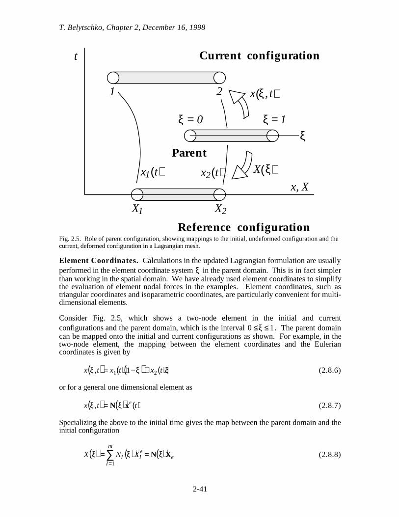
T. Belytschko, Chapter 2, December 16, 1998
Current configuration
Reference configuration
Parent
t
x, X
X1 X2
ξ = 0 ξ = 1
ξ
X ξ( )
x ξ, t( )1 2
x1 t( ) x2 t( )
Fig. 2.5. Role of parent configuration, showing mappings to the initial, undeformed configuration and thecurrent, deformed configuration in a Lagrangian mesh.
Element Coordinates. Calculations in the updated Lagrangian formulation are usuallyperformed in the element coordinate system ξ in the parent domain. This is in fact simplerthan working in the spatial domain. We have already used element coordinates to simplifythe evaluation of element nodal forces in the examples. Element coordinates, such astriangular coordinates and isoparametric coordinates, are particularly convenient for multi-dimensional elements.
Consider Fig. 2.5, which shows a two-node element in the initial and currentconfigurations and the parent domain, which is the interval 0 ≤ξ ≤ 1. The parent domaincan be mapped onto the initial and current configurations as shown. For example, in thetwo-node element, the mapping between the element coordinates and the Euleriancoordinates is given by
x ξ ,t( ) = x1 t( ) 1−ξ( )+ x2 t( )ξ (2.8.6)
or for a general one dimensional element as
x ξ ,t( ) = N ξ( )xe t( ) (2.8.7)
Specializing the above to the initial time gives the map between the parent domain and theinitial configuration
X ξ( ) = NII=1
m
∑ ξ( )XIe = N ξ( )Xe (2.8.8)
2-41

T. Belytschko, Chapter 2, December 16, 1998
which for the two-node element is
X ξ( ) = X1 1− ξ( ) + X2ξ (2.8.9)
The mapping between the Eulerian coordinates and the element coordinates, (2.8.6),changes with time, while the map between the initial configuration and the element domainis time invariant in a Lagrangian mesh. Therefore shape functions expressed in terms ofthe element coordinates by (2.8.8) will be independent of time. If the initial map is suchthat every point in the parent element ξ maps onto a unique point of the initialconfiguration, and for every point X there exists a point ξ , then the parent elementcoordinates can serve as material labels. Such a map is called one-to-one and onto. Themap between the parent domain and the current configuration must be one-to-one and ontofor all time; this is discussed further in Example 2.8.3 and Chapter 3.
As shown in Fig. 2.5, at any time the shape functions can be used to map between thecurrent and parent element configurations. Thus the element coordinates provide a linkbetween the initial configuration and the current configuration of the element which can beused in the evaluation of derivatives and integrals.
It follows from Eqs. (2.8.7) and (2.8.8) that the displacements can also be interpolatedby the same shape functions since
u ξ, t( ) = x ξ , t( ) − X ξ( ) = N ξ( ) xe t( ) − Xe( ) = N ξ( )ue t( ) (2.8.10)
The velocities and accelerations are also given by material derivatives of the displacement,while the test function is given by the same shape functions, so
v ξ ,t( ) = N ξ( )ve t( ) a ξ, t( ) = N ξ( ) u e t( ) δv ξ, t( ) = N ξ( )δve (2.8.11)
since the shape functions are independent of time.
Using Eqs. (2.8.2) and (2.6.5) and noting Eq.(2.8.3), the rate-of-deformation can beexpressed in terms of the shape functions by
Dx x, t( ) = v, x x ,t( ) = N , x X x, t( )( )ve t( ) (2.8.12)
where we have indicated the implicit dependence of the shape functions on the Euleriancoordinates. The rate-of deformation will be expressed in terms of nodal velocities via a Bmatrix by
Dx = v, x = Bve = BI
I=1
m
∑ vIe (2.8.13)
where
B = N ,x or BI = NI ,x (2.8.14)
2-42

T. Belytschko, Chapter 2, December 16, 1998
This B matrix differs from the B0 matrix used in the total Lagrangian formulation in thatthe derivatives are taken with respect to the Eulerian coordinates..
To compute the spatial derivative of the shape function, we use the chain rule
N,ξ = N , xx,ξ so N ,x = N,ξ x,ξ
−1 (2.8.15)
From the above, it follows that
Dx ξ, t( ) = x,ξ−1N,ξ ξ( )ve t( ) = B ξ( )ve t( ) B ξ( ) = N,ξ x ,ξ
−1 (2.8.16)
Internal and External Nodal Forces. We now use the procedure given in Sections2.4 and 2.5 to determine nodal forces corresponding to each term of the weak form on anelement level. The assembled equations and essential boundary conditions are developedsubsequently. The internal nodal forces will be developed from the virtual internal power.Defining the element internal nodal forces so that the scalar product with the virtualvelocities gives the internal virtual power, then from (2.7.6) and (2.8.13) we can write
δPe
int ≡ δveTfe
int = δv,xTσAdx
x1e t( )
x me t( )
∫ = δveT N, x
Tσ Adxx`
e t( )
x me t( )
∫ (2.8.17)
The transpose is taken of the first term in the integrand even though it is a scalar so that theexpression remains consistent when δv is replaced by a matrix product. From thearbitrariness of δve , it follows that
fei nt = N, x
T σAdxx 1
e t( )
xme t( )
∫ ≡ BTσAdxx1
e t( )
xme t( )
∫ or fein t = BT
Ω e t( )∫ σ dΩ (2.8.18)
We have explicitly indicated the time dependence of the limits of integration of the integralsto emphasize that the domain of integration varies with time. The internal nodal forces canthen be evaluated in terms of element coordinates by transforming (2.8.18) to the parentdomain and using the above with dx = x ,ξdξ , giving
fe
int = N ,xTσAdx = N,ξ
T x,ξ−1σAx,ξdξ =
ξ1
ξ m
∫x1
e t( )
xme t( )
∫ N,ξT σAdξ
ξ1
ξ m
∫ (2.8.19)
The last form in the above is nice, but this simplification can be made only in onedimension.
The external nodal forces are obtained from the expression for virtual external power(2.7.7):
δPeext = δve
Tfeext = δvTρbdΩ +
Ω te∫ δvT Atx( )
Γt
(2.8.20)
2-43

T. Belytschko, Chapter 2, December 16, 1998
Substituting (2.8.11) into the right hand side of the above and using the arbitrariness ofδve gives
feext = NTρbAdx +
x1e
xme
∫ NT At x( )Γt
e = NTρbdΩ+ Ω e t( )∫ NT Atx( )
Γte (2.8.21)
where the second term contributes only when the boundary coincides with a node of theelement.
Mass Matrix. The inertial nodal forces and mass matrix are obtained from the virtualinertial power (2.7.8):
δP inert =δveTfe
inert = δvTρDv
DtAdx
x1 t( )
xm t( )
∫ (2.8.22)
Substituting (2.8.11) into the above yields
feinert = ρNTNAdx
x1 t( )
xm t( )
∫ ˙ v e = Me˙ v e (2.8.23)
where the inertial force has been written as the product of a mass matrix M and the nodalaccelerations. The mass matrix is given by
Me = ρNTNA dxx1 t( )
x m t( )
∫ = ρNT N dΩΩ e t( )∫ (2.8.24)
The above form is inconvenient because it suggests that the mass matrix is a function oftime, since the limits of integration and the cross-sectional area are functions of time.However, if we use the mass conservation equation (2.2.10) in the form ρ0 A0dX =ρAdx ,we can obtain a time invariant form. Substituting the (2.2.10) into (2.8.24) gives
Me = ρ0NT NA0dXX1
Xm
∫ (2.8.25)
This formula for the mass matrix is identical to the expression developed for the totalLagrangian formulation, (2.4.11). The advantage of this expression is that it clearly showsthat the mass matrix in the updated Lagrangian formulation does not change with time andtherefore need not be recomputed during the simulation, which is not clear from (2.8.24).We will see shortly that any nodal force for a Lagrangian mesh can be computed by eitherthe total or updated Lagrangian formalism. The one which is chosen is purely a matter ofconvenience. Since it is more convenient and illuminating to evaluate the mass matrix inthe total Lagrangian form, this has been done.
Equivalence of Updated and Total Lagrangian Formulations. The internal andexternal nodal forces in the updated and total Lagrangian formulations can be shown to be
2-44
T. Belytschko, Chapter 2, December 16, 1998
identical. To show the identity for the nodal internal forces, we express the spatialderivative of the shape function in terms of the material derivative by the chain rule:
N, x X( ) = N, X
∂X∂x
= N, X F–1 = B0F–1 (2.8.26)
From the first equality we have N, xdx = N,XdX , and substituting this into (2.8.18) gives
feint = N ,x
T σAdx =x1 t( )
xm t( )
∫ N,XT σAdX
X1
Xm
∫ (2.8.27)
where the limits of integration in the third expression have been changed to the materialcoordinates of the nodes since the integral has been changed to the initial configuration. Ifwe now use the identity σA= PA0 , Eq.(2.2.9), we obtain from the above that
feint = N ,X
T PA0 dX X1
Xm
∫ (2.8.28)
This expression is identical to the expression for the internal nodal forces in the totalLagrangian formulation, (2.5.14). Thus the expressions for the internal nodal forces in theupdated and total Lagrangian formulations are simply two ways of expressing the samething.
The equivalence of the external nodal forces is shown by using the conservation ofmass equation, (2.2.10). Starting with (2.8.21) and using the (2.2.10) gives
feext = NT ρbAdx +
x1e
xme
∫ NT At x( )Γt
e= NT ρ0b A0dX +
X1
Xm
∫ NT A0t x0( )
Γte
(2.8.29)
where we have used the identity txA = tx0 A0 in the last term. The above is identical to
(2.4.8), the expression in the total Lagrangian formulation.
From this and the identity of the expression for the mass matrix, it can be seen that thetotal and updated Lagrangian formulations simply provide alternative expressions for thesame nodal force vectors. The formulation which is used is simply a matter ofconvenience. Moreover, it is permissible to use either of these formulations for differentnodal forces in the same calculation. For example, the internal nodal forces can beevaluated by an updated Lagrangian approach and the external nodal forces by a totalLagrangian approach in the same calculation. Thus the total and updated Lagrangianformalisms simply reflect different ways of describing the stress and strain measures anddifferent ways of evaluating derivatives and integrals. In this Chapter, we have also useddifferent dependent variables in the two formulations, the velocity and stress in the updatedformulations, the nominal stress and the displacement in the total formulation. However,this difference is not tied to the type of Lagrangian formulation, and we have done this onlyto illustrate how different independent variables can be used in formulating the continuummechanics problem. We could have used the displacements as the dependent variables inthe updated Lagrangian formulation just as well.
2-45

T. Belytschko, Chapter 2, December 16, 1998
Assembly, Boundary Conditions and Initial Conditions. The assembly ofthe element matrices to obtain the global equations is identical to the procedure describedfor the total Lagrangian formulation in Section 2.5. The operations of gather are used toobtain the nodal velocities of each element, from which the strain measure, in this case therate-of-deformation, can be computed in each element. The constitutive equation is thenused to evaluate the stresses, from which the nodal internal forces can be computed by(2.8.19). The internal and external nodal forces are assembled into the global arrays by thescatter operation. Similarly, the imposition of essential boundary conditions and initialconditions is identical and described in Section 2.4. The resulting global equations areidentical to (2.4.17) and (2.4.15). Initial conditions are now needed on the velocities andstresses. For an unstressed body at rest, the initial conditions are given by
vI = 0 , I = 1to nN σ I = 0, I =1 to nQ (2.8.30)
That initial conditions in terms of the stresses and velocities is more appropriate forengineering problems is discussed in Section 4.2. Nonzero initial values can be fit by anL2 projection described at the end of Section 2.4.
2-46

T. Belytschko, Chapter 2, December 16, 1998
Box 2.3 Updated Lagrangian Formulation
u( X, t ) = N X ξ( )( )ue t( ) = N I X ξ( )( )u Ie t( ) (B2.3.1)
.... v( X , t ) = N X ξ( )( )ve t( )= N I X ξ( )( )vIe t( ) (B2.3.2)
note N,x = N,ξ x,ξ−1
in each element
Dx =∂N I
∂xvI
e
I=1
m
∑ = Bve (B2.3.3)
evaluate s by constitutive equation
fe
i nt =∂N∂xΩ e
∫ σdΩ or fein t = BT
Ωe∫ σdΩ (B2.3.4)
feext = ρ
Ω e∫ NTbdΩ+ (NTAt x) Γ t
e (B2.3.5)
Me = ρ0Ωe∫ NTNdΩ same as total Lagrangian (B2.3.6)
M˙ u + f int = f ext (B2.3.7)
Example 2.8.1. Updated Lagrangian Form of Two-Node LinearDisplacement Element. This element is the same as in Example 2.5.1, Fig. 3, exceptthe updated Lagrangian treatment is now used. Recall that A0 and ρ0 are assumed to beconstant in each element. The velocity field is the same as for the updated Lagrangianelement, (2.5.19):
v X, t( ) = 1l0
X2– X , X – X1[ ]N X( )
1 2 4 4 4 3 4 4 4
v1 t( )v2 t( )
(2.8.31)
In terms of element coordinates, the velocity field is
2-47

T. Belytschko, Chapter 2, December 16, 1998
v ξ , t( ) = 1– ξ , ξ[ ]N ξ( )
1 2 4 3 4
v1 t( )v2 t( )
ξ =
X– X1l0
(2.8.32)
The displacement is the time integrals of the velocity, and sinceξ is independent of time
u ξ , t( ) = N ξ( )ue t( ) (2.8.33)
Therefore, since x = X + u
x ξ ,t( ) = N ξ( ) xe t( ) = 1– ξ ξ[ ] x1 t( )
x2 t( )
x,ξ = x2 − x1 = l (2.8.34)
where l is the current length of the element. For this element, we can express ξ in termsof the Eulerian coordinates by
ξ =
x– x1
x2 – x1=
x – x1
l , l = x2 – x1 , ξ, x =
1
l(2.8.35)
So ξ,x can be obtained directly, instead of through the inverse of x,ξ . This is not the casefor higher order elements.
The B matrix is obtained by the chain rule
B = N,x = N,ξ ξ,x = 1
l –1 , +1[ ] (2.8.36)
so the rate-of-deformation is given by
Dx = Bv e = 1
l v2– v1( ) (2.8.37)
Using (2.8.18) then gives
fe
int = BTσ Adx =x1
x2
∫ 1l
–1
+1
σ Adx
x1
x2
∫ (2.8.38)
If the integrand in (2.8.38) is constant, as if often is, then (2.8.38) yields
f e
int = Aσ–1
+1
(2.8.39)
Thus the internal nodal forces for the element correspond to the forces resulting from thestress σ. Note that the internal nodal forces are in equilibrium.
The external nodal forces are evaluated using (2.8.21)
2-48

T. Belytschko, Chapter 2, December 16, 1998
feext =
1– ξξ
x1
x2
∫ ρbAdx +1– ξ
ξ
Atx
Γ te
(2.8.40)
where the last term makes a contribution only if a node of the element is on the tractionboundary. Since x is a linear function of ξ and t, Eq. (2.8.16), b(x,t) can always beexpressed as a function of ξ and t. It is conventional to fit the data for b(x,t) by linearinterpolants for linear displacement elements (the information in higher order interpolationswill be beyond the resolution of the mesh). So we let
b ξ ,t( ) = b1 1−ξ( )+ b2ξ (2.8.41)
Substituting into (2.8.31) and integrating gives
f e
ext =ρAl6
2b1 + b2
b1 + 2b2
(2.8.42)
Comparison to Total Lagrangian. We will now compare the nodal forces to thoseobtained by the total Lagrangian formulation. Replacing σ in (2.8.39) by the nominalstress using Eq. (2.1.3a), we see that (2.8.39) and (2.5.27) are equivalent. It can easilybe shown that (2.8.29) and (2.8.21) lead to the same expression as (2.8.31).
To compare the external nodal forces, we note that by the conservation of matter, ρAl= ρ0 A0l0 . Using this in Eq. (2.8.42) gives (2.5.26), the total Lagrangian form of the nodalexternal forces. In the updated Lagrangian formulation, the mass from the total Lagrangianformulation is used, see Eq. (2.8.25), so the equivalence need not be considered.
Example 2.8.2. Updated Lagrangian of Three Node Element, QuadraticDisplacement Element The 3-node element is shown in Fig. 2.7. Node 2 can beplaced anywhere between the end-nodes, but we shall see there are restrictions on theplacement of this node if the one-to-one condition is to be met. We will also examine theeffects of mesh distortion.
t
X, xX1 X2 X3
x1(t) x2(t) x3(t)
x1 x2 x3
Fig. 2.7. Three node, quadratic displacement element in original and current configurations.
The displacement and velocity fields will be written in terms of the element coordinates
2-49

T. Belytschko, Chapter 2, December 16, 1998
u ξ, t( ) = N ξ( ) ue t( ) , v ξ , t( ) = N ξ( ) ve t( ) , x ξ ,t( ) = N ξ( ) xe t( ) (2.8.43)
where
N ξ( ) = 1
2 ξ2 –ξ( ) 1– ξ 2 12 ξ2 +ξ( )[ ] (2.8.44)
and
ueT = u1, u2 ,u3[ ] ve
T = v1 , v2 ,v3[ ] xeT = x1 , x2 , x3[ ] (2.8.45)
The B matrix is given by
B = N,x = x,ξ−1N,ξ (2.8.46)
= 12x,ξ
2ξ –1 – 4ξ 2ξ +1[ ] (2.8.47)
where
x,ξ = N,ξ xe = ξ– 12( ) x1– 2ξ x2 + ξ + 1
2( ) x3 (2.8.48)
The rate of deformation is given by
Dx = N,x ve = Bv e = 1
2x,ξ2ξ–1 – 4ξ 2ξ + 1[ ] ve (2.8.49)
This rate-of-deformation varies linearly in the element if x ,ξ is constant, which is the casewhen node 2 is midway between the other two nodes. However, when node 2 movesaway from the midpoint due to element distortion, x ,ξ becomes linear and the rate-of-deformation is a rational function. Furthermore, as node 2 moves from the center, itbecomes possible for x ,ξ to become negative or vanish. In that case, the mapping betweenthe current spatial coordinates and the element coordinates is no longer one-to-one.
The internal forces are given by (2.8.18):
fei nt = BTσ Adx =
x1
x3
∫ 1x,ξ
ξ – 12
–2ξξ + 1
2
σ Ax ,ξ dξ
–1
+1
∫ = σ A
ξ– 12
–2ξξ + 1
2
dξ
–1
+1
∫ (2.8.50)
where we have used dx = x , ξ dξ . Using (2.1.3), we can see that this expression isidentical to the internal force expression for the total Lagrangian formulation.
Mesh Distortion. We will now examine the effects of mesh distortion on this element.When x2 = 1
4 x3 + 3x1( ) , i.e. when node 2 of the element is one quarter of the element
length from node 1, then x,ξ = 12 x3– x1( ) ξ +1( ) , so x ,ξ = 0 at ξ =–1. Examining the
Jacobian given by Eq. (2.2.3)
2-50

T. Belytschko, Chapter 2, December 16, 1998
J =
A
A0x,X =
A
A0x,ξX,ξ
−1 (2.8.51)
we see that it will also vanish. By E. (2.2.4a) this implies that the current density becomesinfinite at that point. As node 2 moves closer to node 1, the Jacobian becomes negative inpart of the element, which implies a negative density and a violation of the one-to-onecondition. This corresponds to a violation of mass conservation and continuity of thedisplacement field. These situations are often masked by numerical quadrature, because thecondition must be more severe to appear at Gauss quadrature points.
The failure to meet the one-to-one condition can also affect the rate-of-deformation,which is given by Dx = Bve . From (2.8.37) we can see the potential for difficulties when
the denominator x ,ξ vanishes or becomes negative. When x2 = 14 x3 + x1( ), and x ,ξ =0 at ξ
=–1, then the rate-of-deformation becomes infinite at node 1. This property of quadraticdisplacement elements has been exploited in fracture mechanics to develop elements withsingular cracktip stresses called quarter-point elements, but in large displacement analysisthis phenomenon can be troublesome.
In one-dimensional elements the effects of mesh distortion are not as severe as inmulti-dimensional problems. In fact, the effects of mesh distortion can be alleviatedsomewhat in this element by using F as a measure of deformation, see Eq. (2.5.40). Thedeformation gradient F never becomes singular in the 3-node element if the initial positionof X2 is at the midpoint. However, any constitutive equation expressed in terms of F willdiffer markedly from one expressed in terms of the rate-of-deformation Dx when thestrains are large.
Example 2.8.3. Axisymmetric 2-Node Element. As an example where theconcept of the principle of virtual power or work becomes quite useful, we consider theanalysis of an axisymmetric two dimensional disc of constant thickness, a, which is thincompared to its dimensions so σ z = 0 . The only nonzero velocity is vr r( ) , which asshown, is only a function of the radial coordinate in an axisymmetric problem. Thenonzero Cauchy stresses and rate-of-deformations are written in cylindrical coordinatesusing Voigt notation
D =Dr
Dθ
σ =
σr
σθ
(2.8.52)
The rate-of-deformations are given by
Dr = vr ,r Dθ =vr
r(2.8.53)
and the momentum equation is
∂σ r
∂r+
σ r −σθ
r+ ρbr = ρ ˙ v r (2.8.54)
The boundary conditions are
2-51

T. Belytschko, Chapter 2, December 16, 1998
σ r a( ) = σa σ r b( ) =σ b (2.8.55)
rarb
ereθ
1 radiansegment
r
z
element
a
Fig. Schematic of axisymmetric discthe shaded area is considered in work terms
It is not necessary to integrate the momentum equation to obtain its weak form. By theprinciple of virtual power the weak form is
δ P = 0 ∀δvr ∈U0 (2.8.56)
The internal virtual power is obtained from the rate-of-deformation and stress
δPeint = δDrσr + δDθσθ( )ardr
r1e
r2e
∫ = δD T σ dΩΩe∫ (2.8.57)
where dΩ = ardr because a segment of one radian in the circumferential direction has beenchosen to avoid the factor 2π in all terms. The external virtual power is given by
δPeext = δvrρbrdΩ
Ω e∫ + art r( )Γt
(2.8.58)
where ar in the last term is the area of a one radian segment. The virtual inertial power isgiven by
δPe
inert = δvr ρ˙ v rdΩΩe
∫(2.8.59)
Consider a two-node finite element with a linear velocity field written in terms of elementcoordinates
v ξ ,t( ) = 1− ξ ξ[ ] v1 t( )
v2 t( )
(2.8.60)
2-52

T. Belytschko, Chapter 2, December 16, 1998
The rate-of-deformation is evaluated by Eq.() using the above velocity field andimmediately put into matrix form
D =Dr
Dθ
=− 1
r21
1r21
1− ξr
ξr
v1 t( )v2 t( )
= Bve (2.8.61)
The internal nodal forces are given by an expression identical to () except that the stress isreplaced by the column matrix
feint = BT σ dΩ
Ω e∫ =
− 1r21
1r21
1−ξr
ξr
σr
σθ
ardr
r1
r2
∫ (2.8.62)
The external nodal forces are given by
feext =
1−ξξ
r1
r2
∫ ρbrardr + art r( ) Γt(2.8.63)
The element mass matrix is given by
Me =1−ξ
ξ
r1
r2
∫ 1− ξ ξ[ ]ρardr
= ρar21
12
3r1 + r2 r1 + r2
r1 + r2 r1 +3r2
(2.8.64)
The lumped mass matrix can be computed by the row sum technique or by lumping half themass at each node, which gives, respectively
Me =ρar21
6
2r1 + r2 0
0 r1 + 2r2
row-sum
Me =ρar21 r1 + r2( )
4
1 0
0 1
lump
(2.8.65)
As can be seen the two lumping procedures give slightly different results.
2.9. Governing Equations for Eulerian Formulation
In an Eulerian formulation, the nodes are fixed in space and the independent variablesare functions of the Eulerian spatial coordinate x and the time t. The stress measure is theCauchy (physical) stress σ x , t( ) , the measure of deformation is the rate-of-deformation
Dx x ,t( ) . The motion will be described by the velocity v x, t( ) . In Eulerian formulations,the deformation is not expressed as a function of the reference coordinates since an
2-53

T. Belytschko, Chapter 2, December 16, 1998
undeformed, initial configuration cannot be established, and no counterpart of (2.2.1) isavailable.
Box. 2.4. Governing Equations for Eulerian Formulation
continuity equation (mass conservation):∂ρ∂t
+∂ ρv( )
∂x= 0 (B2.4.1)
momentum equation
ρA∂v
∂t+ v
∂v
∂x
=
∂ Aσ( )∂x
+ ρAb ρ∂v
∂t+ v
∂v
∂x
= ∂σ
∂x+ ρb (B2.4.2)
strain measure (rate-of-deformation): Dx = v,x (B2.4.3)
constitutive equation in rate form:
DσDt
=σ ,t x ,t( )+σ , x x, t( )v x ,t( ) = StσD Dx X , t ( ),σ X, t ( ),etc., t ≤ t( ) (B2.4.4)
energy conservation equationsame as before
The governing equations are summarized in Box 2.4. In comparison with the updatedLagrangian formulation we have just discussed, four points are noteworthy:
1. The mass conservation equation is now written as a partial differential equation;the form used with Lagrangian meshes is not applicable because it applies onlyto material points.
2. The material time derivative for the velocity in the momentum equation has beenwritten out in terms of the spatial time derivative and transport term.
3. The constitutive equation is expressed in rate form; the total form cannot be usedsince the stress and rate of deformation are functions of material coordinates in ahistory-dependent material.
4. The boundary conditions are now imposed on spatial points which do not movewith time.
The continuity equation has been written as a partial differential equation because it isnot possible to obtain an integral form such as Eq. (2.2.4) when the density is a function ofspatial coordinates. Therefore, the continuity equation must be treated as a separate partialdifferential equation, although there are approximations which enable the continuityequation to be omitted when the density changes little, as for a liquid or solid; these arediscussed in Chapter 7.
The constitutive equation needs to be expressed in terms of material coordinates forhistory-dependent materials, so it is treated in rate form in this formulation. It is thus aseparate partial differential equation.
In the general case, boundary conditions are required for the density, velocity andstress. As will be seen in Chapter 7, the boundary conditions for the density and stress inan Eulerian mesh depend on whether the material is flowing in or out at the boundary. Inthis introductory exposition, we consider only boundaries where there is no flow. Theboundary points are then Lagrangian, and the density and stress can be determined at thesepoints by the Lagrangian mass conservation equation, Eq. (2.2.10) and the constitutive
2-54

T. Belytschko, Chapter 2, December 16, 1998
equation, respectively. Therefore, there is no need for boundary conditions for thesevariables.
2.10 WEAK FORMS FOR EULERIAN MESH EQUATIONS
In the Eulerian formulation, we have 3 unknowns or dependent variables: the densityρ(x, t), the velocity v(x, t) and the stress σ(x, t). The rate-of-deformation can easily beeliminated from the momentum equations by substituting (B2.4.3) into the constitutiveequation (B2.4.4). Therefore, we will need three sets of discrete equations. A weak formsof the momentum equation, the mass conservation equation and the constitutive equationwill be developed. We will construct continuous solutions to the governing equations.The equations given in Box 2.4 can in fact have discontinuous solutions, withdiscontinuities in the density, stress and velocity, as when a shock occurs in the flow.However, we will take the approach of smearing any discontinuities over several elementswith a continuous function; this approach is called shock fitting or shock smearing. Thetrial and test functions will therefore be continuous functions of space.
We consider first the weak form of the continuity equation. The trial functions for thedensity are denoted by ρ x ,t( ) , the test functions by δρ x( ) The test functions and the trialfunctions for the continuity equation must be piecewise continuously differentiable, so
ρ x ,t( ) ∈R, R = ρ x ,t( ) ρ x ,t( ) ∈C0 x( ), ρ x, t( ) = ρ on Γρ (2.10.1)
δρ x( ) ∈R0 , R = δρ x( )δρ x( ) ∈C0 x( ), δρ xa( ) = 0, δρ xb( ) = 0 (2.10.2)
In this Section, we do not consider problems with prescribed densities on the boundaries.
The weak form of the continuity equation is obtained by multiplying it by the testfunction δρ x( ) and integrating over the domain. This gives
δρ( ρ ,t + ( ρv ) , x ) dx = 0
x a
x b
∫ ∀δρ ∈R 0 (2.10.3)
Only first derivatives with respect to the spatial variable of the density and velocity appearin the weak form, so there is no need for integration by parts. The consequence ofintegrating by parts are interesting and is examined in the Exercises.
The weak form of the constitutive equation is obtained the same way. We express thematerial derivative in terms of a spatial derivative and a transport term, giving
σ ,t + σ , xv− S( v, x ,etc ) = 0 (2.10.4)
The test and trial functions, δσ( x) and σ( x, t) , respectively, are subject to the samecontinuity and end conditions as for the density in the continuity equation, i.e., we letσ ∈ℜ , δσ ∈ℜ0 . The weak form of the constitutive equation is then obtained bymultiplying it by the test function and integrating over the domain:
δσ ( σ, t +σ ,xv −S( v, x ,etc )) dx = 0
xa
xb∫ ∀δσ ∈R 0 (2.10.5)
2-55

T. Belytschko, Chapter 2, December 16, 1998
As in the continuity equation, there is no benefit in integrating by parts. Neither this weakform nor the weak continuity equation have a clear physical meaning. They will be referredto as the weak continuity and constitutive equations.
The weak form of the momentum equation is obtained by integrating the test function
δv( x) over the spatial domain. The procedure is identical to that in the updated Lagrangianformulation in Section 2.7. The test and trial functions are defined by Eqs (2.7.1) and(2.7.2). The resulting weak form is
δv,x Aσ −δv ρAb − ρA
Dv
Dt
dx
x a
xb
∫ − δvAt x( )Γ t
= 0 (2.10.6)
or using (??)
δv,x Aσ +δvρA
∂v
∂t+v , xv − b
dx
x a
xb
∫ − δvAt x( )Γ t
= 0(2.10.7)
Note that the limits of the integration are fixed in space.
The weak form is identical to the principle of virtual power for the updated Lagrangianformulation except that the domain is fixed in space and the material time derivative isexpressed in its Eulerian form. Thus the weak form of the momentum equation can bewritten
δ P =δ P int− δ Pext +δ P inert = 0 ∀δv ∈U0 (2.10.8)
where
δP int = δv,xxa
xb
∫ σAdx = δDxxa
xb
∫ σAdx = δDxΩ∫ σΩ (2.10.9)
δP ext = δv
xa
xb
∫ ρbAdx + δvAt x( )Γ t
(2.10.10)
δ P inert = δvxa
xb
∫ ρ∂v
∂t+ v,xv
Adx
= δv
Ω∫ ρ
∂v
∂t+v, xv
dΩ (2.10.11)
All of the terms are identical to the corresponding terms in the principle of virtual power forthe updated Lagrangian formulation, except that the limits of integration are fixed in spaceand the material time derivative in the inertial virtual power has been expressed in terms ofthe spatial time derivative and the transport term. Similar expressions for the virtualpowers also hold on the element level.
2.11. FINITE ELEMENT EQUATIONS
2-56

T. Belytschko, Chapter 2, December 16, 1998
In a general Eulerian finite element formulation, approximations are needed for thepressure, stress and velocity. For each independent variable, test and trial functions areneeded. We will develop the equations for the entire mesh. For simplicity, we considerthe case where the segment is 0 ≤ x ≤ L. As mentioned before, we consider the case wherethe end points are fixed in space and the velocities on these points vanish. There are thenno boundary conditions on the density or stress and the boundary conditions on thevelocity are
v 0,t( ) = 0, v L, t( ) = 0 (2.11.1)
The mapping between spatial and element parent coordinates is given by
x = N I ξ( )x I (2.11.2)
In contrast to the Lagrangian formulations, this mapping is constant in time since the nodalcoordinates x I are not functions of time. The trial and test functions are given by
ρ x ,t( ) = NI
ρ x( )I =1
n N
∑ ρ I t( ) δρ x( ) = NIρ x( )
I=1
nN
∑ δρ I (2.11.3)
σ x, t( ) = NI
σ x( )I=1
nN
∑ σ I t( ) δσ x( ) = NIσ x( )
I=1
nN
∑ δσ I (2.11.4)
v x, t( ) = NI x( )
I= 2
nN −1
∑ vI t( ) δv x( ) = NI x( )I=2
nN −1
∑ δvI (2.11.5)
The velocity trial functions have been constructed so the velocity boundary condition isautomatically satisfied.
Substituting the test and trial functions for the density into the weak continuityequation gives
δρJ
J=1
nN
∑I=1
nN
∑ NJρNI
ρρI , t + NJρ ρv( ),x( )0
L
∫ dx = 0 (2.11.6)
Since this holds for arbitrary δρJ at interior nodes, we obtain
N I
ρNJρdxρJ ,t0
L
∫ + NIρ ( ρv ) ,x0
L
∫ dx = 0 I =1 to nN (2.11.7)
We define the following matrices
MIJ
ρ = NIρN J
ρdx0
L
∫ , Meρ = Nρ( )T
NρdxΩe∫ (2.11.8)
g I
ρ = NIρ ρv( ), x0
L
∫ dx , geρ = Nρ( )T
ρv( ), x0
L
∫ dx (2.11.9)
2-57

T. Belytschko, Chapter 2, December 16, 1998
The discrete continuity equation can be then be written as
MIJ
ρ ˙ ρ JJ
∑ + gIρ = 0 for I = 1 to nN , or Mρ ˙ ρ +gρ = 0 (2.11.10)
The matrices Mρ can be assembled from element matrices just like the mass matrix in themomentum equation. The column matrix gρ is obtained by a scatter, or vector assembly.
The matrix Mρ is time invariant and closely resembles the mass matrix. However, thecolumn matrix gρ varies with time and must be computed in every time step. In mostcases, the element matrices are integrated in the parent coordinate system.
The discrete form of the constitutive equation is obtained similarly. The result is
MIJ
σ ˙ ρ JJ
∑ + gIσ = hI
σ for I =1 to nN , or Mσ ˙ σ + gσ = h (2.11.11)
where
MIJσ = N I
σ NJσdx
0
L
∫ and Meσ = Nσ( )T
Nσ dΩΩe∫ (2.11.12)
g I
σ = NIσ vσ ,xdx
0
L
∫ and geσ = Nσ( )T
vσ ,xdΩΩ e∫ (2.11.13)
where the matrix relations on the right have been extracted from the indicial forms andimmediately specialized to elements by the procedure in Section 2.8.
Current
Original
t
x1 2
ξParent
x ξ( )
x ξ( )
Fig. 2.8 Eulerian element in current and original configurations, which are the same, and the mapping tothe parent element.
Momentum Equation. The weak form of the momentum equation is identical to theweak form for the updated Lagrangian formulation except for the inertial term. Thereforethe expressions for the internal and external nodal forces are identical. The inertial nodal
2-58

T. Belytschko, Chapter 2, December 16, 1998
forces for the Eulerian formulation are obtained in the following on an element level. Wedefine the inertial nodal forces by Eq. (2.7.8) which gives
δ Peiner = δve
Tfeinert = δve
T ρNΩe
∫T
N˙ v +v, xv( )Adx (2.11.14)
From the above, it follows that the inertial nodal forces are given by
feiner = Me
˙ v e + fetran (2.11.15)
where
Me = ρNΩ e
∫T
NAdx, fetran = ρv, xvAdx
Ωe
∫ (2.11.16)
The transport nodal forces have not been written in matrix form; they are quadratic in thenodal velocities. This term is needed in the Eulerian formulation because the nodes arefixed in space, so the time derivatives of the nodal velocities correspond to spatialderivatives. The mass matrix differs from the mass matrix in the Lagrangian meshes in thatit is a function of time: as the density in the element changes, the mass matrix will changecorrespondingly.
Example. Two-Node Eulerian Finite Element. The finite element equations aredeveloped for a one-dimensional, two node element with linear velocity, density and stressfields. The element, shown in Fig. 2.8, is of length l = x2 − x1 and unit cross-sectionalarea. As can be seen, the spatial configuration does not change with time since it is anEulerian element. The map between element and spatial coordinates is given by
x ξ( ) = 1− ξ ξ[ ] x1x2
e
≡ N ξ( )xe (2.11.17)
The density, velocity and stress are also interpolated by the same linear shape functions
ρ ξ( ) = N ξ( )ρe v ξ( ) = N ξ( )ve σ ξ( ) = N ξ( )σe (2.11.18)
Superscripts are not appended to the shape functions because all variables are interpolatedby the same shape functions.
Density Equation. The element matrices for the discrete continuity equation are given by
Me
ρ = NT Nx1
x2
∫ dx =1− ξ
ξ
0
1
∫ 1−ξ ξ[ ]ldξ =l6
2 1
1 2
(2.11.19)
ge
ρ = NT ρv( ),xx1
x2
∫ dx =1− ξ
ξ
0
1
∫ ρv( ),x l dξ (2.11.20)
2-59

T. Belytschko, Chapter 2, December 16, 1998
The geρ vector is usually evaluated by numerical quadrature. For linear interpolants it is
given by
g eρ =
1
6ρ2 − ρ1( ) 2v1 + v2
v1 + 2v2
+1
6v2 − v1( ) 2ρ1 + ρ2
ρ1 +2ρ2
(2.11.21)
The above matrix vanishes when the density and velocity are constant in the element.
Stress Equation. The element matrix for the stresses Meσ = Me
ρ . The vector g eσ is given
by
g eσ = NT vσ , x dx
x1
x2
∫ =1− ξ
ξ
0
1
∫ v1 1− ξ( ) +v2ξ( ) σ2 −σ1( ) dξ
= 16
σ 2 − σ1( ) 2v1 + v2
v1 +2v2
(2.11.22)
In summary, the finite element equations for the Eulerian formulation consists of threesets of discrete equations: the continuity equation, the constitutive equation, and themomentum equation, or equation of motion. The momentum equation is similar to theupdated Lagrangian form, except that the inertial term includes a transport term and varieswith time. All nodal forces are defined over fixed intervals in space. The semidiscreteforms of the continuity and constitutive equations are first order ordinary differentialequations. We have only developed the discrete equations for the case where the endpointsare fixed.
2.12 Solution Methods
We have seen so far that the momentum equation can be discretized with a Lagrangianmesh in the form
M˙ u = fext – f int = f (2.12.1)
These are ordinary differential equations in time.
In order to enable some nonlinear problems to be solved at this point, we now describethe simplest solution method, explicit time integration of the equations of motion for aLagrangian mesh. The most widely used explicit method is based on the central differenceformulas. Explicit integration can be simplified further by replacing M by a diagonal orlumped mass matrix.
We start at time t=0 using time steps ∆t , so that at time step n, t = n∆t . The value of
a function at n∆t is denoted by a superscript n, i.e., un ≡ u n∆t( ) . In the central difference
method, the velocities are approximated by
˙ u n = vn+1/2 = un+1/ 2 –un –1/ 2
∆ t = u(t +∆t/2)−u(t−∆t/ 2)∆ t (2.12.2)
2-60

T. Belytschko, Chapter 2, December 16, 1998
where the second equality is included to clarify the notation. Half time step values are usedfor the velocities. The accelerations are given by
˙ u n ≡ an = vn+1/2–vn–1/2
∆t (2.12.3)
In each case, the value of the derivative at the center of a time interval is obtained fromthe difference of the function values at the ends of the interval, hence the name centraldifference formulas. The flow chart for an explicit program is then given by the followingBox.
Box 2.5 Flowchart for Explicit Time Integration of Lagrangian Mesh
1. Initial conditions and initialization: set v0 , σ0 ; n = 0 , t = 0; compute M
2. get f n
3. compute accelerations an = M−1f n
4. update nodal velocities: vn+1
2 = vn+ 12
−α + α∆tan : α =12 if n = 0
1 if n > 0
5. enforce essential boundary conditions: if node I on Γv : vIn = v xI , tn( )
6. update nodal displacements: un +1 = un +∆tvn+12
7. update counter and time: n ← n +1, t ← t +∆ t8. output, if simulation not complete, go to 2
Module: get f1. GATHER element nodal displacements ue
n and velocities ven+1/ 2
2. compute measure of deformation
3. compute stress by constitutive equation σen
4. compute internal nodal forces by equation in Box.
5. compute external nodal forces on element and fe = feext − fe
int
5. SCATTER element nodal displacements to global matrices
Updating for the displacements by Eq. (6) then does not require any solution ofalgebraic equations. Thus, in a sense, explicit integration is simpler than static linear stressanalysis. As can be seen from the flowchart, most of the explicit program is astraightforward interpretation of the governing equations and the time integration formulas.The program begins with the enforcement of the initial conditions; procedures for fittingdifferent initial conditions have already been described. The first time step is somewhatdifferent from the others because only a half-step is taken. This enables the program tocorrectly account for the initial conditions on the stresses and velocities.
Most of the programming and computation time is in computing the element nodalforces, particularly the internal nodal forces. The nodal forces are computed element-by-element. Prior to starting the element computations, the element nodal velocities anddisplacements are gathered from the global arrays. As can be seen from the flowchart, thecomputation of the internal nodal forces involves the application of the equations which areleft in strong form, the strain equation and the constitutive equation, followed by theevaluation of the internal nodal forces from the stress, which emanates from the weak form
2-61

T. Belytschko, Chapter 2, December 16, 1998
of the momentum equation. When the computation of the element nodal forces iscompleted, they are scattered to the global array according to their node numbers.
The essential boundary conditions are enforced quite easily as shown. By setting thenodal velocities equal to the prescribed nodal velocities at all nodes on prescribed velocityboundaries, the correct displacements result, since the velocities are subsequently integratedin time. The placement of this step in the flowchart insures that the correct velocities areavailable in the nodal force computation. The initial velocities must be compatible with theboundary conditions; this is not checked in this flowchart but would be checked in aproduction program. The reaction forces can be obtained by outputting the total nodalforces at the prescribed velocity nodes.
It can be seen from the flowchart that the traction boundary conditions enter onlythrough the external nodal forces. Therefore, for a traction-free boundary, nothing need bedone: the homogeneous traction boundary condition is enforced naturally in a weak senseby the finite element solution. However, the traction boundary condition is only satisfiedapproximately.
Stability Criterion. The disadvantage of explicit integration is that the time step mustbe below a critical value or the solution "blows up" due to a numerical instability. This isdescribed in detail in Chapter 6. Here we limit ourselves to pointing out that the criticaltime step for the 2-node elements described in this Chapter is given by
∆ tcrit = l
c (2.12.4)
where l is the current length of the element and c is the wave speed given by
c2 = Eση / ρ (2.12.5)
where Eση is the modulus in the elastic relation between Cauchy stress and rate-of-
deformation. For nonlinear materials, Eση is replaced by the current tangent modulus
EσD
t = ˙ σ Dx
(2.12.6)
A computer program for the explicit integration of the one-dimensional updated andtotal Lagrangian formulation is given in Appendix B.
Appendix A. Derivation of Conservation Equations in 1D.
In this Appendix, simple derivations of the conservation equations in one dimensionwill be given. These are "engineering" derivations which develop these equations insimplest terms, and they lack the mathematical rigor and generality associated with thederivations found in texts on continuum mechanics.
We first derive the equation of conservation of mass, also called the continuityequation. Consider a segment of the rod shown in Fig. 2.7, which in the initial, orundeformed, state is of length ∆X, cross-sectional area A0 and density ρ0. In the deformedstate this Lagrangian segment has length ∆x, area A and density ρ. The subdomain is amaterial, or Lagrangian subdomain, in that all material points remain in the subdomain and
2-62

T. Belytschko, Chapter 2, December 16, 1998
the right and left end points are the same material points. No flow of material occurs in orout of the segment. Therefore, by mass conservation, the mass in the undeformed segmentmust equal the mass of the deformed segment:
ρA∆x = ρ0 A0∆X (A.1)
currentconfiguration
referenceconfiguration
∆x
∆xAρb
t
x, X
Ao P( ) X+∆XAo P( ) X
∆X
Aσ( ) x Aσ( ) x+ ∆x
∆XAo ρob
Fig. 2.9. A segment of a rod in the reference (initial, undeformed) and current configurations showing allforces acting on the segment.
Dividing by ∆X and taking the limit as ∆X → 0 gives
ρ0 A0 = ρA ∂x∂X
= ρAF or ρ0 X( )A0 X( ) = ρ X ,t( )A X ,t( )F X ,t( ) (A.2)
The above is one form of the equation of mass conservation. On the right hand side theindependent variables have been indicated to stress that this equation only holds whenexpressed in terms of the material coordinates; the variables on the RHS are functions oftime, whereas the variables on the LHS are independent of time.
To obtain another form of this equation, we note that the volumes of the segment arerelated by the Jacobian by dΩ = JdΩ0 . Since dΩ = Adx and dΩ0 = A0dX , it follows that
J = AA0
F (A.3)
Substituting the above into (A.1) gives the another form of the mass conservation equation
2-63
T. Belytschko, Chapter 2, December 16, 1998
ρ0 X( ) = ρ X ,t( ) J X, t( ) (A.4)
The above equation also applies in multi-dimensional problems.
Momentum Equation. The momentum equation is derived by considering the segmentof the rod shown in Fig. 2.9. The forces on the deformed segment are shown in Fig. 2.9and consist of the forces arising from the stress, which act on the right and left hand end ofthe segment, and the body force; the body force is distributed over the entire segment andits net resultant is placed at the center of the segment. On the left hand end of the segmentthe force is Aσ( )
x, i.e. the product of the stress and the current area at the point x . The
force due to the stress on the right hand end is given by Aσ( )x+∆x
. The resultant force due
to the body force is obtained by multiplying b x + ∆x2( ) by the mass of the segment ρA∆x .
So if we write Newton's second law for the segment we have
–Aσ x + Aσ( )
x+∆x+ ρAb( )
x+ ∆x2
∆x = ρA˙ u ( )x+ ∆x
2∆x (A.5)
where the LHS is the sum of the resultant forces from the stress and the body force and theRHS is the product of the mass of the segment and its acceleration.
The forces due to the stresses are now expanded by a Taylor's series about themidpoint of the segment, with the product Aσ treated as a single function, which gives
Aσ( )
x+∆x= Aσ( )
x+∆x / 2 +∂ Aσ( )
∂x x+∆x / 2
∆x
2+O ∆x 2( ) (A.6a)
Aσ( ) x = Aσ( ) x+∆x / 2 − ∂ Aσ( )
∂x x+∆x / 2
∆x2
+ O ∆x2( ) (A.6b)
The use of a Taylor series expansion of course presupposes that the function is smoothenough so that the first derivative exists; this is not the case wherever the stress or the areais discontinuous. Substituting (A.6) into (A.5) and dividing by ∆x gives
Aσ( ),x + ρAb = ρA˙ u (A.7)
The above is the momentum equation for a one-dimensional continuum of varying cross-section.
To derive the momentum equation in the reference configuration, we note that theforces on the sides of the segment are given by multiplying the nominal stress by the initialarea, A0P . The net force due to the body force is ρ0 A0b∆X since ρ0b is a force per unitinitial volume and the initial volume is A0∆X . The mass of the segment is ρ0 A0∆X .Writing Newton's second law for the segment gives
–A0P( )
X+ A0P( )
X +∆X+ ρ0 A0b( )
X+ ∆X2
∆X = ρ0 A0b˙ u ( )X+ ∆X
2∆X (A.8)
2-64

T. Belytschko, Chapter 2, December 16, 1998
where the LHS is the sum of all forces acting on the segment and the RHS is the mass timethe acceleration. Expressing the forces due to the nominal stresses by a Taylor series as in(A.6), but in terms of the material coordinate X , substituting into (A.8) and dividing by∆X gives the momentum equation in Lagrangian form
A0P( ) ,X + ρ0A0b = ρ0A0 u (A.9)
The above can easily be transformed to the Eulerian form, Eq. (A.7). By the stresstransformation (2.1.2), we have A0P = Aσ , so
A0P( ) ,x = Aσ( ),x = Aσ( ),x x,X = Aσ( ),x F (A.10)
where the chain rule has been used in the third step, followed by the definition of F in Eq.(2.2.2). Substituting the (A.10) into (A.9) gives
0 = Aσ( ),x F + ρ0 A0b − ρ0A0˙ u = Aσ( ),x F + FρAb − FρA˙ u
where the continuity equation (A.2) has been used in the last step. Dividing by F thengives the momentum equation in Eulerian form. Note that the body force in the Lagrangianand Eulerian momentum equations is identical. Some authors distinguish the body force inthe total form by a subscript naught, i.e., Malvern (1969, p. 224), but this is superfluous ifthe body force is considered a force per unit mass so that ρb is a force per unit volume.
SUMMARY
The finite element equations have been developed for one-dimensional continua ofvarying cross-section. Two mesh descriptions have been used:
1. Lagrangian meshes, where the nodes and elements move with the material;2. Eulerian meshes, in which nodes and elements are fixed in space.
Two formulations have been developed for Lagrangian meshes:1. a total Lagrangian formulation, in which the strong form is expressed in spatial
coordinates, i.e. the Eulerian coordinates;2. an updated Lagrangian formulation, where the strong form is expressed in the
material, i.e. the Lagrangian coordinates.
In both cases, the element formulation is most conveniently executed in terms of theelement coordinates. The mapping of the element coordinates from current and originalconfiguration for a valid finite element discretization is one-to-one and onto. Furthermore,the mapping to the original configuration is time invariant, so the element coordinates canserve as surrogate material coordinates.
It has also been shown that the updated and total Lagrangian formulations are tworepresentations of the same mechanical behavior, and each can be transformed to the otherat both the level of partial differential equations and the level of the discrete finite elementequations. Thus the internal and external forces obtained by the total Lagrangianformulations are identical to those obtained by the updated formulation, and the choice offormulation is purely a matter of convenience.
2-65

T. Belytschko, Chapter 2, December 16, 1998
The equation of motion corresponds to the momentum equation and is obtained fromits weak form. As has been illustrated in the case of explicit time integration, the otherequations, measure of deformation and constitutive, are used in the course of computingthe internal nodal forces to update the displacements. The weak form and discreteequations have been structured so that their relationship to the corresponding terms in thepartial differential equation of momentum conservation is readily apparent: the internalforces correspond to the stress terms, and the internal work (or power); the external forcescorrespond to the body forces and external work (or power); the terms Ma correspond tothe inertial terms (d'Alembert) forces and the inertial work (or power). Thiscorrespondence is summarized in Fig. 8, which shows the steps which are used to convertthe partial differential equation of momentum balance to a set of ordinary differentialequations which are called the equations of motion. This process is called a spatialdiscretization or semidiscretization.
The discretization has been carried out for the general case when inertial forces are notnegligible. If the inertial forces can be neglected, the term Ma is omitted from the discreteequations. The resulting equations are either nonlinear algebraic equations or ordinarydifferential equations, depending on the character of the constitutive equation.
The governing equations have been developed for a one-dimensional rod of varyingcross-section and from these a weak form has been developed by integrating over thedomain. When the equations are given in terms of partial derivatives with respect to thematerial derivatives, it is natural to develop the weak form by integrating over theundeformed domain. This leads to the total Lagrangian formulation where all nodalforces are obtained by integrating over the material coordinates. When the partialderivatives are with respect to the spatial coordinates, it is natural to integrate over thecurrent configuration, which leads to the updated Lagrangian formulation .
The process of discretization for multidimensional problems is very similar.However, in multi-dimensional problems we will have to deal with the major consequenceof geometric nonlinearities, large rotations, which are completely absent in one-dimensionalproblems.
Exercises
Exercise: Repeat Example 2.8.3 for spherical symmetry, where
h =η r
ηθ
ηφ
s =
σ r
σθ
σφ
give B , feint , fe
ext , Me
2-66