chapter 2: handling large data sets in r and linuxyee/784/files/ksrub.pdf · 2.2 linux/unix toolsy...

Chapter 2: Handling Large Data Sets in R and Linux

© Thomas Yee

Statistics Department, Auckland University

July 2018

[email protected]

http://www.stat.auckland.ac.nz/~yee

© Thomas Yee (Stat Dept, UoA) Chapter 2. Large Data Sets in R and Linux 1/93July 2018 1 / 93

http://www.stat.auckland.ac.nz/~yee

Chapter Outline

Chapter Outline1 2.1 Introduction

Why Use Linux/Unix?

2 2.2 Linux/Unix tools†AWKSEDCompressionOther Linux/Unix Tools

3 2.3 Getting data into RGetting Data into R

4 2.4 R memory etc.Block linear models

5 2.5 Sorting

6 2.6 Merging data†7 2.7 R programming

Using Less Time and Memory in STricks in R and SPLUS

© Thomas Yee (Stat Dept, UoA) Chapter 2. Large Data Sets in R and Linux 2/932018 2 / 93

Chapter Outline

Writing good codeExercise

8 2.8 RecursionExerciseExercises

9 2.9 Relational Databases†

10 2.10 Calling FORTRAN and C from R†

11 2.11 Miscellaneous NotesLessons

12 2.12 References†

© Thomas Yee (Stat Dept, UoA) Chapter 2. Large Data Sets in R and Linux 3/932018 3 / 93

2.1 Introduction

2.1 Introduction

This chapter is to present some ideas about using R more efficiently withina data mining context. In these situations greater efficiency can make abig difference. Most people know how to get R to give an answer,butgetting the right answer efficiently is the main topic of this chapter.However, since R is run on a computer, we need to look at things a bitmore holistically than just R itself.

R is not really suitable for data mining where the data sets are really big.Nevertheless, there are some things to be aware of and avoided in order tomake life easier when dealing with a large data set. Even if your data setisn’t huge, the things in this chapter will help you use R more efficiently.

We’ll also look at some Linux/Unix tools that can be helpful with big datasets. They can do certain things easily, e.g., editing a huge text file withan ordinary editor may not be possible because it is too large to hold in

Chapter 2. Large Data Sets in R and Linux 4 / 93

2.1 Introduction

memory at once. We’ll look at “sed” and “awk”, but other alternatives arePERL and Python.

The real problem is that programmers have spent far too much time worrying about

efficiency in the wrong places and at the wrong times; premature optimization is the

root of all evil (or at least most of it) in programming. (D. Knuth)


2.1 Introduction

Nb. The most comprehensive source of information are the R Manuals,either online or in book form. You need to use them all the time.

A fundamental difference between R and S-PLUS is that R holds allvariables and data in memory, whereas S-PLUS writes them to disk. Bothhave their advantages and disadvantages.

Sections daggered (†) are non-examinable, as well as any quote at the bottom of the

page.


2.1 Introduction Why Use Linux/Unix?

Why Use Linux/Unix?

This chapter applies particularly to R (in the past I also consideredS-PLUS). In general, it is important to know the strengths and weaknessesof the tools you use.

Nb. Linux/Unix tools are available for Windows—seehttp://www.cygwin.com. There is also something called Lindoze.

It is efficient, stable, multi-tasking, mature, full of tools, and has beenused in scientific computing for many years.


http://www.cygwin.com

2.2 Linux/Unix tools†

2.2 Linux/Unix Tools†

The Linux/Unix philosophy is that everything is a small tool, and to get ajob done, one uses several of these tools to do it. Hence the idea of anapplication such as xemacs, an editor which can do almost everything, isactually foreign. [Nb. emacs is not an editor, but a religion, a way of life.]

To find information about a Linux/Unix command type man <command>.Of course, the downside is that you need to remember the commandname! There are many books on Linux/Unix and its applications.Furthermore, there are lots of resources on the internet.

Asking if computers can think is like asking if submarines can swim. (Edwin Dykstra)


2.2 Linux/Unix tools† AWK

AWK

Awk is a pattern scanning and processing language. It is available on allLinux/Unix systems. A full description can be found in Aho, Kernighanand Weinberger (1988).

The best way to start learning awk is to look at a few examples. Here aresome.

“I gather, young man, that you wish to be a member of parliament. The first lesson that

you must learn is: when I call for statistics about the rate of infant mortality, what I

want is proof that fewer babies died when I was prime minister than when anyone else

was prime minister. That is a political statistic.” (Winston Churchill)



AWK Example 1

Suppose there is a text file bispp.prob which is

1.751695e+02 -4.190860e+01 8.439016e-01

1.752298e+02 -4.190740e+01 8.444533e-01

1.752900e+02 -4.190630e+01 8.407476e-01

1.753502e+02 -4.190510e+01 8.389687e-01

1.754105e+02 -4.190380e+01 8.357652e-01

1.754707e+02 -4.190260e+01 8.336947e-01

1.755309e+02 -4.190130e+01 8.302924e-01

If we used a text editor to create a file called f.awk:

{ print $3 " " $2 }

then if we type awk -f f.awk bispp.prob then we would get



8.439016e-01 -4.190860e+01

8.444533e-01 -4.190740e+01

8.407476e-01 -4.190630e+01

8.389687e-01 -4.190510e+01

8.357652e-01 -4.190380e+01

8.336947e-01 -4.190260e+01

8.302924e-01 -4.190130e+01



AWK Example 2

Suppose there is a text file nametag.txt which is

Smith Mary A Corinth

Ting Hua-Sieng D Philippi

Bong Fredd H Ephesus

Mok Ching-Ching P Ephesus

We want to use LATEX to produce nametags for these people. The columnsare, respectively, surname, first name, NZ university (A=Auckland,H=Hamilton etc.), overseas city where they come from.

Suppose we use a text editor to create a file called f.awk:



{

print $2 " " $1 " \\\\";

if($3 == "A") center = "Auckland";

if($3 == "H") center = "Hamilton";

if($3 == "P") center = "Palmerston North";

if($3 == "W") center = "Wellington";

if($3 == "C") center = "Christchurch";

if($3 == "D") center = "Dunedin";

print center " \\\\";

print "\\vspace{5mm}";

print "";

}

Then if we type

awk -f f.awk nametag.txt > outthen the file out will be



Mary Smith \\

Auckland \\

\vspace{5mm}

Hua-Sieng Ting \\

Dunedin \\

\vspace{5mm}

Fredd Bong \\

Hamilton \\

\vspace{5mm}

Ching-Ching Mok \\

Palmerston North \\

\vspace{5mm}

which can be pasted into a LATEX file.



AWK Example 3

Suppose there is a text file data3.txt which is

3 1 4 1 5

9 2 6 5 3

6 1 2 3 4

5 6 7 8 9

Suppose f3.awk is:

# This program outputs certain variables

# and a cross-product term

{

x2 = $2;

x5 = $5;

if (!($1 < 4 && $2 < 5)) print $1 " " \

$3 " " x2 " " x5 " " x2*x5;

}



Then if we type awk -f f3.awk data3.txt the output will be

9 6 2 3 6

6 2 1 4 4

5 7 6 9 54

Note one has to have a back-slash as the last character on a line in orderto have the next line as a continuation line.


2.2 Linux/Unix tools† SED

SED

Available on all Linux/Unix systems is “Sed”, a stream editor. A streameditor is used to perform basic text transformations on an input stream (afile or input from a pipeline). While in some ways similar to an editorwhich permits scripted edits (such as ed), sed works by making only onepass over the input(s), and is consequently more efficient. But it is sed’sability to filter text in a pipeline which particularly distinguishes it fromother types of editors. Another advantage is that one doesn’t have to havethe entire file in memory at once.

Notes for the following example

1 “s” stands for substitute.

2 There are tabs in the file.



SED Example 1

Suppose the text file f1.sed:

s/ A / Auckland /

s/ H / Hamilton /

s/ P / Palmerston North /

s/ D / Dunedin /

s/ C / Christchurch /

s/ W / Wellington /

s/Corinth//

s/Ephesus//

s/Philippi//

then if we type sed -f f1.sed nametag.txt then we would get

Smith Mary Auckland

Ting Hua-Sieng Dunedin

Bong Fredd Hamilton

Mok Ching-Ching Palmerston North



SED Example 2

Suppose the text file f2.sed:

s/e/ee/

s/o/oo/g

and the file f2.sed:

the quick brown fox jumped

over the lazy dog.

Then if we type sed -f f2.sed d2.txt then we would get

thee quick broown foox jumped

ooveer the lazy doog.

Note: “g” stands for global, i.e., it substitutes all of them in the file. Thedefault is to replace the first occurrence on each line.


2.2 Linux/Unix tools† Compression

Compression

The standard Linux/Unix commands compress and uncompress

compress and uncompress files. There are better ones around, e.g., GNU’sgzip and gunzip, bzip2 and bunzip2.

There is a command for storing all the files in a directory as a singlecompressed file. It is, e.g., zip -r fname.zip directory, which storesthe whole directory directory in the file fname.zip, and in compressedform. The command unzip fname.zip will restore it back.

Another way of doing what zip does is to store the directory as a file, andthen to compress this file. The first step can be done using the tar (tapearchive) command. For example, tar cvf tar.fname directories

creates the file tar.fname out of directories (and tar xvf

tar.fname restores it back into a directory). Then gzip tar.fname

could be used to compress the tar file.

See gzfile() by typing ?gzfile.Chapter 2. Large Data Sets in R and Linux 20 / 93

2.2 Linux/Unix tools† Other Linux/Unix Tools

Other Linux/Unix Tools

The commands wc, sort, cmp, grep, diff, plus many others, are usefulin general. For example,

aitken% wc *

5 16 316 awk.aux

29 107 6208 awk.dvi

158 671 6011 awk.log

360 953 7097 awk.tex

6 18 102 emp.data

10 42 180 f3.awk

6 25 94 interest.awk

1 3 12 interest.dat

498 759 5827 nametag.tex

6 24 217 nametag.txt

40 62 452 out

1119 2680 26516 total


2.3 Getting data into R


Almost always, the data comes from some “outside” application orprocess, and must be read into R. Reading data into a statistical systemfor analysis and exporting the results to some other system for reportwriting can be frustrating tasks that can take far more time than thestatistical analysis itself.

In general, statistical systems like R are not particularly well suited tomanipulations of large-scale data. Some other systems are better than Rat this. Rather than duplicating functionality in R we can make the othersystem do the work! (For example, Therneau & Grambsch (2000)comment that they prefer to do data manipulation in SAS and then usesurvival5 in S-PLUS for the analysis.)



scan()

scan() is one of the most basic ways to read data in. Interactively andwithout arguments, it reads from the keyboard until an empty lineterminates the input. One can read a 2 column file of numbers by, e.g.,

> args(scan)

function (file = "", what = double(), nmax = -1L, n = -1L, sep = "",

quote = if (identical(sep, "\n")) "" else "'\"", dec = ".",

skip = 0L, nlines = 0L, na.strings = "NA", flush = FALSE,

fill = FALSE, strip.white = FALSE, quiet = FALSE, blank.lines.skip = TRUE,

multi.line = TRUE, comment.char = "", allowEscapes = FALSE,

fileEncoding = "", encoding = "unknown", text, skipNul = FALSE)

NULL

> xy <- scan("xyData", list(x = numeric(), y = character()))

then xy$x and xy$y contain the 2 columns. See the other arguments toscan(). The 2 arguments nmax and n can increase efficiency.



read.table() and write.table()

The functions read.table() and write.table() are probably the mostsimplest methods to read in and write out a nice data frame in textformat. A common useful option is header = TRUE/FALSE.

Note that read.table() is slower than scan(). Its performance cansubstantially be improved by using the colClasses argument to specifythe classes to be assumed for the columns of the table. Andread.table() and scan() can read files that have been compressedusing any of several compression algorithms.

Note that there are variants of read.table(), e.g., read.csv() andread.delim(), which differ only in the defaults.



The file() Function

Suppose foo.dat contains two columns of numbers, and we want tocompute the sums of each column. Then

aa <- file("foo.dat", "r")

sumcol <- rep(0, 2)

repeat {z <- scan(aa, what=list(x=0, y=0), n=1000)

if (!length(z$x)) break

sumcol[1] <- sumcol[1] + sum(z$x)

sumcol[2] <- sumcol[2] + sum(z$y)

}close(aa)

print(sumcol)



will read the file a bit (500 rows) at a time and do what we want.

This is an example of a ‘connection’. Connections are an unappreciatedresource of S4, and not very well documented. For further informationread the chapter in Chambers (1998) several times.

Exercise Write a small awk program to do the above.


2.3 Getting data into R Getting Data into R

Getting Data into R

See the file R-data.pdf.

The function count.fields() is useful and is like NF in Awk.

Other ideas: data.table has fread() which is supposed to be faster thanread.csv(), and a data.table is an enhanced data.frame. In fact, adata.table inherits from data.frame, and is supposed to be fast andmemory-efficient. It is worth studying well, and there is a homepagehttp://r-datatable.com for this contribution.


http://r-datatable.com


Note:

> version

_

platform x86_64-pc-linux-gnu

arch x86_64

os linux-gnu

system x86_64, linux-gnu

status

major 3

minor 5.0

year 2018

month 04

day 23

svn rev 74626

language R

version.string R version 3.5.0 (2018-04-23)

nickname Joy in Playing



Exporting Data Between Packages

Very often data has to be put into another form so that another packagecan read it in. Sometimes text format is used for this because it can beviewed and printed easily.

R can import data from several other statistical packages using the foreignpackage. Currently, this works for Minitab, S, S-PLUS, SAS, SPSS andStata. See the manual “R Data Import/Export” (that comes with thedistribution) for details. An alternative is haven, which has the same goalas foreign but it can read binary SAS7BDAT files and Stata13 files, andalways returns a data frame.

To export a S object one way is to use dump(), e.g., dump("u", "u.q")

which creates the file u.q which can be source()’d.

In Hmisc there is sas.get().


2.4 R memory etc.

2.4 R memory etc.

As R holds everything in memory it is important to know a little abouthow to control for its size and how the internals of R handles computermemory.

There are two things to consider:

1 the hardware. The computer chip(s) may be 32-bit but are usually64-bit. They are usually have a multi-core processor. The amount ofphysical computer memory, and the amount of virtual memory.

2 the software. In particular, the compiler from which R is built.

A diplomat is a man who always remembers a woman’s birthday but never remembers

her age. (Robert Frost)


2.4 R memory etc.

Here are some miscellaneous notes.

1 R 3.5.0 (released in 2018) had “Arithmetic sequences created by 1:n,seq along, and the like now use compact internal representations viathe ALTREP framework.”

2 R 3.0.0 (released in 2013) had “the inclusion of long vectors(containing more than 231 − 1 elements!). R now has 64 bit supporton all platforms, support for parallel processing, Matrix, and . . . ”

3 http://adv-r.had.co.nz/memory.html conveys some issuesrelating to memory in R.

4 The files R-admin.pdf, R-ints.pdf and R-intro.pdf give detailsabout memory including how to build R with certain memory limits.On a 64-bit machine one can choose between a 32-bit build and a64-bit build. The file R-data.pdf talks about relational databases.

5 Some relevant functions or things to investigate:

?Memory


http://adv-r.had.co.nz/memory.html

2.4 R memory etc.

memory.size()

memory.limit()

gc(). Objects of fixed size are stored in cons cells (e.g., 28 bytes each),variable sized objects are stored in a heap of Vcells (e.g., 8 bytes each).object.size(), e.g.,

> object.size(runif(1e6))

8000048 bytes

> print(object.size(runif(1e6)), units = "MB")

7.6 Mb

6 Install via --max-mem-size.

7 See http://www.matthewckeller.com/html/memory.html.


http://www.matthewckeller.com/html/memory.html

2.4 R memory etc.

Parallel computing

This is a quickly changing and important field. It seems computer chipsare not getting as fast as one would like, therefore PCs these days comewith more of them.

Packages foreach and doParallel provide ways of writing parallel code thatwill run on all systems, without having to worry about details of parallelcomputation on each platform. See also package multicore.


2.4 R memory etc. Block linear models

Block linear models

S-PLUS has a function lmBlock() which fits a linear model in blocks. Itruns like as follows.

> lmBlock(y ~ x + z, block.dh)

Iteration #:1, Total rows processed = 10000










[,1]

(Intercept) 0.002834771

x 0.699796077

z -0.001169790



In R there are the biglm, bigmemory, ff, filehash, R.huge, spam, sparseMand speedglm packages. Others packages include SOAR and track.

Note: an ordinary call to lm() to fit a linear model y = Xβ + ε createsabout 7 copies of the model matrix X; this is wasteful!

Recall that β̂ = (XTWX)−1XTWy for a LM.

Here is an example from the online help.



> library("biglm"); data("trees", package = "datasets")

Loading required package: DBI

> dim(trees)

[1] 31 3

> ff <- log(Volume)~log(Girth)+log(Height)

> chunk1 <- trees[1:10, ]

> chunk2 <- trees[11:20, ]

> chunk3 <- trees[21:31, ]

> a <- biglm(ff, chunk1)

> a <- update(a, chunk2)

> a <- update(a, chunk3)

> coef(a)

(Intercept) log(Girth) log(Height)

-6.6316 1.9826 1.1171



Block Multiplication

If we partition matrices A and B as follows, then(A11 A12

A21 A22

)(B11 B12

B21 B22

)=

(A11B11 + A12B21 A11B12 + A12B22

A21B11 + A22B21 A21B12 + A22B22

).

In classical regression theory, W = diag(w1, . . . ,wn) and X is the n × pdesign/model matrix. Then the theory behind this is that

XTWX =n∑

i=1wix ixT

i and XTWy =n∑

i=1wiyix i . The index i can be

broken into B blocks, i.e., X = (XT1 , . . . ,X

TB )T so that

XTWX =B∑

b=1

XTb WbXb etc.



A limitation of this method is that data-dependent terms are not allowedin the formula (e.g., see the biglm online help). For example, the functionsmin(), max(), mean(), sd(), var(), bs(), ns(), poly(), scale() willcause incorrect Xb block matrices to be constructed. For further details,see smart prediction in Yee (2015).

Exercise Run the following code snippet and explain why things havegone wrong.

n <- 20 # Create some data first

set.seed(86) # For reproducibility of the random numbers

ldata <- data.frame(x2 = sort(runif(n)), y = sort(runif(n)))

library("splines") # To get ns() in R

fit1 <- lm(y ~ ns(scale(x2), df = 5), data = ldata)

plot(y ~ x2, ldata, main = "Safe prediction fails")

lines(fitted(fit1) ~ x2, data = ldata)

new.ldata <- data.frame(x2 = sort(runif(n)))

points(predict(fit1, new.ldata) ~ x2, new.ldata,

type = "b", col = 2, err = -1)



Then run the following code snippet and explain why things are correct.

library("VGAM")

fit2 <- vglm(y ~ sm.ns(sm.scale(x2), df = 5), uninormal, data = ldata)

# [email protected]

plot(y ~ x2, ldata, main = "Smart prediction")

lines(fitted(fit2) ~ x2, data = ldata)

points(predict(fit2, new.ldata, type = "response") ~ x2, new.ldata,

type = "b", col = 2, err = -1)


2.5 Sorting

2.5 Sorting

Sorting observations is a significant task in data mining. Sometimes it is agood idea to sort the data first (by one particular variable).

Classically, the fastest (internal) sorting algorithms are O(n log n), e.g.,quicksort. However, if all the data cannot be held in memory at once, thenone has an external sorting problem. There have been efficient algorithmsof this type that have been developed.

Exercise: Suppose n is large. Show that the cost of quicksorting a 2nsized problem is more than twice the cost of the n sized problem.


2.5 Sorting

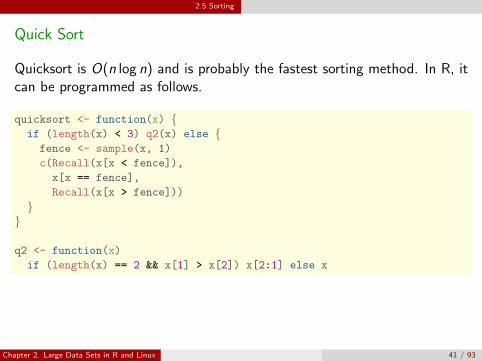
Quick Sort

Quicksort is O(n log n) and is probably the fastest sorting method. In R, itcan be programmed as follows.

quicksort <- function(x) {if (length(x) < 3) q2(x) else {fence <- sample(x, 1)

c(Recall(x[x < fence]),

x[x == fence],

Recall(x[x > fence]))

}}

q2 <- function(x)

if (length(x) == 2 && x[1] > x[2]) x[2:1] else x


2.5 Sorting

Sorting by Variables

If X is a matrix then two methods for sorting the rows by the first column is

> X[sort.list(X[, 1]), ]

> ooo <- order(X[, 1])

> X[ooo, ]

Sorting the data is needed when using lines(), e.g.,

par(mar = c(5, 4, 0.1, 0.1), mfrow = c(1, 2))

set.seed(784)

n <- 10; x <- runif(n); y <- x^2

plot(x, y, type = "n"); lines(x, y)

ooo <- order(x)

plot(x, y); lines(x[ooo], y[ooo])

This gives the following figure.


2.5 Sorting

0.2 0.4 0.6 0.8

0.0

0.2

0.4

0.6

0.8

x

y

●

●

●

●

●

●

●

●

●

●

0.2 0.4 0.6 0.8

0.0

0.2

0.4

0.6

0.8

xy


2.6 Merging data†

2.6 Merging Data†

Merging data sets is a common task. SAS is good at that, and offersseveral types of merging—concatenation, match-merging, updating etc.Concatenation in S can be achieved by careful use of rbind() andcbind().

Note: there is also the reshape package which can be an enormoustimesaver and an incredibly useful tool. For example, melt() and cast()

provide the ability to “aggregate” or tabulate a dataset.Merging Example


2.6 Merging data†

> one <- data.frame(x = 1:3, y = 2:4, z = 3:5)

> two <- data.frame(y = c(1:3, 7), z = c(2:4, 8),

w = c(3:5, 9), t = c(4:6, 10))

> one

x y z

1 1 2 3

2 2 3 4

3 3 4 5

> two

y z w t

1 1 2 3 4

2 2 3 4 5

3 3 4 5 6

4 7 8 9 10

> merge(one, two)

y z x w t

1 2 3 1 4 5

2 3 4 2 5 6


2.6 Merging data†

> merge(one, two, all = TRUE)

y z x w t

1 1 2 NA 3 4

2 2 3 1 4 5

3 3 4 2 5 6

4 4 5 3 NA NA

5 7 8 NA 9 10

> merge(one, two, by = "y")

y x z.x z.y w t

1 2 1 3 3 4 5

2 3 2 4 4 5 6


2.6 Merging data†

> merge(one, two, by = "y", all = TRUE)

y x z.x z.y w t

1 1 NA NA 2 3 4

2 2 1 3 3 4 5

3 3 2 4 4 5 6

4 4 3 5 NA NA NA

5 7 NA NA 8 9 10

> args(merge)

function (x, y, ...)

NULL

For merging huge files with limited memory, try joining them usingPostgreSQL (aka Postgres) and then hauling it back into R.


2.7 R programming

2.7 R Programming

Programming well in S requires a lot of learning. Advanced books includeChambers (1998), Chambers (2008) and Venables and Ripley (2000).More modern treatments include Wickham (2015a) and Wickham (2015b).A somewhat outdated book, but simpler to read, is Becker et al. (1988).

Like all languages, R has its weak points, and good programmers knowthem all and how to get around those problems. We will try to focus onproblems that occur especially because of large data sets.

To write portable code it is useful to make use of .Machine, whichcontains machine dependent constants.


2.7 R programming

> unlist(.Machine) # This is on a 64-bit machine

double.eps double.neg.eps double.xmin

2.2204e-16 1.1102e-16 2.2251e-308

double.xmax double.base double.digits

1.7977e+308 2.0000e+00 5.3000e+01

double.rounding double.guard double.ulp.digits

5.0000e+00 0.0000e+00 -5.2000e+01

double.neg.ulp.digits double.exponent double.min.exp

-5.3000e+01 1.1000e+01 -1.0220e+03

double.max.exp integer.max sizeof.long

1.0240e+03 2.1475e+09 8.0000e+00

sizeof.longlong sizeof.longdouble sizeof.pointer

8.0000e+00 1.6000e+01 8.0000e+00

For example, .Machine$double.eps is the smallest value of 2x (where xis integer), such that 1 + .Machine$double.eps > 1.


2.7 R programming Using Less Time and Memory in S

Using Less Time and Memory in S

It is well-known that S is (relatively) slow on looping, and that for ()

loops are less efficient in S than vectorized expressions. And you shouldwrite functions which minimize the required number of copies of large datasets, e.g., avoid growing.

Chambers (1998) recommends keeping things simple. In organizing data,S deals best with a fairly small number of pieces rather than a deeplynested organisation of structures within structures.

In R all data is stored in RAM. There is no disk swapping in (core) R yetbut some work has been done in this area.



Time and Memory in S

Time and memory, when used as measures of the efficiency of a function,can have many meanings. The time required by a function might be anyof the following:

1 CPU time: the time the computer spends actively processing thefunction.

2 Elapsed time: the time elapsed on a clock, stopwatch, or othertime-keeping device. Generally, you are most interested in elapsedtime, but unfortunately, elapsed time is not a particularly reliablemeasure of efficiency because it can vary widely from one executionto the next. Disk activity and other processes running can affect theelapsed time.



3 Programmer time: the time it takes the programmer to write andmaintain a function. Often, “computationally efficient” functions takemuch longer to write than simpler alternatives. If the function will beused infrequently then it may not be worth the extra effort.

R is a ratty, old, cobbled-together piece of crap (compared with what we now know is

possible). (Ross Ihaka, 2012-08)



Main memory , or RAM: physical memory built into the computer andaccessible from the CPU during processing.

Virtual memory : when a program uses more memory than available RAMthen data not actively being processed is swapped to a hard disk, freeingup RAM. A portion of the hard disk must generally be committed tosupporting swap operations; this is called the swap space. Virtual memoryallows much larger programs to be run, but incurs an extra time cost. Harddisks are significantly slower than RAM, as each swap involves disk I/O.



Virtual Memory†

When temporary variables are needed, using the same name can avoidwastage. For example, consider the following function:

g <- function(n = 125000) {tmp <- runif(n)

tmp1 <- 2 * tmp

tmp2 <- trunc(tmp1)

mean(tmp2 > 0.5)

}

This requires 4.5 million bytes to complete, while the following slightlymodified version needs only 2.5 million:



g1 <- function(n = 125000) {tmp <- runif(n)

tmp <- 2 * tmp

tmp <- trunc(tmp)

mean(tmp > 0.5)

}

(The 0.5 million byte chunks come from the logical vectors such as tmp >

0.5 and is.na(x) in the call to mean().)



Measuring Time

system.time() is useful for measuring the speed of executed code in R.

> args(system.time)

function (expr, gcFirst = TRUE)

NULL

Here is an example extracting a column from a matrix.

> bigdf <- data.frame(x1 = runif(100000)) # Big 1-coln data frame

> system.time(for (i in 1:5000) avec <- bigdf[, 1]) # Slow

user system elapsed

0.024 0.004 0.026

> system.time(for (i in 1:5000) adf <- bigdf) # Faster

user system elapsed

0.004 0.000 0.002



Now the three values returned are the user, system and elapsed times, inseconds. The user time is the time spent running user code. The systemtime is the time spent in system calls (e.g., reading and writing files). Theelapsed time is the actual time it took for the expression to be evaluated;this is usually the most important one.


2.7 R programming Tricks in R and SPLUS

Tricks in R and S-PLUS

If you use R to analyse a big data set you can use some tricks andadvanced features to help you handle big data sets. Here are a few ideas.

1 object.size() tells how big an object is (in bytes).In R, there is the gc() function; also type R --help for other options.

2 Some objects can be made smaller (but have possibly lessfunctionality), e.g.,

> fit <- lm(y ~ x1 + x2 + x3, x = FALSE, y = FALSE, qr = FALSE)



From Chambers (1998)

Pages 167–175 of Chambers (1998) discusses methods in the S4 languageto handle big data sets. Here are some of his advice.

Use whole-object computations—they act on an object, or a major pieceof an object, in one step. That is, the basic hint is to do computations andthe objects they return in whole-object terms. For example,

for (i in 1:length(w))

if (w[i] > 0) y[i] <- y[i] * w[i] else

y[i] <- y[i] / (1 - w[i])

is perfectly legal but will be slow if the objects are large. One does betterby



> pos <- w > 0; neg <- !pos

> y[pos] <- y[pos] * w[pos]

> y[neg] <- y[neg] / (1- w[neg])

which is called vectorization. An alternative is to use

> y <- y * ifelse(w > 0, w, 1/(1-w))


2.7 R programming Writing good code

Writing good code

Writing good code requires careful planning and discipline. Here are somehints to use when programming in S.

(i) Use Vectorized Arithmetic

S is set up to operate on whole vectors quickly and efficiently. If possible,you should always set up your calculations to act on whole vectors orsubsets of whole vectors, rather than looping over individual elements.Your principal tools should be subscripts and built-in vectorized functions.For example, suppose you have a set x of 30 observations collected overtime, and you want to calculate a weighted average, with the weights givensimply by the observation index. This is a straightforward calculation in S:

> wt.ave <- sum(x*1:30)/sum(1:30)



Because you may want to repeat this calculation often on data sets ofvarying lengths, you can easily write it as a function:

wt.ave <- function(x) {wt <- seq(along = x)

sum(x*wt)/sum(wt)

}

Here we created weights for each element of x simply by creating aweights vector having the same length as x. S performs its mathematicsvectorially, so the proper factor is automatically matched to theappropriate element of x. (Note: use weighted.mean()).

Even if you only want to calculate with a portion of the data, you shouldstill think in terms of the data object, rather than the elements that makeit up. For example, in diving competitions, there are usually six judges,each of whom assigns a score to each dive. To compute the diver’s score,



the highest and lowest scores are thrown out, and the remaining scores aresummed and multiplied by the degree of difficulty:

diving.score <- function(scores, difficulty=1) {scores <- sort(scores)[-c(1, length(scores))]

sum(scores) * difficulty

}

We use sort() to order the scores, then use a negative subscript to returnall the scores except the highest and lowest.

By now, these examples should be obvious. Yet seeing that these areindeed obvious solutions is a crucial step in becoming proficient atvectorized arithmetic. Less obvious, but of major importance, is to uselogical subscripts instead of for loops and if statements. For example,here is a straightforward function for replacing elements of a vector thatfall below a certain user-specified threshold with 0:



Over.thresh <- function(x, threshold) {for (i in 1:length(x))

if (x[i] < threshold)

x[i] <- 0

x

}

The “vectorized” way to write this uses ifelse():

Over.thresh2 <- function(x, threshold)

ifelse(x < threshold, 0, x)

But probably the fastest, most efficient way is to simply use a logicalsubscript:

Over.thresh3 <- function(x, threshold) {x[x < threshold] <- 0

x

}



(This is essentially what ifelse() does, except that ifelse() includesprotection against NA’s in the data. If your data have no missing values,you can safely use logical subscripts.)



(ii) Avoid for Loops

In S, follow the rule:

Avoid for, while, and repeat loops.

This applies to elements within a data structure in general.

It is not always possible to avoid loops in S. Two common situations inwhich loops are required are the following:

1 Operations on individual elements of a list. The apply() family(lapply(), mapply(), rapply(), sapply(), tapply(), vapply(),etc.) is recommended for this purpose. Note there is a fallacy thatapply() is always faster than for ().



2 Operations on vectors that contain dependencies, so that result[i]depends on result[i-1]. For example, cummax() calculates thecumulative maximum vector, so that

> cummax(c(1, 3, 2, 4, 7, 5, 6, 9))

[1] 1 3 3 4 7 7 7 9

The ith term cannot be calculated until the (i − 1)-th term is known. Inthese situations, loops are unavoidable. When you must use loops,following a few rules will greatly improve the efficiency of your functions:

1 Avoid growing a data set within a loop in S. Always create a data setof the desired size before entering the loop; this greatly improves thememory allocation. If you don’t know the exact size, overestimate itand then shorten the vector at the end of the loop.

2 In S-PLUS avoid looping over a named data set. If necessary, saveany names and then remove them by assigning NULL to them,perform the loop, then reassign the names.



(iii) Avoid Growing Data Sets

Avoid “growing” atomic data sets, either in loops or in recursive functioncalls in S.

For example, consider:

> grow <- function() {x <- NULL

for (i in 1:1e4)

x <- rbind(x, i:(i+9))

x

}> system.time(grow())

user system elapsed

0.444 0.028 0.475



The “no grow” version allocates memory for the full 1000 element matrixat the beginning:

> no.grow <- function() {x <- matrix(0, nrow = 1e4, ncol = 10)

for (i in 1:1e4)

x[i, ] <- i:(i+9)

x

}> system.time(no.grow())

user system elapsed

0.008 0.000 0.007

The detrimental effect of growing data sets will become very pronouncedas the size of the data object increases.



Here’s another example. Suppose we want to keep the results in a vectorres. Do not use

res <- NULL

for (iter in 1:1000)

res <- c(res, myfunction(iter, moreargs))

as this forces a copy of res to be made at each iteration; rather use

res <- numeric(1000)

for (iter in 1:1000)

res[iter] <- myfunction(iter, moreargs)

This is even more important if the result is a matrix rather than a vector.In some circumstances the final size of res may be unknown, in whichcase allocate a sufficient size and shrink the vector at the end of the loop.



(iv) Reuse Computations

For example, consider the following fragment:

> y <- log(x)

> z <- y + 1

Here y is used only once, but creates an object as large as the original x.It is better to replace the two line fragments above with the followingsingle line:

> z <- log(x) + 1



(v) Reuse Code

The efficiency of a piece of software needs to be measured not only by thememory it uses and the speed with which it executes, but also by the timeand effort required to develop and maintain the code. One important wayyou can simplify development and maintenance is to reuse code, bypackaging frequently used combinations of expressions into new functions.

Object-oriented programming (OOP) methods are a way of reusing code.

Simplicity, simplicity, simplicity! I say, let your affairs be as two or three, not a hundred

or a thousand. Simplify, simplify. (H. D. Thoreau, Walden)



(vi) Avoid Recursion

One common programming technique is even more inefficient in S-PLUSthan looping—it is recursion. Recursion is memory inefficient because eachrecursive call generates a new frame, with new data, and all these framesmust be maintained by S-PLUS until a return value is obtained.

In R recursion is not particularly expensive unless a modification of avariable is performed within the function. More generally, R makes copiesof the argument of a function when it is modified or assigned a value. Thisis a part of lazy evaluation.

For example, our original Fibonacci sequence function used recursion:



> fib <- function(n) {old.opts <- options(expressions = 512 + 512 * sqrt(n))

on.exit(options(old.opts))

fibiter <- function(a, b, count) {if (count == 0) b else

Recall(a + b, a, count-1)

}fibiter(1, 0, n)

}>

> system.time(fib(177))

user system elapsed

0 0 0

QuestionWhy is Recall() used?SolutionIf the function is renamed it will still work.



It can be more efficiently coded as a while loop:

> fib.loop <- function(n) {a <- 1

b <- 0

while (n > 0) {temp <- a

a <- a + b

b <- temp

n <- n - 1

}b

}>

> system.time(fib(177))

user system elapsed

0.004 0.000 0.004



(v) Use Specialized Functions

R has quite a number of specialized functions to do common operationsmore efficiently than simple programming. Here are some simple examples.

1 colSums() (not apply(, 2, sum)), .colSums(),

2 rowSums(), .rowSums(),

3 colMeans(), .colMeans(),

4 rowMeans() (not apply(, 1, mean)), .rowMeans(),

5 crossprod(), etc.

Sometimes it makes little difference, but sometimes it makes a bigdifference.At a more higher level, sometimes special structure in a statistical modelcan be exploited, e.g., GLAM for generalized linear array models seeglamlasso().


2.7 R programming Exercise

Exercise

The following code accumulates 1000 samples (with replacement) from afinite population. How could be made to run faster?

mat <- matrix(0, 1000, 6)

for (i in 1:1000)

mat[i, ] <- sample(x, 6, replace = TRUE)

SolutionChoose one sample of size 6000 and place it directly in a matrix:mat <- matrix(sample(x, 6000, replace = TRUE), 1000, 6)

but this is only possible for sampling with replacement, of course.

Not all calculations can be vectorized, especially those that depend on theresult of the previous calculation. The functions cumsum(), cumprod(),cummax() and cummin() are sometimes useful to vectorize calculations ofthis sort.


2.8 Recursion

2.8 Recursion

This is a small detour into recursion, which is a subject area worthknowing something about.

A function that calls itself is said to be recursive. Many definitions can bedefined elegantly in a recursive way. For example,n! = n × (n − 1)× · · · × 2× 1, 0! ≡ 1 defines the factorial of n, son! = n × (n − 1)!.

myfactorial <- function(i) {if (length(i)!=1 || round(i) != i || i < 0)

stop("argument 'i' is not a non-negative integer")

# integer overflow

# storage.mode(i) <- "double"

i <- i * 1.0

if (i == 0) 1.0 else i * myfactorial(i - 1.0)

}


2.8 Recursion

Useful functions: do.call() and Recall().

Several puzzles can be solved by recursion. For example, the Towers ofHanoi, and the Baguenaudier—a centuries old puzzle consisting ofinterlaced rings and a looped double rod which one wants to remove.


2.8 Recursion Exercise

Exercise

The Fibonacci series {1, 1, 2, 3, 5, 8, 13, . . .} is well known in mathematics.It starts with the numbers 1 and 1, and then successively adds the last twonumbers of the series to get the next one. Use this algorithm to do thefollowing.

1 Write a small R program to return the nth Fibonacci number. It alsohas an argument called all which, if set TRUE, returns the vector ofall the first n elements in the series.

Your function should do the following.


2.8 Recursion Exercise

> args(fibonacci)

function (n, all = FALSE)

NULL

> fibonacci(45)

[1] 1134903170

> fibonacci(45, all = TRUE)

[1] 1 1 2 3 5 8

[7] 13 21 34 55 89 144

[13] 233 377 610 987 1597 2584

[19] 4181 6765 10946 17711 28657 46368

[25] 75025 121393 196418 317811 514229 832040

[31] 1346269 2178309 3524578 5702887 9227465 14930352

[37] 24157817 39088169 63245986 102334155 165580141 267914296

[43] 433494437 701408733 1134903170

2 Repeat the above, but write another version that uses C orFORTRAN.

3 What is the smallest value of n for which overflow occurs?


2.8 Recursion Exercises

Exercises

1 The Hofstadter function is defined as

G (n) =

{0, n = 0;n − G (G (n − 1)), n ≥ 1.

Write an R program to compute the Hofstadter function. Compute itsvalues for n = 1, 2, . . . , 13.


2.8 Recursion Exercises

2 The Ackermann function is a two parameter function of x and y ,both natural numbers, with a third parameter n (also a naturalnumber) that controls the complexity. It is defined as

A(0, x , y) = x + 1,

A(n, x , 0) =

x , n = 1;0, n = 2;1, n = 3;2, n ≥ 4;

A(n, x , y) = A(n − 1,A(n, x , y − 1), x)

if n > 0 & y > 0.

Write an R program to compute the Ackermann function.Difficult: prove that A(1, x , y) = x + y , A(2, x , y) = xy ,A(3, x , y) = xy . Can you obtain an expression for A(4, x , y)?

Which reminds me: fortran does not allow recursion!


2.9 Relational Databases†

2.9 Relational Databases†

R was designed to interface with other software, e.g., Hadoop and Spark.Along these lines, something which is only mentioned here, but is to beemphasized, is that relational databases are a recommended place to dothe computations and then the results are transferred into R. An exampleof a relational database is MySQL, which happens to be the world’s mostpopular open source database. See the course STATS 220 for moreinformation.

Around 2012 Oracle released Oracle R Enterprise.

The file R-data.pdf talks about relational databases.


2.10 Calling FORTRAN and C from R†


With large data sets one can save time and memory by calling a compiledlanguage from within R/S-PLUS. This is a powerful feature. Thelanguages supported are FORTRAN and C (and C++). Why theselanguages? Because both R and S-PLUS are written in C. BothFORTRAN and C are similar in terms of the way they store numericalnumbers, hence they both can be supported.

Some relevant functions include

.Fortran()

> args(.Fortran)

function (.NAME, ..., NAOK = FALSE, DUP = TRUE, PACKAGE, ENCODING)

NULL



.C()

> args(.C)

function (.NAME, ..., NAOK = FALSE, DUP = TRUE, PACKAGE, ENCODING)

NULL

.Call()

> args(.Call)

function (.NAME, ..., PACKAGE)

NULL

Package Rcpp is becoming very popular these days. . .


2.11 Miscellaneous Notes

2.11 Miscellaneous Notes

data.table seems to be a popular way to get better efficiencycompared to data.frame().

The following projects/packages/commercial tools can help R handlebig data sets: RevoScaleR, Foreach for parallel programming, renjin,FastR, pqR for a pretty quick R interpreter.

Both REvolution and Netezza are heavily into parallel processing andlarge datasets. REvolution released several Rpackages (foreach,iterators and doMC) that address parallel processing.

The bigdata package makes it possible to replace R’s commoncreation of multiple copies of a dataset that can be represented as amatrix, by a single copy that is held on disk and accessed via pointers.All of part of the data can then be brought into physical memory, asrequired for processing. The ff package makes it possible, with somelimitations, to store data frames in this way.


2.11 Miscellaneous Notes Lessons

Lessons

The following comes from Ross Ihaka’s 782 notes.

Optimizing R performance is a very dark art indeed.

Knowing about the detail of how functions work internally can behelpful but is not essential.Experimentation with the code and timing the results withsystem.time() can reduce run times by orders of magnitude.

In general, vectorisation is a big win and converting loops intovectorised alternatives almost always pays off.

Code profiling can give a way to locate those parts of a programwhich will benefit most from optimization.



Profiling

Profiling is a useful tool which can be used to find out how much time isbeing spent inside each function when some R code is run.

When profiling is turned on, R gathers information on where the programis at regularly spaced time points (20 millisecond separation by default)and stores the information in a file.

After profiling is turned off the information stored in the file can beanalysed to produce a summary of how much time is spent in eachfunction.

It can be quite surprising to find out just where R is spending its time andthis can help to find ways to make programs run faster.



The following profiling example will enable us to find out where R isspending its time.

> Rprof()

> for (ii in 1:100)

sortx <- sort(runif(1e5))

> Rprof(NULL)

> prof <- summaryRprof()

> prof$by.self

self.time self.pct total.time total.pct

"order" 0.60 90.91 0.60 90.91

"runif" 0.06 9.09 0.06 9.09


2.12 References†

2.12 References†

Aho, A. V., Kernighan, B. W., Weinberger, P. J., 1988. The AWKProgramming Language. Addison-Wesley Pub. Co., Reading, MA,USA.

Baumer, B. S., Kaplan, D. T., Horton, N. J., 2017. Modern DataScience with R. Chapman and Hall/CRC, Boca Raton, FL, USA.

Becker, R. A., Chambers, J. M., Wilks, A. R., 1988. The New SLanguage: A Programming Environment for Data Analysis andGraphics. Wadsworth & Brooks/Cole, Pacific Grove, CA, USA.

Braun, W. J., Murdoch, D. J., 2008. A First Course in StatisticalProgramming with R. Cambridge University Press, Cambridge, UK.

Chambers, J. M., 1998. Programming with Data: A Guide to the SLanguage. Springer, New York, USA.


2.12 References†

Chambers, J. M., 2008. Software for Data Analysis: Programmingwith R. Statistics and Computing. Springer, New York, USA.

Chambers, J. M., 2016. Extending R. The R Series. Chapman &Hall/CRC, New York, USA.

Chambers, J. M., Hastie, T. J. (Eds.), 1993. Statistical Models in S.Chapman & Hall, New York, USA.

de Vries, A., Meys, J., 2012. R for Dummies. Wiley, Chichester, WestSussex.

Manoochehri, M., 2014. Data Just Right: Introduction to Large-scaleData & Analytics. Addison-Wesley, Upper Saddle River, NJ, USA.

Therneau, T. M., Grambsch, P. M., 2000. Modeling Survival Data:Extending the Cox Model. Springer, New York, USA.

Venables, W. N., Ripley, B. D., 2000. S Programming.Springer-Verlag, New York, USA.


2.12 References†

Venables, W. N., Ripley, B. D., 2002. Modern Applied Statistics WithS, 4th Edition. Springer-Verlag, New York, USA.

Wickham, H., 2015a. Advanced R. Chapman & Hall/CRC, BocaRaton, FL, USA.

Wickham, H., 2015b. R Packages: Organize, Test, Document andShare Your Code, 1st Edition. O’Reilly Media, Sebastopol, CA, USA.

Yee, T. W., 2015. Vector Generalized Linear and Additive Models:With an Implementation in R. Springer, New York, USA.


chapter 2: handling large data sets in r and linuxyee/784/files/ksrub.pdf · 2.2 linux/unix toolsy...

Documents