chapter 2 fourier analysis of signals - audiolabs-erlangen.de · 2016-01-15 · chapter 2 fourier...

Chapter 2Fourier Analysis of Signals

As we have seen in the last chapter, music signals are generally complex sound

mixtures that consist of a multitude of different sound components. Because of this

complexity, the extraction of musically relevant information from a waveform con-

stitutes a difficult problem. A first step in better understanding a given signal is to

decompose it into building blocks that are more accessible for the subsequent pro-

cessing steps. In the case that these building blocks consist of sinusoidal functions,

such a process is also called Fourier analysis. Sinusoidal functions are special in

the sense that they possess an explicit physical meaning in terms of frequency. As

a consequence, the resulting decomposition unfolds the frequency spectrum of the

signal—similar to a prism that can be used to break light up into its constituent

spectral colors. The Fourier transform converts a signal that depends on time into

a representation that depends on frequency. Being one of the most important tools

in signal processing, we will encounter the Fourier transform in a variety of music

processing tasks.

In Section 2.1, we introduce the main ideas of the Fourier transform and sum-

marize the most important facts that are needed for understanding the subsequent

chapters of the book. Furthermore, we introduce the required mathematical notions.

A good understanding of Section 2.1 is essential for the various music processing

tasks to be discussed. In Section 2.2 to Section 2.5, we cover the Fourier transform

in greater mathematical depth. The reader who is mainly interested in the music

processing applications may skip these more technical sections on a first reading.

In Section 2.2, we take a closer look at signals and discuss their properties from

a more abstract perspective. In particular, we consider two classes of signals: ana-

log signals that give us the right physical interpretation and digital signals that

are needed for actual digital processing by computers. The different signal classes

lead to different versions of the Fourier transform, which we introduce with math-

� Springer International Publishing Switzerland 2015M. Müller, Fundamentals of Music Processing,DOI 10.1007/978-3-319-21945-5_2

39

40 2 Fourier Analysis of Signals

ematical rigor along with intuitive explanations and numerous illustrating exam-

ples (Section 2.3). In particular, we explain how the different versions are interre-

lated and how they can be approximated by means of the discrete Fourier transform

(DFT). The DFT can be computed efficiently by means of the fast Fourier transform

(FFT), which will be discussed in Section 2.4. Finally, we introduce the short-time

Fourier transform (STFT), which is a local variant of the Fourier transform yielding

a time–frequency representation of a signal (Section 2.5). By presenting this mate-

rial from a different perspective as typically encountered in an engineering course,

we hope to refine and sharpen the understanding of these important and beautiful

concepts.

2.1 The Fourier Transform in a Nutshell

Let us start with an audio signal that represents the sound of some music. For ex-

ample, let us analyze the sound of a single note played on a piano (see Figure 2.1a).

How can we find out which note has actually been played? Recall from Section 1.3.2

that the pitch of a musical tone is closely related to its fundamental frequency, the

frequency of the lowest partial of the sound. Therefore, we need to determine the

frequency content, the main periodic oscillations of the signal. Let us zoom into

the signal considering only a 10-ms section (see Figure 2.1b). The figure shows that

the signal behaves in a nearly periodic way within this section. In particular, one

can observe three main crests of a sinusoidal-like oscillation (see also Figure 2.1c).

Having approximately three oscillation cycles within a 10-ms section means that the

signal contains a frequency component of roughly 300 Hz.

The main idea of Fourier analysis is to compare the signal with sinusoids of

various1 frequencies ω ∈R (measured in Hz). Each such sinusoid or pure tone may

be thought of as a prototype oscillation. As a result, we obtain for each considered

frequency parameter ω ∈ R a magnitude coefficient dω ∈ R≥0 (along with a phase

coefficient ϕω ∈ R, the role of which is explained later). In the case that the coef-

ficient dω is large, there is a high similarity between the signal and the sinusoid of

frequency ω , and the signal contains a periodic oscillation at that frequency (see

Figure 2.1c). In the case that dω is small, the signal does not contain a periodic

component at that frequency (see Figure 2.1d).

Let us plot the coefficients dω over the various frequency parameters ω ∈R. This

yields a graph as shown in Figure 2.1f. In this graph, the highest value is assumed for

the frequency parameter ω = 262 Hz. By (1.1), this is roughly the center frequency

of the pitch p = 60 or the note C4. Indeed, this is exactly the note played in our

piano example. Furthermore, as illustrated by Figure 2.1e, one can also observe a

1 In the following, we also consider negative frequencies for mathematical reasons without explain-ing this concept in more detail. In our musical context, negative frequencies are redundant (havingthe same interpretation as positive frequencies), but simplify the mathematical formulation of theFourier transform.

2.1 The Fourier Transform in a Nutshell 41

Time (seconds)

(f)

Time (seconds)Frequency (Hz)

Mag

nitu

de

(a) (b)

(c)

(d)

(e)

Time (seconds)

(c)

(e)

(d)

Fig. 2.1 (a) Waveform of a note C4 (261.6 Hz) played on a piano. (b) Zoom into a 10-ms sectionstarting at time position t = 1 sec. (c–e) Comparison of the waveform with sinusoids of variousfrequencies ω . (f) Magnitude coefficients dω in dependence on the frequency ω .

high similarity between the signal and the sinusoid of frequency ω = 523 Hz. This

is roughly the frequency for the second partial of the tone C4.

With this example, we have already seen the main idea behind the Fourier trans-form. The Fourier transform breaks up a signal into its frequency components. For

each frequency ω ∈ R, the Fourier transforms yields a coefficient dω (and a phase

ϕω ) that tells us to which extent the given signal matches a sinusoidal prototype

oscillation of that frequency.

One important property of the Fourier transform is that the original signal can be

reconstructed from the coefficients dω (along with the coefficients ϕω ). To this end,

one basically superimposes the sinusoids of all possible frequencies, each weighted

by the respective coefficient dω (and shifted by ϕω ). This weighted superposition is

also called the Fourier representation of the original signal. The original signal and

the Fourier transform contain the same amount of information. This information,

however, is represented in different ways. While the signal displays the information

across time, the Fourier transform displays the information across frequency. As

put by Hubbard [9], the signal tells us when certain notes are played in time, but

hides the information about frequencies. In contrast, the Fourier transform of music

displays which notes (frequencies) are played, but hides the information about when

the notes are played.

In the following sections, we take a more detailed look at the Fourier transform

and some of its main properties.


2.1.1 Fourier Transform for Analog Signals

In Section 1.3.1, we saw that a signal or sound wave yields a function that assigns

to each point in time the deviation of the air pressure from the average air pressure

at a specific location. Let us consider the case of an analog signal, where both the

time as well as the amplitude (or deviation) are continuous, real-valued parameters.

In this case, a signal can be modeled as a function f : R→R, which assigns to each

time point t ∈R an amplitude value f (t) ∈R. Plotting the amplitude over time, one

obtains a graph of this function that corresponds to the waveform of the signal (see

Figure 1.17).

The term function may need some explanation. In mathematics, a function yields

a relation between a set of input elements and a set of output elements, where each

input element is related to exactly one output element. For example, a function can

be a polynomial f : R → R that assigns for each input element t ∈ R an output

element f (t) = t2 ∈ R. At this point, we want to emphasize that one needs to dif-

ferentiate between a function f and its output element f (t) (also referred to as the

value) at a particular input element t (also referred to as the argument). In other

words, mathematicians think of a function f in an abstract way, where the symbol

or physical meaning of the argument does not matter. As opposed to this, engineers

often like to emphasize the meaning of the input argument and loosely speak of a

function f (t), even though this is strictly speaking an output value. In this book, we

assume the viewpoint of a mathematician.

2.1.1.1 The Role of the Phase

After this side note, let us turn towards the spectral analysis of a given analog signal

f : R→R. As explained in our introductory example, we compare the signal f with

prototype oscillations that are given in the form of sinusoids. In Section 1.3.2 and

Figure 1.19, we have already encountered such sinusoidal signals. Mathematically,

a sinusoid is a function g : R→ R defined by

g(t) := Asin(2π(ωt −ϕ)) (2.1)

for t ∈ R. The parameter A corresponds to the amplitude, the parameter ω to the

frequency (measured in Hz), and the parameter ϕ to the phase (measured in nor-

malized radians with 1 corresponding to an angle of 360◦). In Fourier analysis, we

consider prototype oscillations that are normalized with regard to their power (av-

erage energy) by setting A =√

2. Thus for each frequency parameter ω and phase

parameter ϕ we obtain a sinusoid cosω,ϕ : R→ R given by

cosω,ϕ(t) :=√

2cos(2π(ωt −ϕ)) (2.2)


(a)

Time (seconds)

(b)

(c)

(d)

(e)

Phase

Mag

nitu

de (c)

(d)

(b)

0

0.5

025

-0.5

-0.25

0 10.50.25 0.75

(a)

Fig. 2.2 (a–d) Waveform and different sinusoids of a fixed frequency ω = 262 Hz but differentphases ϕ ∈ {0.05,0.24,0.45,0.6}. (e) Values that express the degree of similarity between thewaveform and the four different sinusoids.

for t ∈ R. Since the cosine function is periodic, the parameters ϕ and ϕ + k for

integers k ∈ Z yield the same function. Therefore, the phase parameter only needs

to be considered for ϕ ∈ [0,1).When measuring how well the given signal coincides with a sinusoid of fre-

quency ω , we have the freedom of shifting the sinusoid in time. This degree of

freedom is expressed by the phase parameter ϕ . As illustrated by Figure 2.2, the

degree of similarity between the signal and the sinusoid of fixed frequency crucially

depends on the phase. What have we done with the phase when computing the coef-

ficients dω as illustrated by Figure 2.1? The procedure outlined in the introduction

was only half the story. When comparing the signal f with a sinusoid cosω,ϕ of

frequency ω , we have implicitly used the phase ϕω that yields the maximal possi-

ble similarity. To understand this better, we first need to explain how we actually

compare the signal and a sinusoid or, more generally, how we compare two given

functions.

2.1.1.2 Computing Similarity with Integrals

Let us assume that we are given two functions of time f : R → R and g : R → R.

What does it mean for f and g to be similar? Intuitively, one may agree that f and gare similar if they show a similar behavior over time: if f assumes positive values,

then so should g, and if f becomes negative, the same should happen to g. The joint

behavior of these functions can be captured by forming the integral of the product

of the two functions: ∫t∈R

f (t) ·g(t)dt. (2.3)


(a) (b)

Time (seconds) Time (seconds)

Fig. 2.3 Measuring the similarity of two functions f (top) and g (middle) by computing the integralof the product (bottom). (a) Two functions having high similarity. (b) Two functions having lowsimilarity.

The integral measures the area delimited by the graph of the product f ·g, where the

negative area (below the horizontal axis) is subtracted from the positive area (above

the horizontal axis) (see Figure 2.3). In the case that f and g are either both posi-

tive or both negative at most time instances, the product is positive for most of the

time and the integral becomes large (see Figure 2.3a). However, if the two functions

are dissimilar, then the overall positive and the overall negative areas cancel out,

yielding a small overall integral (see Figure 2.3b). Further examples are discussed

in Exercise 2.1.

There are many more ways for comparing two given signals. For example, the

integral of the absolute difference between the functions also yields a notion of how

similar the signals are. In the formulation of the Fourier transform, however, one

encounters the measure as considered in (2.3), which generalizes the inner productknown from linear algebra (see 2.37). We continue this discussion in Section 2.2.3.

2.1.1.3 First Definition of the Fourier Transform

Based on the similarity measure (2.3), we compare the original signal f with sinu-

soids g = cosω,ϕ as defined in (2.2). For a fixed frequency ω ∈ R, we define

dω := maxϕ∈[0,1)

(∫t∈R

f (t)cosω,ϕ(t)dt), (2.4)

ϕω := argmaxϕ∈[0,1)

(∫t∈R

f (t)cosω,ϕ(t)dt). (2.5)

As previously discussed, the magnitude coefficient dω expresses the intensity of

frequency ω within the signal f . Additionally, the phase coefficient ϕω ∈ [0,1) tells


Re

Im

(b)

Re

Im

(a)

Fig. 2.4 (a) Polar coordinate representation of a complex number c = a+ ib. (b) Definition of theexponential function.

us how the sinusoid of frequency ω needs to be displaced in time to best fit the signal

f . The Fourier transform of a function f : R→ R is defined to be the “collection”

of all coefficients dω and ϕω for ω ∈ R. Shortly, we will state this definition in a

more formal way.

The computation of dω and ϕω feels a bit awkward, since it involves an opti-

mization step. The good news is that there is a simple solution to this optimization

problem, which results from the existence of certain trigonometric identities that

relate phases and amplitudes of certain sinusoidal functions. Using the concept of

complex numbers, these trigonometric identities become simple and lead to an ele-

gant formulation of the Fourier transform. We discuss such issues in more detail in

Section 2.3. In the following, we introduce the standard complex-valued formula-

tion of the Fourier transform without giving any proofs.

2.1.1.4 Complex Numbers

Let us first review the concept of complex numbers. The complex numbers extend

the real numbers by introducing the imaginary number i :=√−1 with the property

i2 =−1. Each complex number can be written as c = a+ ib, where a ∈R is the real

part and b ∈ R the imaginary part of c. The set of all complex numbers is written as

C, which can be thought of as a two-dimensional plane: the horizontal dimension

corresponds to the real part, and the vertical dimension to the imaginary part. In

this plane, the number c = a+ ib is specified by the Cartesian coordinates (a,b). As

illustrated by Figure 2.4a, there is another way of representing a complex number,

which is known as the polar coordinate representation. In this case, a complex

number c is described by its absolute value |c| (distance from the origin) and the

angle γ between the positive horizontal axis and the line from the origin and c. The

polar coordinates |c| ∈ R≥0 and γ ∈ [0,2π) (given in radians) can be derived from

the coordinates (a,b) via the following formulas:


|c| :=√

a2 +b2, (2.6)

γ := atan2(b,a). (2.7)

Further details on polar coordinates and the function atan2, which is a variant of

the inverse of the tangent function, are explained in Section 2.3.2.2. To regain the

complex number c from its polar coordinates, one uses the exponential function,

which maps an angle γ ∈ R (given in radians) to a complex number defined by

exp(iγ) := cos(γ)+ isin(γ) (2.8)

(see also Figure 2.4b). The values of this function turn around the unit circle of the

complex plane with a period of 2π (see Section 2.3.2.1). From this, we obtain the

following polar coordinate representation for a complex number c:

c = |c| · exp(iγ). (2.9)

2.1.1.5 Complex Definition of the Fourier Transform

What have we gained by bringing complex numbers into play? Recall that we

have obtained a positive coefficient dω ∈ R≥0 from (2.4) and a phase coefficient

ϕω ∈ [0,1) from (2.5). The basic idea is to use these coefficients as polar coordi-

nates and to encode both coefficients by a single complex number. Because of some

technical reasons (a normalization issue that becomes clearer when discussing the

mathematical details), one introduces some additional factors and a sign in the phase

to yield the complex coefficient

cω :=dω√

2· exp(2πi(−ϕω)). (2.10)

This complex formulation directly leads us to the Fourier transform of a real-valued

function f : R→ R. For each frequency ω ∈ R, we obtain a complex-valued coef-

ficient cω ∈ C as defined by (2.4), (2.5), and (2.10). This collection of coefficients

can be encoded by a complex-valued function f̂ : R → C (called “ f hat”), which

assigns to each frequency parameter the coefficient cω :

f̂ (ω) := cω . (2.11)

The function f̂ is referred to as the Fourier transform of f , and its values f̂ (ω) =cω are called the Fourier coefficients. One main result in Fourier analysis is that

the Fourier transform can be computed via the following compact formula:

f̂ (ω) =∫

t∈Rf (t)exp(−2πiωt)dt (2.12)

=∫

t∈Rf (t)cos(−2πωt)dt + i

∫t∈R

f (t)sin(−2πωt)dt. (2.13)


In other words, the real part of the complex coefficient f̂ (ω) is obtained by compar-

ing the original signal f with a cosine function of frequency ω , and the imaginary

part is obtained by comparing with a sine function of frequency ω . The absolute

value | f̂ (ω)| is also called the magnitude of the Fourier coefficient. Similarly, the

real-valued function | f̂ | : R→ R, which assigns to each frequency parameter ω the

magnitude | f̂ (ω)|, is called the magnitude Fourier transform of f .

In the standard literature on signal processing, the formula (2.12) is often used to

define the Fourier transform f̂ and, then, the physical interpretation of the Fourier

coefficients is discussed. In particular, the real-valued coefficients dω in (2.4) and

ϕω in (2.5) can be derived from f̂ (ω). Using (2.10), one obtains

dω =√

2| f̂ (ω)|, (2.14)

ϕω = − γω

2π, (2.15)

where | f̂ (ω)| and γω are the polar coordinates of f̂ (ω).

2.1.1.6 Fourier Representation

As mentioned above, the original signal f can be reconstructed from its Fourier

transform. In principle, the reconstruction is straightforward: one superimposes the

sinusoids of all possible frequency parameters ω ∈R, each weighted by the respec-

tive coefficient dω and shifted by ϕω . Both kinds of information are encoded in the

complex Fourier coefficient cω . In the analog case considered so far, we are deal-

ing with a continuum of frequency parameters, where the superposition becomes an

integration over the parameter space. The reconstruction is given by the formulas

f (t) =∫

ω∈R≥0

dω√

2cos(2π(ωt −ϕω))dω (2.16)

=∫

ω∈Rcω exp(2πiωt)dω, (2.17)

first given in the real-valued formulation, and then given in the complex-valued

formulation with cω = f̂ (ω). As said before, the representation of a signal in terms

of a weighted superposition of sinusoidal prototype oscillations is also called the

Fourier representation of the signal. Notice that the formula (2.12) for the Fourier

transform and the formula (2.17) for the Fourier representation are nearly identical.

The main difference is that the roles of the time parameter t and frequency parameter

ω are interchanged. The beautiful relationship between these two formulas will be

further discussed in later sections of this chapter.


Frequency (Hz)Time (seconds)

(a)

(b)

(c)

(d)

Fig. 2.5 Waveform and magnitude Fourier transform of a tone C4 (261.6 Hz) played by differentinstruments (see also Figure 1.23). (a) Piano. (b) Trumpet. (c) Violin. (d) Flute.

2.1.2 Examples

Let us consider some examples including the one introduced in Figure 2.1.

Figure 2.5 shows the waveform and the magnitude Fourier transform for some audio

signals, where a single note C4 is played on different instruments: a piano, a trum-

pet, a violin, and a flute. We have already encountered this example in Figure 1.23

of Section 1.3.4, where we discussed the aspect of timbre. Recall that the existence

of certain partials and their relative strengths have a crucial influence on the timbre

of a musical tone. In the case of the piano tone (Figure 2.5a), the Fourier transform

has a sharp peak at 262 Hz, which reveals that most of the signal’s energy is con-

tained in the first partial or the fundamental frequency of the note C4. Further peaks

(also beyond the shown frequency range from 0 to 1000 Hz) can be found at integer

multiples of the fundamental frequency corresponding to the higher partials.

Figure 2.5b shows that the same note played on a trumpet results in a similar

frequency spectrum, where the peaks appear again at integer multiples of the fun-

damental frequency. However, most of the energy is now contained in the third par-

tial, and the relative heights of the peaks are different compared with the piano.

This is one reason why a trumpet sounds different from a piano. For a violin, as

shown by Figure 2.5c, most energy is again contained in the first partial. Observe

that the peaks are blurred in frequency, which is the result of the vibrato (see also

Figure 1.23b). The time-dependent frequency modulations of the vibrato are aver-



(a)

(b)

Fig. 2.6 Missing time information of the Fourier transform illustrated by two different signals andtheir magnitude Fourier transforms. (a) Two subsequent sinusoids of frequency 1 Hz and 5 Hz.(b) Superposition of the same sinusoids.

aged by the Fourier transform. This yields a single coefficient for each frequency

independent of spectro-temporal fluctuations. A similar explanation holds for the

flute tone shown in Figure 2.5d.

We have seen that the magnitude of the Fourier transform tells us about the sig-

nal’s overall frequency content, but it does not tell us at which time the frequency

content occurs. Figure 2.6 illustrates this fact, showing the waveform and the mag-

nitude Fourier transform for two signals. The first signal consists of two parts with

a sinusoid of ω = 1 Hz and amplitude A = 1 in the first part and a sinusoid of

ω = 5 Hz and amplitude A = 0.7 in the second part. Furthermore, the signal is zero

outside the interval [0,10]. In contrast, the second signal is a superposition of these

two sinusoids, being zero outside the interval [0,5]. Even though the two signals

are different in nature, the resulting magnitude Fourier transforms are more or less

the same. This demonstrates the drawbacks of the Fourier transform when analyz-

ing signals with changing characteristics over time. In Section 2.1.4 and Section 2.5

we discuss a short-time version of the Fourier transform, where time information

is recovered at least to some degree. Besides the two peaks, one can observe in

Figure 2.6 a large number of small “ripples.” Such phenomena as well as further

properties of the Fourier transform are discussed in Section 2.3.3.

2.1.3 Discrete Fourier Transform

When using digital technology, only a finite number of parameters can be stored

and processed. To this end, analog signals need to be converted into finite

representations—a process commonly referred to as digitization. One step that is

often applied in an analog-to-digital conversion is known as equidistant sampling.

Given an analog signal f : R→ R and a positive real number T > 0, one defines a

function x : Z→ R by setting


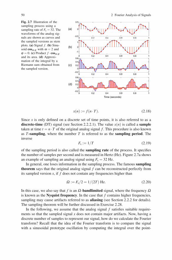
Fig. 2.7 Illustration of thesampling process using asampling rate of Fs = 32. Thewaveforms of the analog sig-nals are shown as curves andthe sampled versions as stemplots. (a) Signal f . (b) Sinu-soid cosω,ϕ with ω = 2 andϕ = 0. (c) Product f · cosω,ϕand its area. (d) Approxi-mation of the integral by aRiemann sum obtained fromthe sampled version.

(a)

(b)

(c)

Time (seconds)

(d)

x(n) := f (n ·T ). (2.18)

Since x is only defined on a discrete set of time points, it is also referred to as a

discrete-time (DT) signal (see Section 2.2.2.1). The value x(n) is called a sampletaken at time t = n ·T of the original analog signal f . This procedure is also known

as T -sampling, where the number T is referred to as the sampling period. The

inverse

Fs := 1/T (2.19)

of the sampling period is also called the sampling rate of the process. It specifies

the number of samples per second and is measured in Hertz (Hz). Figure 2.7a shows

an example of sampling an analog signal using Fs = 32 Hz.

In general, one loses information in the sampling process. The famous samplingtheorem says that the original analog signal f can be reconstructed perfectly from

its sampled version x, if f does not contain any frequencies higher than

Ω := Fs/2 = 1/(2T ) Hz. (2.20)

In this case, we also say that f is an Ω -bandlimited signal, where the frequency Ωis known as the Nyquist frequency. In the case that f contains higher frequencies,

sampling may cause artifacts referred to as aliasing (see Section 2.2.2 for details).

The sampling theorem will be further discussed in Exercise 2.28.

In the following, we assume that the analog signal f satisfies suitable require-

ments so that the sampled signal x does not contain major artifacts. Now, having a

discrete number of samples to represent our signal, how do we calculate the Fourier

transform? Recall that the idea of the Fourier transform is to compare the signal

with a sinusoidal prototype oscillation by computing the integral over the point-


wise product (see (2.12)). Therefore, in the digital domain, it seems reasonable to

sample the sinusoidal prototype oscillation in the same fashion as the signal (see

Figure 2.7b). By multiplying the two sampled functions in a pointwise fashion, we

obtain a sampled product (see Figure 2.7c). Finally, integration in the analog case

becomes summation in the discrete case, where the summands need to be weighted

by the sampling period T . As a result, one obtains the following approximation:

∑n∈Z

T f (nT )exp(−2πiωnT )≈ f̂ (ω). (2.21)

In mathematical terms, the sum can be interpreted as the overall area of rectangular

shapes that approximates the area corresponding to the integral (see Figure 2.7d).

Such an approximation is also known as a Riemann sum. As we will show in

Section 2.3.4, the quality of the approximation is good for “well-behaved” signals

f and “small” frequency parameters ω .

One defines a discrete version of the Fourier transform for a given DT-signal

x : Z→ R by setting

x̂(ω) := ∑n∈Z

x(n)exp(−2πiωn). (2.22)

In this definition, where a simple 1-sampling (i.e., T -sampling with T = 1) of the

exponential function is used, one does not assume that one knows the relation be-

tween x and the original signal f . If one is interested in recovering the relation to

the Fourier transform f̂ , one needs to know the sampling period T . Based on (2.21),

an easy calculation shows that

x̂(ω)≈ 1

Tf̂(ω

T

). (2.23)

In this approximation, the frequency parameter ω used for x̂ corresponds to the fre-

quency ω/T for f̂ . In particular, ω = 1/2 for x̂ corresponds to the Nyquist frequency

Ω = 1/(2T ) of the sampling process. Therefore, assuming that f is bandlimited by

Ω = 1/(2T ), one needs to consider only the frequencies with 0 ≤ ω ≤ 1/2 for x̂. In

the digital case, all other frequency parameters are redundant and yield meaningless

approximations.

For doing computations on digital machines, we still have some problems. One

problem is that the sum in (2.22) involves an infinite number of summands. Another

problem is that the frequency parameter ω is a continuous parameter. For both prob-

lems, there are some pragmatic solutions. Regarding the first problem, we assume

that most of the relevant information of f is limited to a certain duration in time.2

For example, a music recording of a song hardly lasts for more than ten minutes.

Having a finite duration means that the analog signal f is assumed to be zero outside

a compact interval. By possibly shifting the signal, we may assume that this interval

starts at time t = 0. This means that we only need to consider a finite number of

2 Strictly speaking, this assumption is problematic since it conflicts with the requirement of fbeing bandlimited. A mathematical fact states that there are no functions that are both limited infrequency (bandlimited) and limited in time (having finite duration).


samples x(0),x(1), . . . ,x(N − 1) for some suitable number N ∈ N. As a result, the

sum in (2.22) becomes finite.

Regarding the second problem, one computes the Fourier transform only for a

finite number of frequencies. Similar to the sampling of the time axis, one typi-

cally samples the frequency axis by considering the frequencies ω = k/M for some

suitable M ∈ N and k ∈ [0 : M−1]. In practice, one often couples the number Nof samples and the number M that determines the frequency resolution by setting

N = M. Note that the two numbers N and M refer to different aspects. However,

the coupling is convenient. It not only makes the resulting transform invertible, but

also leads to a computationally efficient algorithm, as we will see in Section 2.4.3.

Setting X(k) := x̂(k/N) and assuming that x(0),x(1), . . . ,x(N − 1) are the relevant

samples (all others being zero), we obtain from (2.22) the formula

X(k) = x̂(k/N) =N−1

∑n=0

x(n)exp(−2πikn/N) (2.24)

for integers k ∈ [0 : M−1] = [0 : N −1]. This transform is also known as the dis-crete Fourier transform (DFT), which is covered in Section 2.4.

Next, let us have a look at the frequency information supplied by the Fourier co-

efficient X(k). By (2.23) the frequency ω of x̂ corresponds to ω/T of f̂ . Therefore,

the index k of X(k) corresponds to the physical frequency

Fcoef(k) :=k

N ·T =k ·Fs

N(2.25)

given in Hertz. As we will discuss in Section 2.4.4, the coefficients X(k) need to be

taken with care. First, the approximation quality in (2.23) may be rather poor, in par-

ticular for frequencies close to the Nyquist frequency. Second, for a real-valued sig-

nal x, the Fourier transform fulfills certain symmetry properties (see Exercise 2.24).

As a result, the upper half of the Fourier coefficients are redundant, and one only

needs to consider the coefficients X(k) for k ∈ [0 : �N/2�]. Note that, in the case of

an even number N, the index k = N/2 corresponds to Fcoef(k) = Fs/2, which is the

Nyquist frequency of the sampling process.

Finally, we consider some efficiency issues when computing the DFT. To com-

pute a single Fourier coefficient X(k), one requires a number of multiplications and

additions linear in N. Therefore, to compute all coefficients X(k) for k ∈ [0 : N/2]one after another, one requires a number of operations on the order of N2. Despite

being a finite number of operations, such a computational approach is too slow for

many practical applications, in particular when N is large.

The number of operations can be reduced drastically by using an efficient algo-

rithm known as the fast Fourier transform (FFT). The FFT algorithm, which was

discovered by Gauss and Fourier two hundred years ago, has changed whole indus-

tries and is now being used in billions of telecommunication and other devices. The

FFT exploits redundancies across sinusoids of different frequencies to jointly com-

pute all Fourier coefficients by a recursion. This recursion works particularly well in

the case that N is a power of two. As a result, the FFT reduces the overall number of


operations from the order of N2 to the order of N log2 N. The savings are enormous.

For example, using N = 210 = 1024, the FFT requires roughly N log2 N = 10240 in-

stead of N2 = 1048576 operations in the naive approach—a savings factor of about

100. In the case of N = 220, the savings amount to a factor of about 50000 (see

Exercise 2.6). In Section 2.4.3, we discuss the algorithmic details of the FFT.

2.1.4 Short-Time Fourier Transform

The Fourier transform yields frequency information that is averaged over the entire

time domain. However, the information on when these frequencies occur is hidden

in the transform. We have already seen this phenomenon in Figure 2.6a, where the

change in frequency is not revealed when looking at the magnitude of the Fourier

transform. To recover the hidden time information, Dennis Gabor introduced in the

year 1946 the short-time Fourier transform (STFT). Instead of considering the

entire signal, the main idea of the STFT is to consider only a small section of the

signal. To this end, one fixes a so-called window function, which is a function that

is nonzero for only a short period of time (defining the considered section). The

original signal is then multiplied with the window function to yield a windowedsignal. To obtain frequency information at different time instances, one shifts the

window function across time and computes a Fourier transform for each of the re-

sulting windowed signals.

This idea is illustrated by Figure 2.8, which continues our example from

Figure 2.6a. To obtain local sections of the original signal, one multiplies the sig-

nal with suitably shifted rectangular window functions. In Figure 2.8b, the resulting

local section only contains frequency content at 1 Hz, which leads to a single main

peak in the Fourier transform at ω = 1. Further shifting the time window to the right,

the resulting section contains 1 Hz as well as 5 Hz components (see Figure 2.8c).

These components are reflected by the two peaks at ω = 1 and ω = 5. Finally, the

section shown in Figure 2.8d only contains frequency content at 5 Hz.

Already at this point, we want to emphasize that the STFT reflects not only the

properties of the original signal but also those of the window function. First of all,

the STFT depends on the length of the window, which determines the size of the

section. Then, the STFT is influenced by the shape of the window function. For

example, the sharp edges of the rectangular window typically introduce “ripple”

artifacts. In Section 2.5.1, we discuss such issues in more detail. In particular, we

introduce more suitable, bell-shaped window functions, which typically reduce such

artifacts.

In Section 2.5, one finds a detailed treatment of the analog and discrete versions

of the STFT and their relationship. In the following, we only consider the discrete

case and specify the most important mathematical formulas as needed in practi-

cal applications. Let x : Z→ R be a real-valued DT-signal obtained by equidistant

sampling with respect to a fixed sampling rate Fs given in Hertz. Furthermore, let

w : [0 : N −1] → R be a sampled window function of length N ∈ N. For example,



(a)

(b)

(c)

(d)

Fig. 2.8 Signal and Fourier transform consisting of two subsequent sinusoids of frequency 1 Hzand 5 Hz (see Figure 2.6a). (a) Original signal. (b) Windowed signal centered at t = 3. (c) Win-dowed signal centered at t = 5. (d) Windowed signal centered at t = 7.

in the case of a rectangular window one has w(n) = 1 for n ∈ [0 : N −1]. Implicitly,

one assumes that w(n) = 0 for all other time parameters n ∈ Z \ [0 : N −1] outside

this window. The length parameter N determines the duration of the considered sec-

tions, which amounts to N/Fs seconds. One also introduces an additional parameter

H ∈ N, which is referred to as the hop size. The hop size parameter is specified in

samples and determines the step size in which the window is to be shifted across the

signal.

With regard to these parameters, the discrete STFT X of the signal x is given by

X (m,k) :=N−1

∑n=0

x(n+mH)w(n)exp(−2πikn/N) (2.26)

with m ∈ Z and k ∈ [0 : K]. The number K = N/2 (assuming that N is even) is

the frequency index corresponding to the Nyquist frequency. The complex number

X (m,k) denotes the kth Fourier coefficient for the mth time frame. Note that for

each fixed time frame m, one obtains a spectral vector of size K + 1 given by the

coefficients X (m,k) for k ∈ [0 : K]. The computation of each such spectral vector

amounts to a DFT of size N as in (2.24), which can be done efficiently using the

FFT.


What have we actually computed in (2.26) in relation to the original analog signal

f ? As for the temporal dimension, each Fourier coefficient X (m,k) is associated

with the physical time position

Tcoef(m) :=m ·H

Fs(2.27)

given in seconds. For example, for the smallest possible hop size H = 1, one obtains

Tcoef(m) = m/Fs = m · T sec. In this case, one obtains a spectral vector for each

sample of the DT-signal x, which results in a huge increase in data volume. Further-

more, considering sections that are only shifted by one sample generally yields very

similar spectral vectors. To reduce this type of redundancy, one typically relates the

hop size to the length N of the window. For example, one often chooses H = N/2,

which constitutes a good trade-off between a reasonable temporal resolution and

the data volume comprising all generated spectral coefficients. As for the frequency

dimension, we have seen in (2.25) that the index k of X (m,k) corresponds to the

physical frequency

Fcoef(k) :=k ·Fs

N(2.28)

given in Hertz.

Before we look at some concrete examples, we first introduce the concept of a

spectrogram, which we denote by Y . The spectrogram is a two-dimensional repre-

sentation of the squared magnitude of the STFT:

Y(m,k) := |X (m,k)|2. (2.29)

It can be visualized by means of a two-dimensional image, where the horizontal

axis represents time and the vertical axis represents frequency. In this image, the

spectrogram value Y(m,k) is represented by the intensity or color in the image at

the coordinate (m,k). Note that in the discrete case, the time axis is indexed by the

frame indices m and the frequency axis is indexed by the frequency indices k.

Continuing our running example from Figure 2.8, we now consider a sampled

version of the analog signal using a sampling rate of Fs = 32 Hz. Having a physical

duration of 10 sec, this results in 320 samples (see Figure 2.9a). Using a window

length of N = 64 samples and a hop size of H = 8 samples, we obtain the spectro-

gram as shown in Figure 2.9b. In the image, the shade of gray encodes the magnitude

of a spectral coefficient, where darker colors correspond to larger values. By (2.27),

the mth frame corresponds to the physical time Tcoef(m) = m/4 sec. In other words,

the STFT has a time resolution of four frames per second. Furthermore, by (2.28),

the kth Fourier coefficient corresponds to the physical frequency Fcoef(k) := k/2 Hz.

In other words, one obtains a frequency resolution of two coefficients per Hertz.

The plots of the waveform and the spectrogram with the physically correct time and

frequency axes are shown in Figure 2.9c and Figure 2.9d, respectively.

Let us consider some typical settings as encountered when processing music

signals. For example, in the case of CD recordings one has a sampling rate of

Fs = 44100 Hz. Using a window length of N = 4096 and a hop size of H = N/2,


Time (seconds)

Time (seconds)

Index (frames)

Index (samples)

Freq

uenc

y(H

z)

Inde

x (fr

eque

ncy)

(a)

(b)

(c)

(d)

Fig. 2.9 DT-signal sampled with Fs = 32 Hz and STFT using a window length of N = 64 and ahop size of H = 8. (a) DT-signal with time axis given in samples. (b) STFT with time axis given inframes and frequency axis given in indices. (c) DT-signal with time axis given in seconds. (d) STFTwith time axis given in seconds and frequency axis given in Hertz.

this results in a time resolution of H/Fs ≈ 46.4 ms by (2.27) and a frequency res-

olution of Fs/N ≈ 10.8 Hz by (2.28). To obtain a better frequency resolution, one

may increase the window length N. This, however, leads to a poorer localization in

time so that the resulting STFT loses its capability of capturing local phenomena

in the signal. This kind of trade-off is further discussed in Section 2.5.2 and in the

exercises.

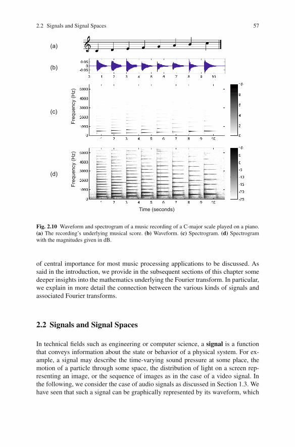
We close this section with a further example shown in Figure 2.10, which is

a recording of a C-major scale played on a piano. The first note of this scale is

C4, which we have already considered in Figure 2.1. In Figure 2.10c, the spectro-

gram representation of the recording is shown, where the time and frequency axes

are labeled in a physically meaningful way. The spectrogram reveals the frequency

information of the played notes over time. For each note, one can observe hori-

zontal lines that are stacked on top of each other. As discussed in Section 1.3.4,

these equally spaced lines correspond to the partials, the integer multiples of the

fundamental frequency of a note. Obviously, the higher partials contain less and

less of the signal’s energy. Furthermore, the decay of each note over time is re-

flected by the fading out of the horizontal lines. To enhance small sound compo-

nents that may still be perceptually relevant, one often uses a logarithmic dB scale

(see Section 1.3.3). Figure 2.10d illustrates the effect when applying the dB scale to

the values of the spectrogram. Besides an enhancement of the higher partials, one

can now observe vertical structures at the notes’ onset positions. These structures

correspond to the noise-like transients that occur in the attack phase of the piano

sound (see Section 1.3.4).

This concludes our “nutshell section” covering the most important definitions

and properties of the Fourier transform as needed for the subsequent chapters of this

book. In particular, the formula (2.26) of the discrete STFT as well as the physical

interpretation of the time parameter (2.27) and the frequency parameter (2.28) are

2.2 Signals and Signal Spaces 57

(b)

(c)

(d)

Freq

uenc

y(H

z)

Time (seconds)

Freq

uenc

y(H

z)

(a)

Fig. 2.10 Waveform and spectrogram of a music recording of a C-major scale played on a piano.(a) The recording’s underlying musical score. (b) Waveform. (c) Spectrogram. (d) Spectrogramwith the magnitudes given in dB.

of central importance for most music processing applications to be discussed. As

said in the introduction, we provide in the subsequent sections of this chapter some

deeper insights into the mathematics underlying the Fourier transform. In particular,

we explain in more detail the connection between the various kinds of signals and

associated Fourier transforms.

2.2 Signals and Signal Spaces

In technical fields such as engineering or computer science, a signal is a function

that conveys information about the state or behavior of a physical system. For ex-

ample, a signal may describe the time-varying sound pressure at some place, the

motion of a particle through some space, the distribution of light on a screen rep-

resenting an image, or the sequence of images as in the case of a video signal. In

the following, we consider the case of audio signals as discussed in Section 1.3. We

have seen that such a signal can be graphically represented by its waveform, which

Meinard MüllerFundamentals of Music ProcessingAudio, Analysis, Algorithms, Applications2015, XXIX, 487 p. 249 illus., 30 illus. in color, hardcoverISBN: 978-3-319-21944-8

http://www.springer.com/978-3-319-21944-8

Accompanying website: www.music-processing.de

This textbook provides both profound technological knowledge and a comprehensivetreatment of essential topics in music processing and music information retrieval. Includingnumerous examples, figures, and exercises, this book is suited for students, lecturers, andresearchers working in audio engineering, computer science, multimedia, and musicology

Meinard Müller is professor at the International Audio Laboratories Erlangen, Germany, a joint institution of the Friedrich-Alexander-Universität Erlangen-Nürnberg (FAU) and the Fraunhofer Institute forIntegrated Circuits IIS.

chapter 2 fourier analysis of signals - audiolabs-erlangen.de · 2016-01-15 · chapter 2 fourier...

Documents