chapter 2: continuum mechanics models and development of …
TRANSCRIPT

5 ISBN: 978-81-936820-9-8
Thesis DOI: 10.21467/books.75
AIJR Books
Chapter 2: Continuum Mechanics Models and Development of
VUMAT
Introduction
The finite element analysis of many sheet forming problems faces often difficulties due to the
strongly non-linear material behavior including friction which makes convergence difficult in
implicit finite element schemes. Such problems can be better addressed within the framework
of explicit schemes (such as ABAQUS/Explicit) especially when coupled with a remeshing
strategy. The library of ABAQUS contains several constitutive models including isotropic
hardening model kinematic hardening model and combined hardening model. Unfortunately,
the version available in ABAQUS is not versatile enough as a number of parameters are
considered to be constant. This problem is addressed in ABAQUS/Standard with the used of
field variables and user subroutine “USDFLD” which is not available in EXPLICIT.
For this reason, we developed a VUMAT user subroutine for the most general version of
combined isotropic/ kinematic hardening model for ABAQUS/EXPLICIT. In this chapter,
we firstly present a summary of the combined hardening model and its calibration, as well as
an integration model for the model and then we propose the modification of combined
hardening model to predict correctly the stress-strain curves with reverted load and its
validation.
Constitutive Models
In this study, the program is written in modular form so that different material models can be
added in the future. At the present time there are seven continuum material models, although
the isothermal elastic/plastic model is the only continuum model described here.
The main assumption is that the strain rate is constant from time tn_l to tn. During each
conjugate gradient iteration, the latest values of the kinematic quantities are used to update the
stress. All material models are written in terms of the un-rotated Cauchy stress and the
deformation rate d in the un-rotated configuration. When calculating linear elastic material
response, Hooke’s law is used. In a rate form, this is written as
�̇� = 𝜆𝑡𝑟𝑎𝑐𝑒(𝑑)𝛿 + 2𝜇𝑑 (2.1)
where and are the elastic Lame material constants.

Chapter 2: Continuum Mechanics Models and Development of VUMAT
Combined Hardening Behavior for Sheet Metal and its Application
6
2.2.1 Basic Definitions and Assumptions
Some definitions and assumptions are outlined here. In Figure 2.1, which geometrically depicts
the yield surface in deviatoric stress space, the back stress (the center of the yield surface) is
defined by the tensor If is the current value of the stress, the deviatoric part of the current
stress is
𝑆 = 𝜎 −1
3𝑡𝑟𝑎𝑐𝑒(𝜎)𝛿 (2.2)
Figure 2.1: Yield surface in deviatoric stress space.
The stress difference is then measured by subtracting the backstress from the deviatoric stress
by
𝜉 = 𝑆 − 𝛼 (2.3)
The magnitude of the deviatoric stress difference R is defined by
𝑅 = ‖𝜉‖ = √𝜉 : 𝜉 (2.4)
where the inner product of second order tensors is S : S = SijSjj. Note that if the back stress is
zero (isotropic hardening case) the stress difference is equal to the deviatoric part of the
current stress S.
The von Mises yield surface is defined as
𝑓(𝜎) =1
2𝜉 : 𝜉 = 𝜅2 (2.5)
and the von Mises effective stress is defined by
�̄� = √3
2𝜉 : 𝜉 (2.6)
Chapter 2: Continuum Mechanics Models and Development of VUMAT
Combined Hardening Behavior for Sheet Metal and its Application
7
Since R is the magnitude of the deviatoric stress tensor when = 0, it follows that
𝑅 = √2𝜅 = √2
3�̄� (2.7)
The normal to the yield surface can be determined from Equation 2.5:
𝑸 =𝝏𝒇/𝝏𝝈
‖𝝏𝒇/𝝏𝝈‖=
𝝃
𝑹 (2.8)
It is assumed that the strain rate can be decomposed into elastic and plastic parts by an additive
decomposition,
𝑑 = 𝑑𝑒𝑙 + 𝑑𝑝𝑙 (2.9)
and that the plastic part of the strain rate is given by a normality condition,
𝑑𝑝𝑙 = 𝛾𝑄 (2.10)
where the scalar multiplier is to be determined.
A scalar measure of equivalent plastic strain rate is defined by
�̄�𝑝𝑙 = √2
3𝑑𝑝𝑙 : 𝑑𝑝𝑙 (2.11)
which is chosen such that
�̄��̄�𝑝𝑙 = 𝜎 : 𝛥 휀𝑝𝑙 (2.12)
The stress is expressed in rate is assumed to be purely due to the elastic part of the strain rate
and terms of Hooke’s law by
�̇� = 𝜆𝑡𝑟𝑎𝑐𝑒(𝑑𝑒𝑙)𝛿 + 2𝜇𝑑𝑒𝑙 (2.13)
where and are the Lame constants for the material.
In what follows, the theory of isotropic hardening, kinematic hardening, and combined
hardening is described.
Chapter 2: Continuum Mechanics Models and Development of VUMAT
Combined Hardening Behavior for Sheet Metal and its Application
8
2.2.2 Isotropic Hardening
In the isotropic hardening case, the back-stress is zero and the stress difference is equal to the
deviatoric stress S. The consistency condition is written by taking the rate of Equation 2.5:
𝑓̇(𝜎) = 2𝜅�̇� (2.14) The consistency condition requires that the state of stress must remain on the yield surface at
all times. The chain rule and the definition of the normal to the yield surface given by Equation
2.8 is used to obtain
𝑓̇(𝜎) =𝜕𝑓
𝜕𝜎: �̇� = ‖
𝜕𝑓
𝜕𝜎‖𝑄 : �̇� (2.15)
and from Equations 2.4 and 2.5,
‖𝜕𝑓
𝜕𝜎‖ = ‖𝑆‖ = 𝑅 (2.16)
Combining Equations 2.14, 2.15, and 2.16,
1
𝑅𝑆 : �̇� = �̇� (2.17)
Note that because S is deviatoric, 𝑆 : �̇� = 𝑆 : �̇�, and
𝑆 : �̇� =𝑑
𝑑𝑡(1
2𝑆 : 𝑆) =
𝑑
𝑑𝑡(�̄�2
3) =
2
3�̄��̇� (2.18)
Then Equation 2.17 can be written as
�̇� = √2
3�̇̄� = √
2
3𝐻′�̄�𝑝𝑙 (2.19)
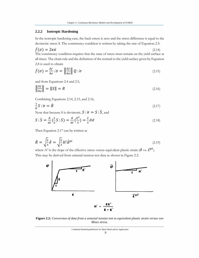
where H’ is the slope of the effective stress versus equivalent plastic strain (�̄� vs. 휀̄𝑝𝑙). This may be derived from uniaxial tension test data as shown in Figure 2.2.
Figure 2.2: Conversion of data from a uniaxial tension test to equivalent plastic strain versus von
Mises stress.

Chapter 2: Continuum Mechanics Models and Development of VUMAT
Combined Hardening Behavior for Sheet Metal and its Application
9
The consistency condition (Equation 2.17) and Equation 2.19 result in
√2
3𝐻′�̄�𝑝𝑙 = 𝑄 : �̇� (2.20)
The trial elastic stress rate �̇�𝑡𝑟 is defined by
�̇�𝑡𝑟 = 𝐶 : 𝑑 (2.21)
where C is the fourth-order tensor of elastic coefficients defined by Equation 2.13. Combining
the strain rate decomposition defined in Equation 2.9 with Equations 2.20 and 2.21 yields
√2
3𝐻′�̄�𝑝𝑙 = 𝑄 : �̇�𝑡𝑟 − 𝑄 : 𝐶 : 𝑑𝑝𝑙 (2.22)
Since Q is deviatoric, C: Q = Q and Q: C: Q = 2. Then using the normality condition
(Equation 2.10), the definition of equivalent plastic strain (Equation 2.11), and Equation 2.22,
2
3𝐻′𝛾 = 𝑄 : �̇�𝑡𝑟 − 2𝜇𝛾 (2.23)
and since Q is deviatoric (𝑄 : �̇�𝑡𝑟 = 2𝜇𝑄 : 𝑑), is determined from Equation 2.23 as
𝛾 =1
(1+𝐻′
3𝜇)𝑄 : 𝑑 (2.24)
The current normal to the yield surface Q and the total strain rate d are known quantities.
Hence, from Equation 2.24, can be determined and then used in Equation 2.10 to calculate
the plastic part of the strain rate. With the additive strain rate decomposition and the elastic
stress rate of Equations 2.9 and 2.13, this completes the definition of the rate Equations.
The means of integrating the rate Equations, subject to the constraint that the stress must
remain on the yield surface, still remains to be explained. How that is accomplished will be
shown in Section 2.3.2.
2.2.3 Kinematic Hardening
For kinematic hardening, the von Mises yield condition is written in terms of the stress
difference𝜉:
𝑓(𝜉) =1
2𝜉 : 𝜉 = 𝜅2 (2.25)
It is important to remember that both 𝜉 and the back stress are deviatoric tensors.
The consistency condition for kinematic hardening is written as
𝑓̇(𝜉) = 0 (2.26)
Chapter 2: Continuum Mechanics Models and Development of VUMAT
Combined Hardening Behavior for Sheet Metal and its Application
10
because the size of the yield surface does not grow with kinematic hardening (�̇� = 0).
Using the chain rule on Equation 2.26, and
𝜕𝑓
𝜕𝜉: �̇� = 0 (2.27)
𝜕𝑓
𝜕𝜉= ‖
𝜕𝑓
𝜕𝜉‖𝑄 = 𝑅𝑄 (2.28)
Combining Equations 2.27 and 2.28 and assuming that R # 0,
𝑄 : �̇� = 0 (2.29) or
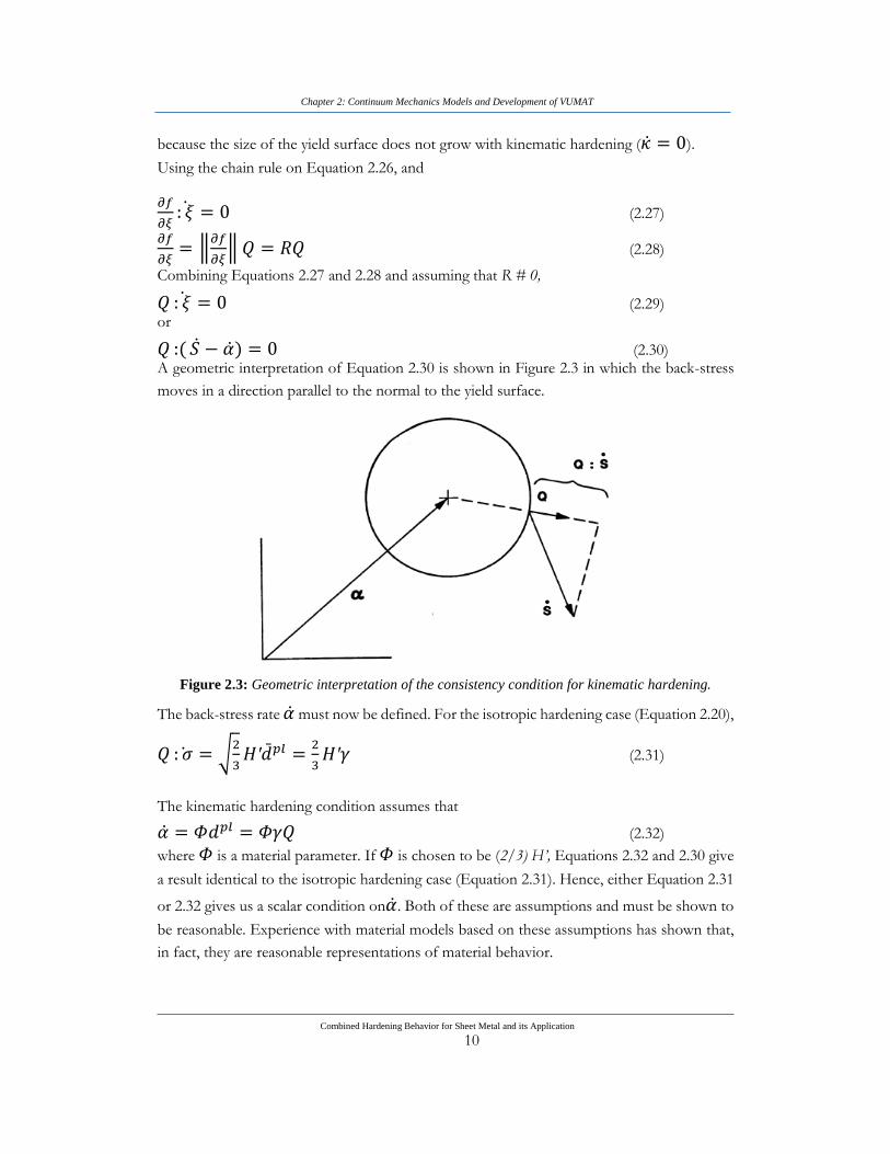
𝑄 :( �̇� − �̇�) = 0 (2.30) A geometric interpretation of Equation 2.30 is shown in Figure 2.3 in which the back-stress
moves in a direction parallel to the normal to the yield surface.
Figure 2.3: Geometric interpretation of the consistency condition for kinematic hardening.
The back-stress rate �̇� must now be defined. For the isotropic hardening case (Equation 2.20),
𝑄 : �̇� = √2
3𝐻′�̄�𝑝𝑙 =
2
3𝐻′𝛾 (2.31)
The kinematic hardening condition assumes that
�̇� = 𝛷𝑑𝑝𝑙 = 𝛷𝛾𝑄 (2.32)
where 𝛷 is a material parameter. If 𝛷 is chosen to be (2/3) H’, Equations 2.32 and 2.30 give
a result identical to the isotropic hardening case (Equation 2.31). Hence, either Equation 2.31
or 2.32 gives us a scalar condition on�̇�. Both of these are assumptions and must be shown to
be reasonable. Experience with material models based on these assumptions has shown that,
in fact, they are reasonable representations of material behavior.
Chapter 2: Continuum Mechanics Models and Development of VUMAT
Combined Hardening Behavior for Sheet Metal and its Application
11
Using Equation 2.32, Equation 2.9 (the strain rate decomposition), and Equation 2.13 (the
elastic stress rate) in Equation 2.30 (the consistency condition for kinematic hardening) gives
𝑄 :(�̇�𝑡𝑟 − 𝐶 : 𝑑𝑝𝑙 ) = 𝑄 :2
3𝐻′𝛾𝑄 (2.33)
Using the normality condition (𝑑𝑝𝑙 = 𝛾𝑄) and the fact that Q is deviatoric, C: Q = Q.
Solving Equation 2.33 for then gives
𝛾 =1
(1+𝐻′
3𝜇)𝑄 : 𝑑 (2.34)
which is the same result as that of the isotropic hardening case.
2.2.4 Combined Isotropic and Kinematic Hardening
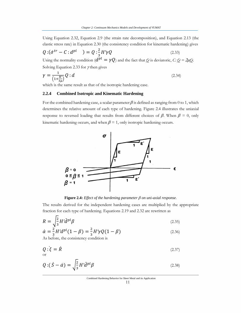
For the combined hardening case, a scalar parameter is defined as ranging from 0 to 1, which
determines the relative amount of each type of hardening. Figure 2.4 illustrates the uniaxial
response to reversed loading that results from different choices of . When = 0, only
kinematic hardening occurs, and when = 1, only isotropic hardening occurs.
Figure 2.4: Effect of the hardening parameter on uni-axial response.
The results derived for the independent hardening cases are multiplied by the appropriate
fraction for each type of hardening. Equations 2.19 and 2.32 are rewritten as
𝑅 = √2
3𝐻′�̄�𝑝𝑙𝛽 (2.35)
�̇� =2
3𝐻′𝑑𝑝𝑙(1 − 𝛽) =
2
3𝐻′𝛾𝑄(1 − 𝛽) (2.36)
As before, the consistency condition is
𝑄 : �̇� = �̇� (2.37) or
𝑄 :( �̇� − �̇�) = √2
3𝐻′�̄�𝑝𝑙𝛽 (2.38)

Chapter 2: Continuum Mechanics Models and Development of VUMAT
Combined Hardening Behavior for Sheet Metal and its Application
12
Using the elastic stress rate, the additive strain rate decomposition, and the normality
condition, 𝑄 : �̇� = 𝑄 :( �̇�𝑡𝑟 − 𝛾𝐶 : 𝑄) Together with Equations 2.36 and 2.11, this
transforms Equation 2.38 into
𝑄 : �̇�𝑡𝑟 − 𝛾𝑄 : 𝐶 : 𝑄 −2
3𝐻′𝛾𝑄(1 − 𝛽)𝑄 : 𝑄 = √
2
3𝐻′𝛽√
2
3(𝛾𝑄) :( 𝛾𝑄) (2.39)
Solving for ,
𝛾 =1
(1+𝐻′
3𝜇)𝑄 : 𝑑 (2.40)
which is the same result as was obtained for each of the independent cases.
The following is a summary of the governing Equations for the combined theory:
�̇� = 𝐶 :( 𝑑 − 𝑑𝑝𝑙) = �̇�𝑡𝑟 − 2𝜇𝛾𝑄 (2.41)
�̇� = 𝛽√2
3𝐻′�̄�𝑝𝑙 = 𝛽
2
3𝐻′𝛾 (2.42)
�̇� = (1 − 𝛽)2
3𝐻′𝑑𝑝𝑙 (2.43)
=
2
2
)(),(
)(),(0
fifplasticQ
fifelasticd pl (2.44)
𝛾 =1
(1+𝐻′
3𝜇)𝑄 : 𝑑 (2.45)
𝑄 =𝜕𝑓/𝜕𝜎
‖𝜕𝑓/𝜕𝜎‖=
𝜉
𝑅 (2.46)
Implementation of Combined Hardening Law and Development of VUMAT
The constitutive model presented in the previous section was implemented in the ABAQUS,
a general-purpose finite element program [32]. This code provides a general interface for user
programmed constitutive models through a “user subroutine” (VUMAT for
ABAQUS/Explicit). As discussed above, we develop our own user subroutine because the
versions of hardening behavior models in ABAQUS/Explicit are not flexible enough. Figure
2.5 shows schematically the integration procedure in ABAQUS/Explicit with a VUMAT. For
each time step, ABAQUS integrates the Equations of equilibriums based on the stress state at
the beginning of the step at each integration point and provides the deformation gradient for
VUMAT subroutine. VUMAT then finishes the integration of the constitutive model and
updates the stress and state variable for each integration point. With the information that
VUMAT provides, ABAQUS can then continue the calculation for the next time step.

Chapter 2: Continuum Mechanics Models and Development of VUMAT
Combined Hardening Behavior for Sheet Metal and its Application
13
Figure 2.5: ABAQUS and VUMAT subroutine.
2.3.1 Derivation of the Constitutive Equations Elasticity
A basic assumption of elastic-plastic models is that the deformation can be divided into an
elastic part and an inelastic (plastic) part. There are mainly two methods of decomposition of
kinematics: (a) multiplicative decomposition F = Fel Fpl, in which it requires that the plastic
deformation gradient Fpl (9 elements) is stored as a state variable for all integration points. (b)
additive decomposition: 𝛥휀 = 𝛥휀𝑒𝑙 + 𝛥휀𝑝𝑙where 𝛥휀is the total strain increment, 𝛥휀𝑒𝑙 is
the increment of the elastic strain, and 𝛥휀𝑝𝑙 is the increment of inelastic strain. The additive
decomposition is adequate when the elastic strains are small. For a linear and isotropic
material:
𝛥𝜎 = 𝐶𝛥휀𝑒𝑙 = 𝐶(𝛥휀 − 𝛥휀𝑝𝑙) with 𝐶 ≡ 2𝐺𝐼 + (𝐾 − 2𝐺/3)𝛿 : 𝛿 (2.47) where C is the forth order elasticity tensor, I and δ are respectively the forth and second order
identity tensor, G and K are the shear modulus and bulk modulus respectively which are

Chapter 2: Continuum Mechanics Models and Development of VUMAT
Combined Hardening Behavior for Sheet Metal and its Application
14
functions of powder porosity. For isotropic materials, 𝐺 =𝐸
2(1+𝜈) and𝐾 =
𝐸
3(1−2𝜈) where
E and ν are Young’s modulus and Poisson’s ratio, respectively.
Plasticity: The evolution Equation for the plastic part of the deformation gradient (“flow
rule”) is given by 𝛥휀̄𝑝𝑙 = 𝛥𝛾𝑄 where, 𝛥𝛾 will be determined in Section 2.3.2. The details
of time integration procedure are discussed below.
2.3.2 Integration procedure
For a typical time step, our VUMAT uses explicit Euler algorithm (Euler forward) to integrate
stresses and internal state variable. The time increment is limited by the overall stability limit
of the explicit integration of the Equations of motion. This is usually more restrictive than the
stability limit of the stress integration in the VUMAT. Other integration algorithms are also
can be used, such as implicit Euler algorithm (Euler backward) [33, 34] or semi-implicit Euler
algorithm [35]. Since the stability constrain limits the overall time increment, explicit and semi-
explicit methods (i.e. not iterative methods) are more efficient than fully implicit which are
more appropriate for large time steps and plastic strain increments. The VUMAT uses the
stress and internal variables at the beginning of an increment and the strain increment provided
by ABAQUS and needs to predict the stress at the end of the increment, as well as the new
values of the internal state variables.
The increment of strain across a time step Δt = tn+1 −tn is
𝛥휀𝑛+1 = 𝛥휀𝑛+1𝑒𝑙 + 𝛥휀𝑛+1
𝑝𝑙 (2.48)
The finite element algorithm requires an incremental form of Equations 2.41 through 2.46.
Additionally, an algorithm must be used that integrates the incremental Equations subject to
the constraint that the stress remains on the yield surface.
The incremental analogs of Equations 2.41 through 2.43 are
𝜎𝑛+1 = 𝜎𝑛+1𝑡𝑟 − 2𝜇𝛥𝛾𝑄 (2.49)
𝑅𝑛+1 = 𝑅 +𝑛2
3𝛽𝐻′𝛥𝛾 (2.50)
𝛼𝑛+1 = 𝛼𝑛 + (1 − 𝛽)2
3𝛥𝛾𝐻′𝑄 (2.51)
where 𝛥𝛾 represents the product of the time increment and the equivalent plastic strain rate
(𝛥𝛾 = 𝛾𝛥𝑡) The subscripts n and n + 1 refer to the beginning and end of a time step,
respectively; H, the slope of the uniaxial yield stress versus the plastic strain curve, is calculated
by Equations (2.52), and the scalar parameter, is defined as ranging from 0 to 1. When =
Chapter 2: Continuum Mechanics Models and Development of VUMAT
Combined Hardening Behavior for Sheet Metal and its Application
15
0, only kinematic hardening occurs, and when =1, only isotropic hardening occurs. For
isotropic/kinematic hardening, is determined by comparing cyclic tensile curves between
experiment data and simulation data.
𝐻 =𝑑�̄�
𝑑�̄�= 𝐾𝑛(휀0 + 휀�̄�𝑙)
𝑛−1 (2.52)
For nonlinear isotropic/kinematic hardening model, the size of yield surface was modified as
a function of equivalent plastic strain 휀�̄� and has the relationship with Swift’s work-hardening
law Equation (2.53) following Equation (2.54)
�̄�(휀�̄�𝑙) = 𝐾(휀0 + 휀�̄�𝑙)𝑛 ⥂ (2.53)
�̄�𝑌(휀�̄�𝑙) = �̄�(휀�̄�𝑙) − 𝐻휀�̄�𝑙 (2.54)
An incremental analog is needed for the rate forms of the consistency condition given by
Equations 2.14, 2.26, and 2.38. At the end of the time step, the stress state must be on the
yield surface. Hence, the incremental consistency condition is
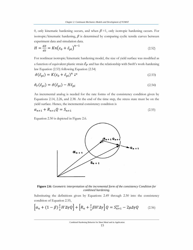
𝛼𝑛+1 + 𝑅𝑛+1𝑄 = 𝑆𝑛+1 (2.55)
Equation 2.50 is depicted in Figure 2.6.
Figure 2.6: Geometric interpretation of the incremental form of the consistency Condition for
combined hardening.
Substituting the definitions given by Equations 2.49 through 2.50 into the consistency
condition of Equation 2.55,
[𝛼𝑛 + (1 − 𝛽)2
3𝐻′𝛥𝛾𝑄] + [𝑅𝑛 +
2
3𝛽𝐻′𝛥𝛾] 𝑄 = 𝑆𝑛+1
𝑡𝑟 − 2𝜇𝛥𝛾𝑄 (2.56)

Chapter 2: Continuum Mechanics Models and Development of VUMAT
Combined Hardening Behavior for Sheet Metal and its Application
16
Taking the tensor product of both sides of Equation 2.56 with Q and solving for𝛥𝛾 ,
𝛥𝛾 =1
2𝜇
1
(1+𝐻′
3𝜇)(‖𝜉𝑛+1
𝑡𝑟 ‖ − 𝑅𝑛) (2.57)
It follows from Equation 2.57 that the plastic strain increment is proportional to the
magnitude of the excursion of the elastic trial stress past the yield surface (see Figure 2.6).
Using the result of Equation 2.57 in Equations 2.49 through 2.51 completes the algorithm. In
addition,
𝛥𝑑𝑝𝑙 = 𝛥𝛾𝑄 (2.58)
and
𝛥�̄�𝑝𝑙 = √2
3𝛥𝛾 (2.59)
Using Equation 2.57 in Equation 2.49 shows that the final stress is calculated by returning the
elastic trial stress radially to the yield surface at the end of the time step (hence the name Radial
Return Method). Estimates of the accuracy of this method and other methods for similarly
integrating the rate Equations are available in Krieg and Krieg [28] and Schreyer et al. [29].
The radial return correction (the last term in Equation 2.49) is purely deviatoric. The summary
of numerical integration algorithm of model is depicted in Figure 2.7.
Figure 2.7: Geometric interpretation of the radial returned correction.
2.3.3 Verification of VUMAT subroutine
Above constitutive model is implemented into a commercial finite element program
ABAQUS/Explicit via VUMAT user material for the uni-axial tension-compression and
compression-tension tests with standard ASTM specimens for material of magnesium alloy

Chapter 2: Continuum Mechanics Models and Development of VUMAT
Combined Hardening Behavior for Sheet Metal and its Application
17
sheet which having rectangular cross-section of 13 mm width by 3.2 thickness and a gage
length of 50 mm. in order to prevent buckling occurrence, a test method developed by Boger
et al. [9], which relies on through-thickness sheet stabilization to avoid buckling, was used to
extend the attainable strain range of Mg sheet in compression to approximately −0.08. A
schematic of the novel tension/compression test [9] and the sample dimensions are shown in
Figure 2.8 (a) two flat steel plates and a hydraulic cylinder system were used to provide side
force to support the exaggerated dog-bone specimen. Side forces of 12 kN were used to
stabilize the sheet sample. Figure 2.8 (b) shows the finite-element model of ABAQUS version
6.5 for test process. Here, the blank modeled using solid elements C3D8R, and the flat steel
plate modeled using rigid surface-elements R3D4.
Figure 2.8: Schematic of the novel tension/compression test [9]
The average element size of the solid elements was about 1mm in width, 2mm in length, and
1mm in height. Meanwhile, the average element size of the rigid surface-elements was about
2 mm in width, and 2 mm in length. The friction coefficient at the blank/flat plate interface,
2=0.1, was assumed for all the simulations. The other material parameters are listed in Table
2.1.
Table 2.1: Mechanical properties of tested material (Magnesium alloy sheet)
Material AZ31B
Density (r, kg/cm3) 1.77e-06
Young’s modulus (E, kN/cm2) 45000
Possion’s ratio 0.35
Tension yield stress (MPa) (𝜎𝑌𝑇) 220
Compression yield stress (MPa) (𝜎𝑌𝐶) 120
0.005
K (MPa) 365.09
n 0.124

Chapter 2: Continuum Mechanics Models and Development of VUMAT
Combined Hardening Behavior for Sheet Metal and its Application
18
Figure 2.9 shows the comparisons between the FE simulation and experiment results. The
best fit for uni-axial tensile test and Bauschinger effect was chosen with the scalar parameter
of 0.5. However, there are discrepancies between theoretical models and the test data in
others zone. Therefore, in this chapter we have modified the hardening law to predict correctly
behavior of stress-strain curves at reversed load for Mg alloy and also all others kind of
materials.
Figure 2.9: The comparisons between the experiment result and FE simulation results of
combined kinematic/isotropic hardening.
2.3.4 A Modification of Combined Non-linear Hardening
As shown in Figure 2.9, when changes from 0.0 to 1.0 the directions of cyclic tensile curves
will be changed. It means that, if we can present as a function of equivalent strain then we
can predict correctly the shapes of stress-strain curves at compression and reversed stress. In
this study, we proposed as exponential function of equivalent strain. In compression stress,
the scalar parameter is expressed as below:
𝛽𝐶 = 𝛽0 − 𝐹(휀𝑝𝑙(𝐶)
)𝑚 (2.60)
where 0 is the initial direction of stress-strain curves when compression stress occurs. Here,
0 = 1 is chosen to follow isotropic hardening direction. F and m are determined by fitting the
generated curve from simulation with experiment data and chosen the best fit as F of 2.016e07
and m of 5 for Mg alloy sheet.

Chapter 2: Continuum Mechanics Models and Development of VUMAT
Combined Hardening Behavior for Sheet Metal and its Application
19
In case of reversed stress occurrence for compression-tension tests, as depict in Figure 2.9,
the curve should be divided by three sections. The first section is formulated as Equation
(2.61)
𝛽𝑅1𝐶−𝑇 = 𝛽0 − 𝐹1(휀𝑅
𝑝𝑙(𝐶−𝑇))𝑚1 (2.61)
here, 0 = 1, F1 and m1 was estimated as 1.952e08 and 5 for Mg alloy sheet, respectively. The
second section is expressed as Equation (2.62) when휀𝑅𝑝𝑙(𝐶−𝑇)
is greater than 0.04 mm.
𝛽𝑅2𝐶−𝑇 = 𝐹2(휀𝑅
𝑝𝑙(𝐶−𝑇))𝑚2 (2.62)
Similarly, F2 and m2 was estimated as 1.53e03 and 0.2 for Mg alloy sheet, respectively. The
third section is generated when 𝛽𝑅2𝐶−𝑇reaches = 0.5 of fitting curve for uni-axial tensile test
then 𝛽𝑅2𝐶−𝑇 = 0.5.
Figure 2.10 (a) shows the comparison of the measured continuous uni-axial tension-
compression (T-C) and compression-tension (C–T) tests to the results calculated from the
finite element simulations with proposed models. The results of proposed model are good
agreement with measurements. Figure 2.10 (b) present the results of tension-compression (T-
C) and compression-tension (C–T) FE simulation with various of pre-strain. To investigate
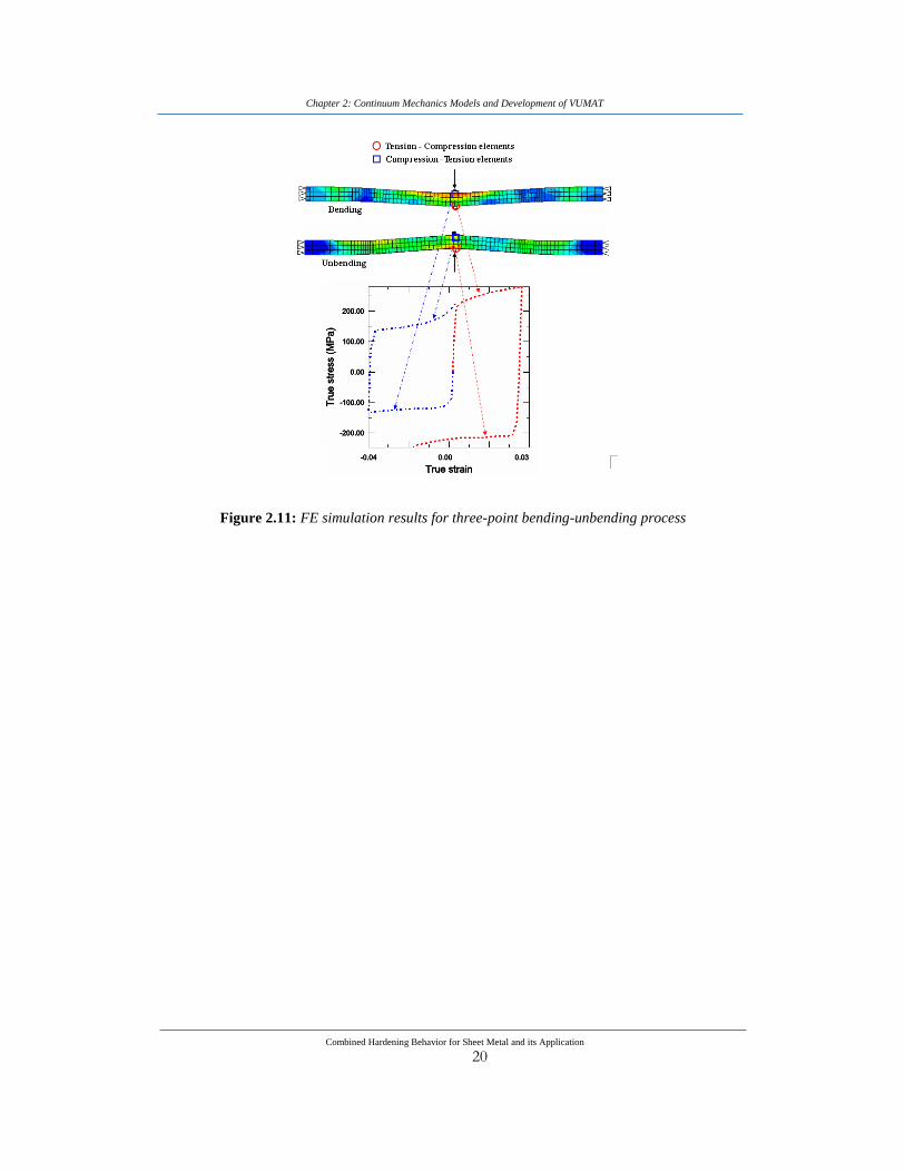
this hardening model, finite element analysis of three-point bending-unbending test for the
magnesium alloy sheet modeled using solid elements C3D8R is validated. The simulation
results are depicted and plotted in Figure 2.11. In FE simulation result of three-point bending-
unbending for solid elements, we can check tension-compression and compression-tension
curves for correlative elements at the same time. The proposed hardening law simulates
forward bending-unbending quite well comparing with tension-compression and
compression-tension test in Figure 2.10
(a) (b) Figure 2.10: Uni-axial tension-compression (T-C) and compression-tension (C–T) simulation
results of proposed model comparing with experiment data (a) and with various of pre-strain (b)
Chapter 2: Continuum Mechanics Models and Development of VUMAT
Combined Hardening Behavior for Sheet Metal and its Application
20
Figure 2.11: FE simulation results for three-point bending-unbending process