chapter 2 algorithm analysis - william & marytadavis/cs303/f16/ch02.pdf · general rules 32...
TRANSCRIPT

Chapter 2
Algorithm Analysis

Introduction
2
−algorithm
−set of simple instructions to solve a problem
−analyzed in terms, such as time and memory, required
−too long (minutes, hours, years) – no good
−too much memory (terabytes) – no good
−we can estimate resource usage using a formal
mathematical framework to count basic operations
−big-O 𝑂(𝑓(𝑁))
−big-omega Ω (𝑓(𝑁))
−big-theta Θ (𝑓 𝑁 )

Asymptotic Notation
3
− formal definitions
𝑓 𝑛 = 𝑂(𝑔(𝑛)) 𝑓 𝑛 = Ω (𝑔(𝑛)) 𝑓 𝑛 = Θ(𝑔 𝑛 )
𝑓 𝑛 and 𝑔(𝑛) are positive for 𝑛 > 1
when we say that 𝑋 is true when 𝑛 is sufficiently large, we
mean there exists 𝑁 such that 𝑋 is true for all 𝑛 > 𝑁
we are comparing relative rates of growth

Asymptotic Notation: Big-𝑂
4
𝑓 𝑛 = 𝑂(𝑔(𝑛)) if there exist constants 𝑐 and 𝑁 such that
𝑓 𝑛 ≤ 𝑐 · 𝑔(𝑛) for all 𝑛 > 𝑁
loosely speaking, 𝑓 𝑛 = 𝑂 𝑔 𝑛 is an analog of 𝑓 ≤ 𝑔
example: if 𝑓 𝑛 = 54𝑛2 + 42𝑛 and 𝑔 𝑛 = 𝑛2 then 𝑓 = 𝑂(𝑔) since
𝑓 𝑛 ≤ 55𝑔(𝑛)
for all 𝑛 > 42

Asymptotic Notation: Ω
5
𝑓 𝑛 = Ω(𝑔(𝑛)) if there exist constants 𝑐 and 𝑁 such that
𝑓 𝑛 ≥ 𝑐 · 𝑔(𝑛) for all 𝑛 > 𝑁
loosely speaking, 𝑓 𝑛 = Ω 𝑔 𝑛 is an analog of 𝑓 ≥ 𝑔

Asymptotic Notation: Θ
6
𝑓 𝑛 = Θ(𝑔(𝑛)) if there exist constants 𝑐1, 𝑐2, and 𝑁 such
that
𝑐1 · 𝑔 𝑛 < 𝑓 𝑛 < 𝑐2 · 𝑔(𝑛) for all 𝑛 > 𝑁
loosely speaking, 𝑓 𝑛 = Θ 𝑔 𝑛 is an analog of 𝑓 ≈ 𝑔
Relationship of 𝑂, Ω, and Θ
7
−note that
𝑓 𝑛 = 𝑂 𝑔 𝑛 ⇔ 𝑔 𝑛 = Ω(𝑓 𝑛 )
since
𝑓 𝑛 < 𝑐𝑔 𝑛 ⇔ 𝑔 𝑛 >1
𝑐𝑓 𝑛
−also
𝑓 𝑛 = Θ 𝑔 𝑛 ⇔ 𝑓 𝑛 = 𝑂 𝑔 𝑛 and 𝑓 𝑛 = Ω 𝑔 𝑛
since 𝑓 𝑛 = Θ(𝑔(𝑛)) means that there exist 𝑐1, 𝑐2, and 𝑁
such that
𝑐1 · 𝑔 𝑛 < 𝑓 𝑛 < 𝑐2 · 𝑔(𝑛) for all 𝑛 > 𝑁
Asymptotic Notation: First Observation
8
− for sufficiently large 𝑛,
𝑓 𝑛 = 𝑂(𝑔(𝑛)) gives an upper bound on 𝑓 in terms of 𝑔
𝑓 𝑛 = Ω (𝑔(𝑛)) gives a lower bound on 𝑓 in terms of 𝑔
𝑓 𝑛 = Θ(𝑔 𝑛 ) gives both an upper and lower bound on 𝑓
in terms of 𝑔
Asymptotic Notation: Second Observation
9
− it is the existence of constants that matters for the purposes of asymptotic complexity analysis – not the exact values of the constants
−example: all of the following imply 𝑛2 + 𝑛 = 𝑂(𝑛2):
𝑛2 + 𝑛 < 4𝑛2 for all 𝑛 > 1
𝑛2 + 𝑛 < 2𝑛2 for all 𝑛 > 1
𝑛2 + 𝑛 < 1.01𝑛2 for all 𝑛 > 100
𝑛2 + 𝑛 < 1.000001𝑛2 for all 𝑛 > 1000
Asymptotic Notation: Third Observation
10
−we typically ignore constant factors and lower-order terms, since all we want to capture is growth trends
−example:
𝑓 𝑛 = 1,000𝑛2 + 10,000𝑛 + 42
⇒ 𝑓 𝑛 = 𝑂(𝑛2)
but the following are discouraged:
𝑓 𝑛 = 𝑂(1,000𝑛2) true, but bad form
𝑓 𝑛 = 𝑂(𝑛2 + 𝑛) true, but bad form
𝑓 𝑛 < 𝑂(𝑛2) < built into 𝑂
Asymptotic Notation: Fourth Observation
11
𝑂(𝑔(𝑛)) assures that you can’t do any worse than 𝑔(𝑛), but
it can unduly pessimistic
Ω (𝑔(𝑛)) assures that you can’t do any better than 𝑔(𝑛), but
it can unduly optimistic
Θ(𝑔 𝑛 ) is the strongest statement: you can’t do any better
than 𝑔(𝑛), but you can’t do any worse

A Shortcoming of 𝑂
12
an 𝑓 𝑛 = 𝑂(𝑔(𝑛)) bound can be misleading
example: 𝑛 = 𝑂(𝑛2), since 𝑛 < 𝑛2 for all 𝑛 > 1
however, for large 𝑛, 𝑛 ≪ 𝑛2 ‒ the functions 𝑓 𝑛 = 𝑛 and
𝑔 𝑛 = 𝑛2 are nothing alike for large 𝑛
we don’t write something like 𝑓 𝑛 = 𝑂(𝑛2) if we know, say,
that 𝑓 𝑛 = 𝑂(𝑛)
upper bounds should be as small as possible!

A Shortcoming of Ω
13
an 𝑓 𝑛 = Ω(𝑔(𝑛)) bound can be misleading
example: 𝑛2 = Ω(𝑛), since 𝑛2 > 𝑛 for all 𝑛 > 1
however, for large 𝑛, 𝑛2 ≫ 𝑛 ‒ the functions 𝑓 𝑛 = 𝑛 and
𝑔 𝑛 = 𝑛2 are nothing alike for large 𝑛
we don’t write something like 𝑓 𝑛 = Ω(𝑛) if we know, say,
that 𝑓 𝑛 = Ω(𝑛2)
lower bounds should be as large as possible!
Θ is the Most Informative
14
a 𝑓 𝑛 = Θ(𝑔(𝑛)) relationship is the most informative:
𝑐1 · 𝑔 𝑛 < 𝑓 𝑛 < 𝑐2 · 𝑔(𝑛) for all 𝑛 > 𝑁
example: 2𝑛2 + 𝑛 = Θ(𝑛2)
2𝑛2 < 2𝑛2 + 𝑛 < 3𝑛2
for all 𝑛 > 1
for large values of 𝑛, the ratio (2𝑛2 + 𝑛)/𝑛2 tends to 2;
in this sense,
2𝑛2 + 𝑛 ≈ 2𝑛2

Typical Growth Rates
15
https://expcode.wordpress.com/2015/07/19/big-o-big-omega-and-big-theta-notation/
Additional Rules
16
Rule 1
if 𝑇1 𝑛 = 𝑂(𝑓(𝑛)) and 𝑇2 𝑛 = 𝑂(𝑔(𝑛)) then
(a) 𝑇1 𝑛 + 𝑇2 𝑛 = 𝑂(𝑓 𝑛 + 𝑔(𝑛)) (or just
𝑂(max (𝑓 𝑛 , 𝑔(𝑛)))
(b) 𝑇1 𝑛 ∗ 𝑇2 𝑛 = 𝑂(𝑓 𝑛 ∗ 𝑔(𝑛))
Rule 2
if 𝑇(𝑛) is a polynomial of degree 𝑘, then 𝑇 𝑛 = Θ(𝑛𝑘)
Rule 3
logk𝑛 = 𝑂 𝑛 for any constant 𝑘 (logarithms grow very slowly)

Typical Growth Rates
17
Function Name
𝑐 constant
log 𝑛 logarithmic
𝑛 linear
𝑛 log 𝑛
𝑛2 quadratic
𝑛3 cubic
2𝑛 exponential

Typical Growth Rates
18
http://www.cosc.canterbury.ac.nz/cs4hs/2015/files/complexity-tractability-julie-mcmahon.pdf

Complexity and Tractability
19
assume computer speed of 1 billion ops/sec
T(n)
n n n log n n2
n3
n4
n10
2n
10 .01ms .03ms .1ms 1ms 10ms 10s 1ms
20 .02ms .09ms .4ms 8ms 160ms 2.84h 1ms
30 .03ms .15ms .9ms 27ms 810ms 6.83d 1s
40 .04ms .21ms 1.6ms 64ms 2.56ms 121d 18m
50 .05ms .28ms 2.5ms 125ms 6.25ms 3.1y 13d
100 .1ms .66ms 10ms 1ms 100ms 3171y 4´1013
y
103
1ms 9.96ms 1ms 1s 16.67m 3.17´1013
y 32´10283
y
104
10ms 130ms 100ms 16.67m 115.7d 3.17´1023
y
105
100ms 1.66ms 10s 11.57d 3171y 3.17´1033
y
106
1ms 19.92ms 16.67m 31.71y 3.17´107y 3.17´10
43y

What to Analyze
20
in order to analyze algorithms, we need a model of
computation
−standard computer with sequential instructions
−each operation (+, -, *, /, =, etc.) takes one time unit, even
memory accesses
− infinite memory
−obviously unrealistic
Complex Arithmetic Operations
21
−examples: 𝑥𝑛 log2 𝑥 𝑥
−count the number of basic operations required to execute
the complex arithmetic operations
− for instance, we could compute 𝑥𝑛 as
𝑥𝑛 ← 𝑥 ∗ 𝑥 ∗ ⋯∗ 𝑥 ∗ 𝑥
there are 𝑛 − 1 multiplications, so there are 𝑛 − 1 basic
operations to compute 𝑥𝑛 plus one more basic operation
to assign or return the result

What to Analyze
22
different types of performance are analyzed
−best case
−may not represent typical behavior
−average case
−often reflects typical behavior
−difficult to determine what is average
−difficult to compute
−worst case
−guarantee on performance for any input
−typically considered most important
−should be implementation-independent
Maximum Subsequence Sum Problem
23
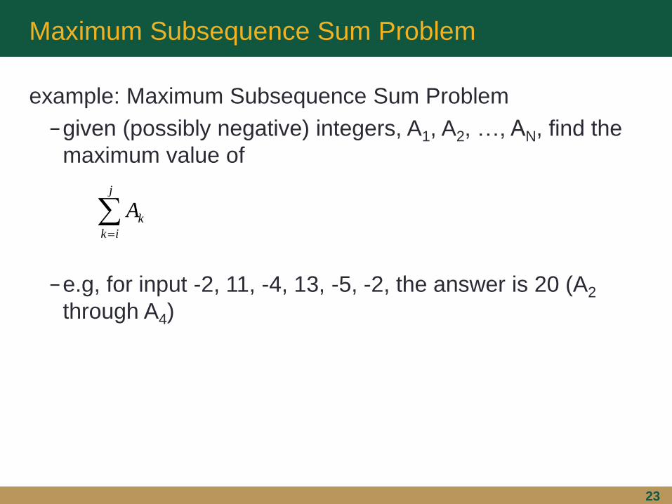
example: Maximum Subsequence Sum Problem
−given (possibly negative) integers, A1, A2, …, AN, find the
maximum value of
−e.g, for input -2, 11, -4, 13, -5, -2, the answer is 20 (A2
through A4)
j
ik
kA

Maximum Subsequence Sum Problem
24
many algorithms to solve this problem
−we will focus on four with run time in the table below

Maximum Subsequence Sum Problem
25
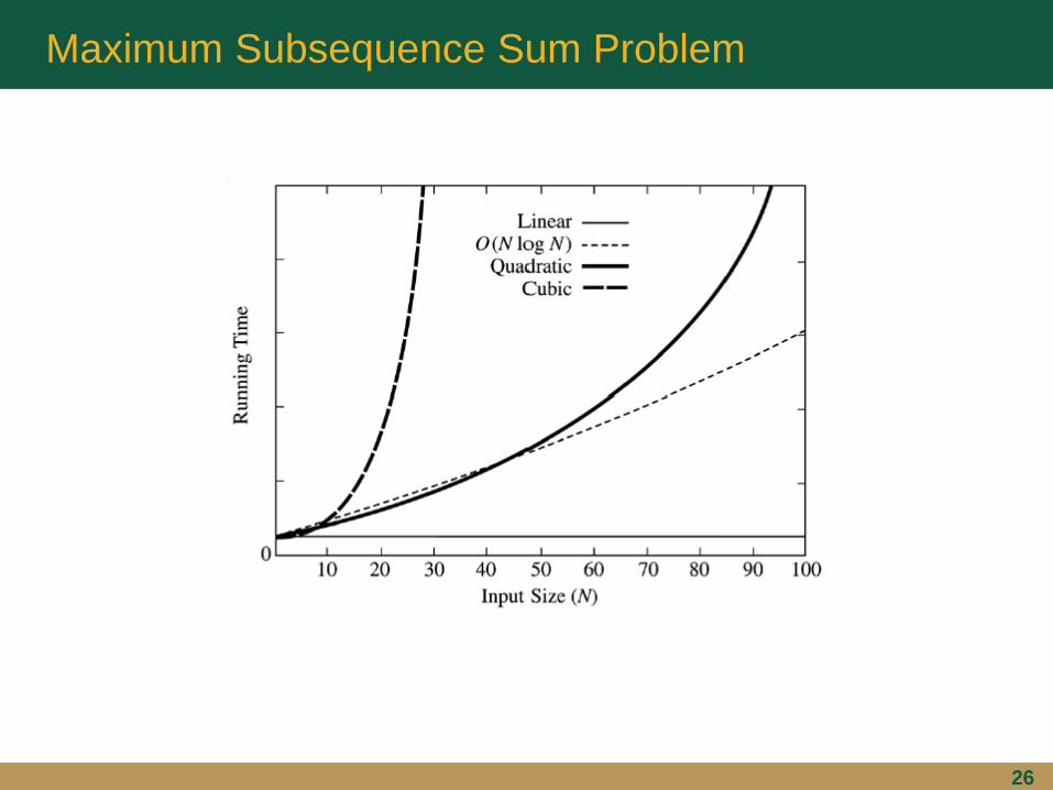
notes
−computer actually run on not important since we’re looking
to compare algorithms
− for small inputs, all algorithms perform well
− times do not include read time
−algorithm 4: time to read would surpass time to compute
−reading data is often the bottleneck
− for algorithm 4, the run time increases by a factor of 10 as
the problem size increases by a factor of 10 (linear)
−algorithm 2 is quadratic; therefore an increase of input by
a factor of 10 yields a run time factor of 100
−algorithm 1 (cubic): run time factor of 1000
Maximum Subsequence Sum Problem
26

Maximum Subsequence Sum Problem
27

Running Time Calculations
28
at least two ways to estimate the running time of a program
−empirically
−as in previous results
−realistic measurement
−analysis
−helps to eliminate bad algorithms early when several
algorithms are being considered
−analysis itself provides insight into designing efficient
algorithms
−pinpoints bottlenecks, which need special coding

A Simple Example
29
calculate 𝑖3𝑁𝑖=1
A Simple Example
30
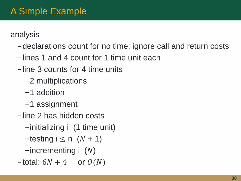
analysis
−declarations count for no time; ignore call and return costs
− lines 1 and 4 count for 1 time unit each
− line 3 counts for 4 time units
−2 multiplications
−1 addition
−1 assignment
− line 2 has hidden costs
− initializing i (1 time unit)
−testing i ≤ n (𝑁 + 1)
− incrementing i (𝑁)
− total: 6𝑁 + 4 or 𝑂(𝑁)

A Simple Example
31
analysis
− too much work to analyze all programs like this
−since we’re dealing with 𝑂, we can use shortcuts to help
− line 3 counts for 4 time units, but is 𝑂(1)
− line 1 is insignificant compared to the for loop

General Rules
32
concentrate on loops and recursive calls
−Rule 1 – FOR loops
−running time of the statements inside (including tests)
times the number of iterations
−Rule 2 – Nested loops
−analyze from the inside out
−running time of the statements times the product of the
sizes of all the loops
−watch out for loops that
−contribute only a constant amount of computation
−contain break statements
Single Loops
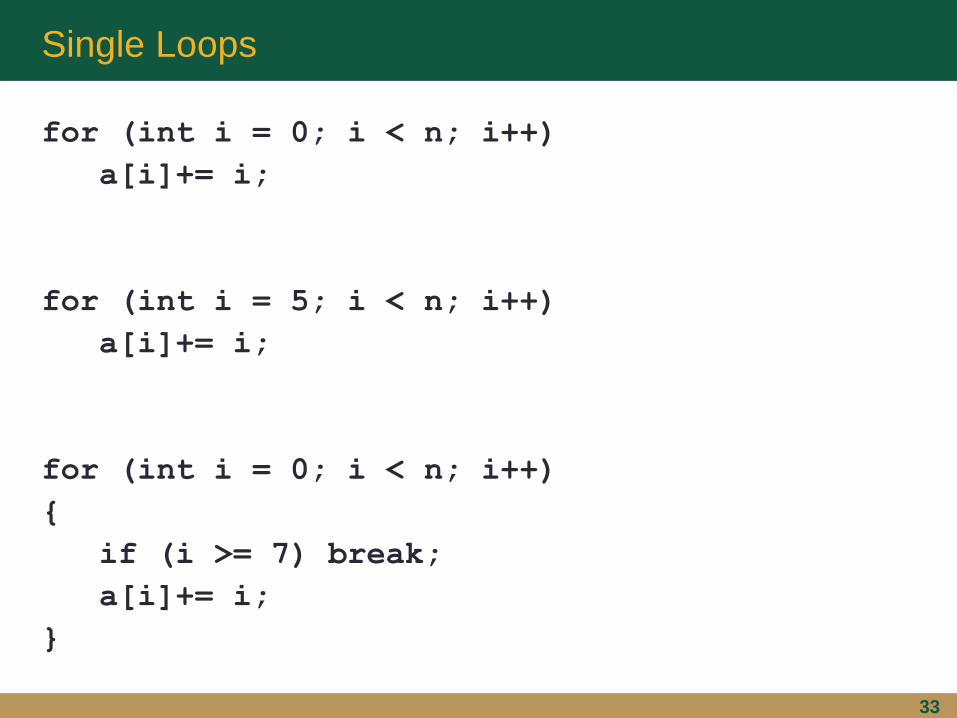
33
for (int i = 0; i < n; i++)
a[i]+= i;
for (int i = 5; i < n; i++)
a[i]+= i;
for (int i = 0; i < n; i++)
{
if (i >= 7) break;
a[i]+= i;
}

Nested Loops
34
for (int i = 0; i < n; ++i)
for (int j = 0; j < n; ++j)
++k;
−constant amount of computation inside nested loop
−must multiply number of times both loops execute
−𝑂(𝑛2)
for (int i = 0; i < n; ++i)
for (int j = i; j < n; ++j)
++k;
−even though second loop is not executed as often, still
𝑂(𝑛2)
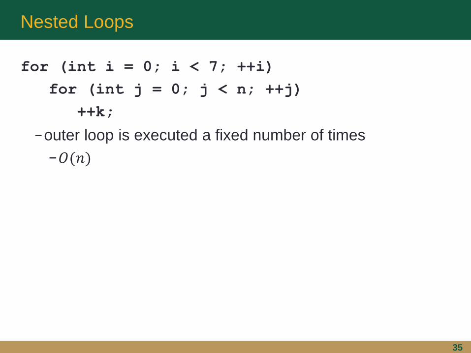
Nested Loops
35
for (int i = 0; i < 7; ++i)
for (int j = 0; j < n; ++j)
++k;
−outer loop is executed a fixed number of times
−𝑂(𝑛)
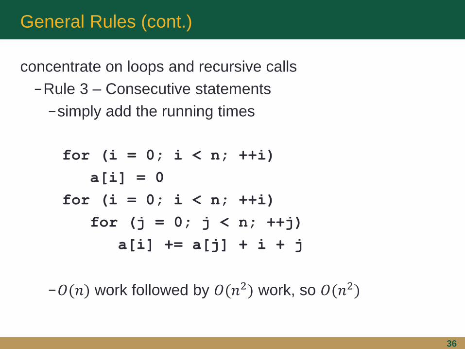
General Rules (cont.)
36
concentrate on loops and recursive calls
−Rule 3 – Consecutive statements
−simply add the running times
for (i = 0; i < n; ++i)
a[i] = 0
for (i = 0; i < n; ++i)
for (j = 0; j < n; ++j)
a[i] += a[j] + i + j
−𝑂(𝑛) work followed by 𝑂(𝑛2) work, so 𝑂(𝑛2)

General Rules (cont.)
37
concentrate on loops and recursive calls
−Rule 4 – if/else
if (test)
S1
else
S2
−total running time includes the test plus the larger of the
running times of S1 and S2
−could be overestimate in some cases, but never an
underestimate

General Rules (cont.)
38
concentrate on loops and recursive calls
− function calls analyzed first
− recursion
− if really just a for loop, not difficult (the following is 𝑂(𝑛))
long factorial (int n)
{
if (n <= 1)
return 1;
else
return n * factorial (n – 1);
}

General Rules (cont.)
39
previous example not a good use of recursion
− if recursion used properly, difficult to convert to a simple
loop structure
what about this example?
long fib (int n)
{
if (n <= 1)
return 1;
else
return fib(n – 1) + fib (n – 2);
}

General Rules (cont.)
40
even worse!
−extremely inefficient, especially for values > 40
−analysis
−for 𝑁 = 0 or 𝑁 = 1, 𝑇(𝑁) is constant: 𝑇(0) = 𝑇(1) = 1
−since the line with recursive calls is not a simple
operation, it must be handled differently
𝑇 𝑁 = 𝑇 𝑁 − 1 + 𝑇 𝑁 − 2 + 2 for 𝑁 ≥ 2
−we have seen that this algorithm <5
3
𝑁
−similarly, we could show it is >3
2
𝑁
−exponential!
General Rules (cont.)
41
with current recursion
− lots of redundant work
−violating compound interest rule
− intermediate results thrown away
running time can be reduced substantially with simple for loop

Maximum Subsequence Sum Problem Revisited
42
example: Maximum Subsequence Sum Problem
−given (possibly negative) integers, A1, A2, …, AN, find the
maximum value of
−e.g, for input -2, 11, -4, 13, -5, -2, the answer is 20 (A2
through A4)
−previously, we reviewed running time results for four
algorithms
j
ik
kA
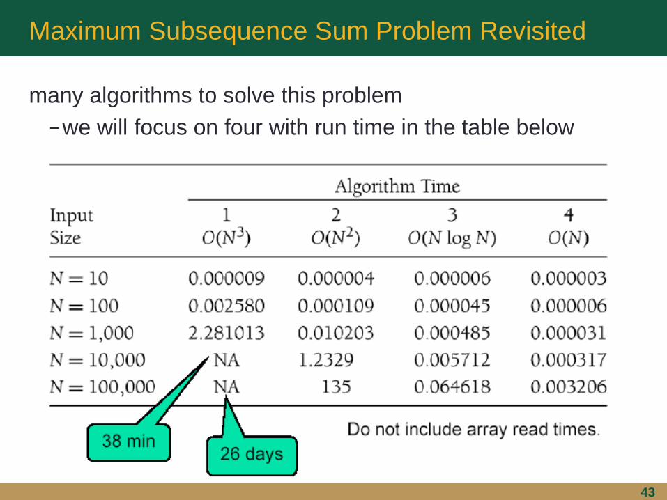
Maximum Subsequence Sum Problem Revisited
43
many algorithms to solve this problem
−we will focus on four with run time in the table below

Maximum Subsequence Sum Problem Revisited
44

Algorithm 1
45

Algorithm 1
46
exhaustively tries all possibilities
− first loop iterates 𝑁 times
−second loop iterates 𝑁 − 𝑖 times, which could be small,
but we must assume the worst
− third loop iterates 𝑗 − 𝑖 + 1 times, which we must also
assume to be size 𝑁
− total work on line 14 is 𝑂(1), but it’s inside these nested
loops
− total running time is therefore 𝑂 1 ∙ 𝑁 ∙ 𝑁 ∙ 𝑁 = 𝑂(𝑁3)
−what about lines 16-17?

Algorithm 1
47
more precise calculation
−use better bounds on loops to compute how many times
line 14 is calculated
−compute from the inside out
− then
Algorithm 1
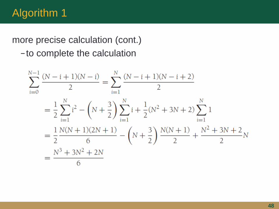
48
more precise calculation (cont.)
− to complete the calculation

Algorithm 2
49
to speed up the algorithm, we can remove a for loop
−unnecessary calculation removed
−note that
−new algorithm is 𝑂(𝑛2)

Algorithm 2
50

Algorithm 3
51
recursive algorithm runs even faster
−divide and conquer strategy
−divide: split problem into two roughly equal subproblems
−conquer: merge solutions to subproblems
−maximum subsequence can be in one of three places
−entirely in left half of input
−entirely in right half of input
− in both halves, crossing the middle
− first two cases solved recursively
− last case solved by finding the largest sum in the first half that includes the last element of the first half, plus the largest sum in the second half that includes the first element in the second half

Algorithm 3
52
consider the following example
−maximum subsequence for the first half: 6
−maximum subsequence for the second half: 8
−maximum subsequence that crosses the middle
−maximum subsequence in the first half that includes the
last element of the first half: 4
−maximum subsequence in the second half that includes
the first element in the second half: 7
−total: 11
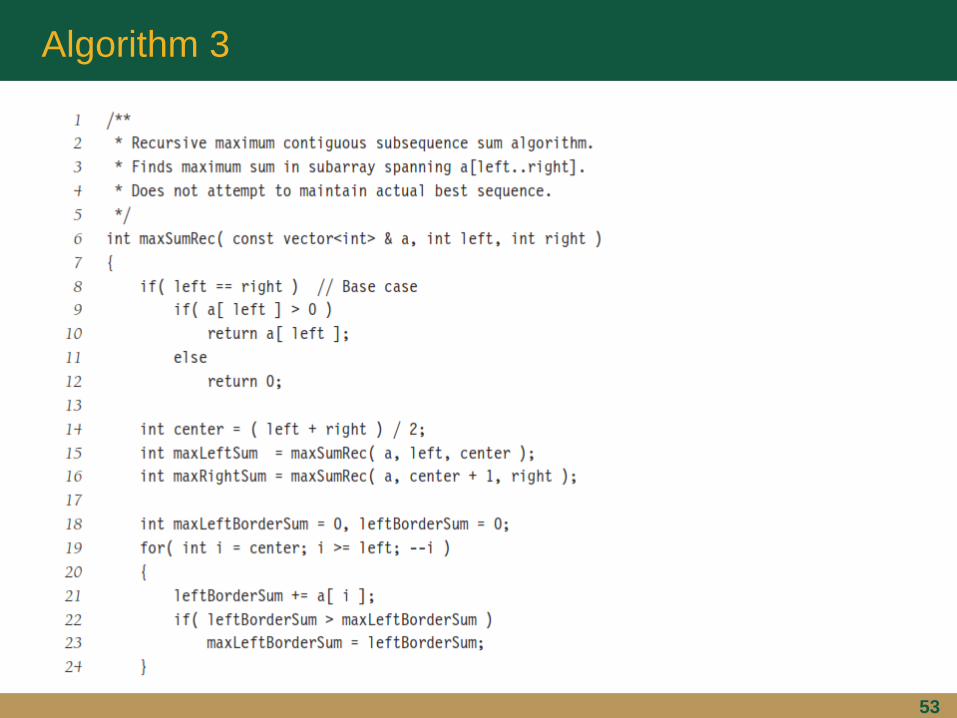
Algorithm 3
53

Algorithm 3 (cont.)
54

Algorithm 3
55
notes
−driver function needed
−gets solution started by calling function with initial
parameters that delimit entire array
− if left == right
−base case
− recursive calls to divide the list
−working toward base case
− lines 18-24 and 26-32 calculate max sums that touch the
center
−max3 returns the largest of three values

Algorithm 3
56
analysis
− let 𝑇(𝑁) be the time it takes to solve a maximum
subsequence problem of size 𝑁
− if 𝑁 = 1, program takes some constant time to execute
lines 8-12; thus 𝑇 1 = 1
−otherwise, the program must perform two recursive calls
− the two for loops access each element in the subarray,
with constant work; thus 𝑂(𝑁)
−all other non-recursive work in the function is constant
and can be ignored
− recursive calls divide the list into two 𝑁/2 subproblems if
𝑁 is even (and more strongly, a power of 2)
−time: 2𝑇(𝑁/2)
Algorithm 3
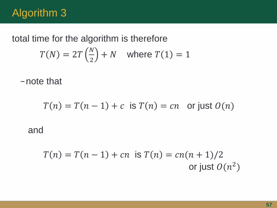
57
total time for the algorithm is therefore
𝑇 𝑁 = 2𝑇𝑁
2+ 𝑁 where 𝑇 1 = 1
−note that
𝑇 𝑛 = 𝑇 𝑛 − 1 + 𝑐 is 𝑇 𝑛 = 𝑐𝑛 or just 𝑂(𝑛)
and
𝑇 𝑛 = 𝑇 𝑛 − 1 + 𝑐𝑛 is 𝑇 𝑛 = 𝑐𝑛(𝑛 + 1)/2
or just 𝑂(𝑛2)

Algorithm 3
58
we can solve the recurrence relation directly (later)
𝑇 𝑁 = 2𝑇𝑁
2+ 𝑁 where 𝑇 1 = 1
− for now, note that
𝑇 1 = 1
𝑇 2 = 4 = 2 ∗ 2
𝑇 4 = 12 = 4 ∗ 3
𝑇 8 = 32 = 8 ∗ 4
𝑇 16 = 80 = 16 ∗ 5
thus, if 𝑁 = 2𝑘,
𝑇 𝑁 = 𝑁 ∗ 𝑘 + 1 = 𝑁 log𝑁 + 𝑁 = 𝑂(𝑁 log𝑁)

Algorithm 4
59
linear algorithm to solve the maximum subsequence sum
−observation: we never want a negative sum
−as before, remember the best sum we’ve encountered so
far, but add a running sum
− if the running sum becomes negative, reset the starting
point to the first positive element

Algorithm 4
60

Algorithm 4
61
notes
− if a[i] is negative, it cannot possibly be the first element of
a maximum sum, since any such subsequence would be
improved by beginning with a[i+1]
−similarly, any negative subsequence cannot possible be a
prefix for an optimal subsequence
−this allows us to advance through the original sequence
rapidly
−correctness may be difficult to determine
−can be tested on small input by running against more
inefficient brute-force programs
−additional advantage: data need only be read once (online
algorithm) – extremely advantageous

Logarithms in the Running Time
62
logarithms will show up regularly in analyzing algorithms
−we have already seen them in divide and conquer
strategies
−general rule: an algorithm is 𝑂(𝑁 log𝑁) if it takes constant
𝑂(1) time to cut the problem size by a fraction (typically 1
2)
− if constant time is required to merely reduce the problem
by a constant amount (say, smaller by 1), then the
algorithm is 𝑂(𝑁)
−only certain problems fall into the 𝑂(log𝑁) category
since it would take Ω(𝑁) just to read in the input
−for such problems, we assume the input is pre-read

Binary Search
63
binary search
−given an integer X and integers A0, A1, …, AN-1, which are
presorted and already in memory, find I such that Ai = X, or
return i = -1 if X is not in the input
−obvious solution: scan through the list from left to right to
find X
−runs in linear time
−does not take into account that elements are presorted
−better solution: check if X is in the middle element
− if yes, done
− if smaller, apply same strategy to sorted left subarray
− if greater, use right subarray

Binary Search
64

Binary Search
65
analysis
−all the work done inside the loop takes 𝑂(1) time per
iteration
− first iteration of the loop is for 𝑁 − 1
−subsequent iterations of the loop halve this amount
−total running time is therefore 𝑂(log𝑁)
−another example using sorted data for fast lookup
−periodic table of elements
−118 elements
−at most 8 accesses would be required

Euclid’s Algorithm
66
Euclid’s algorithm
−computes gcd (greatest common divisor) of two integers
− largest integer that divides both

Euclid’s Algorithm
67

Euclid’s Algorithm
68
notes
−algorithm computes gcd (M, N) assuming 𝑀 ≥ 𝑁
− if 𝑁 > 𝑀, the values are swapped
−algorithm works by continually computing remainders until
0 is reached
− the last non-0 remainder is the answer
− for example, if 𝑀 = 1,989 and 𝑁 = 1,590, the sequence of
remainders is 399, 393, 6, 3, 0
−therefore gcd = 3
−good, fast algorithm
Euclid’s Algorithm
69
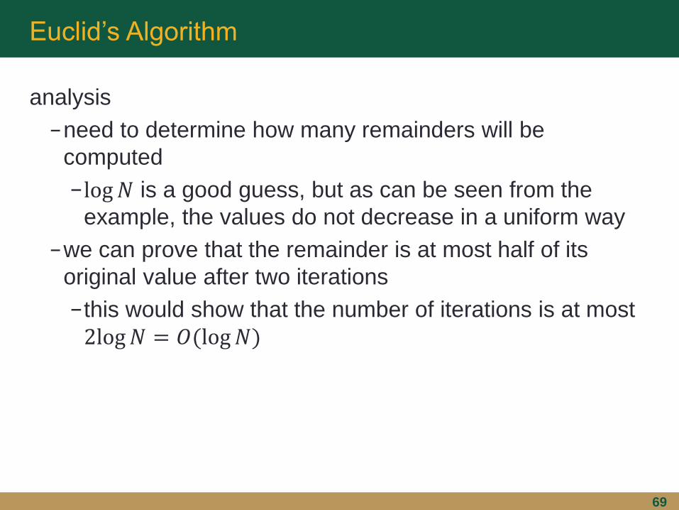
analysis
−need to determine how many remainders will be
computed
−log𝑁 is a good guess, but as can be seen from the
example, the values do not decrease in a uniform way
−we can prove that the remainder is at most half of its
original value after two iterations
−this would show that the number of iterations is at most
2log𝑁 = 𝑂(log𝑁)

Euclid’s Algorithm
70
analysis (cont.)
−Show: if 𝑀 > 𝑁, then 𝑁 < 𝑀/2
−Proof: 2 cases
− if 𝑁 ≤ 𝑀/2, then since the remainder is smaller than 𝑁,
the theorem is true
− if 𝑁 > 𝑀/2, then 𝑁 goes into 𝑀 once with a remainder
of 𝑀 −𝑁 < 𝑀/2, and the theorem is true
− in our example, 2log𝑁 is about 20, but we needed only 7
operations
−the constant can be refined to 1.44log𝑁
−the average case (complicated!) is
(12 ln 2 ln𝑁)/𝜋2 +1.47

Exponentiation
71
exponentiation
− raising an integer to an integer power
−results are often large, so machine must be able to
support such values
−number of multiplications is the measurement of work
−obvious algorithm: for 𝑋𝑁 uses 𝑁 − 1 multiplications
− recursive algorithm: better
−𝑁 ≤ 1 base case
−otherwise, if 𝑁 is even, 𝑋𝑁 = 𝑋𝑁/2 ∙ 𝑋𝑁/2
− if 𝑁 is odd, 𝑋𝑁 = 𝑋(𝑁−1)/2 ∙ 𝑋(𝑁−1)/2 ∙ 𝑋
−example: 𝑋62 = 𝑋31 2
𝑋3 = 𝑋2 𝑋, 𝑋7 = 𝑋3 2𝑋, 𝑋15 = 𝑋7 2𝑋, 𝑋31 = 𝑋15 2𝑋
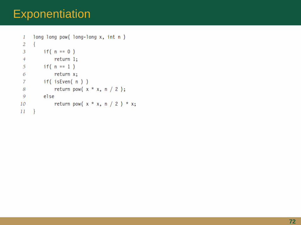
Exponentiation
72

Exponentiation
73
analysis
−number of multiplications: 2log𝑁
−at most, 2 multiplications are required to halve the
problem (if 𝑁 is odd)
−some additional modifications can be made, but care must
be taken to avoid errors and inefficiencies

Limitations of Worst-Case Analysis
74
analysis can be shown empirically to be an overestimate
−analysis can be tightened
−average running time may be significantly less than worst-
case running time
−often, the worst-case is achievable by very bad input,
but still a large overestimate in the average case
−unfortunately, average-case analysis is extremely
complex (and in many cases currently unsolved), so
worst-case is the best that we’ve got