Chapter 2

Investigation of Underwater Sound Wave Propagation Characteristics

and Development of Sonar Range Equation

2.1 Introduction

Navigation is the process of directing a vehicle from one known place to other known place.

All navigational techniques involve locating the position of the vehicle being navigated in

relation to the known datum. Tracking of the mobile object whether moving in terrestrial

environment or in underwater environment is very important activity towards fulfilling its

mission. The process of acquiring/identifying the location of an object of interest is called

positioning. The example of one of the best known positioning systems is the Global

Positioning System (GPS). In this chapter, various terrestrial navigation and global

positioning systems have been described along with various classical under water positioning

approaches. In the underwater environment, avoiding collision of the Autonomous

underwater vehicle (AUV) with floating or fixed objects requires either prior knowledge of

the operating environment or sensing equipment for evaluating the environment in real time.

Having prior knowledge is not feasible for unstructured environments and therefore having

the sensing equipment is the only viable option. The sensing equipment in this case is the

sonar that is mounted on the AUV which scans the area in front and provides the images as

the output. These images are then required to be processed in order to detect the objects

coming in the path of the AUV in order to have safe navigation. Navigation sensor is a device

used to measure a property from which the navigation system computes its navigation

solution (eg. radio navigation receiver). In the subsequent paragraphs investigation of

underwater sound wave propagation characteristics and development of sonar range equation

are presented.

2.2 Terrestrial Navigation

Navigation technique is a method of determining position and velocity of a vehicle. A

navigation system is also referred to as navigational aid. Navigational aid is a device that

determines position and velocity. Terrestrial navigation systems are radio positioning systems

that use land-based transmitters or reference points for the calculation of position

information. Some of the terrestrial based positioning systems which use techniques

developed during Second World War are still in use. They are long range aid to navigation

(LORAN), dead reckoning (DR), and inertial navigation systems (INS).

2.2.1 Dead Reckoning

Dead reckoning is the process of estimating present position by projecting course and speed

from a known past position. It is also used to predict the future position by projecting course

and speed from a known present position. Dead reckoning measures either the change in

position or the velocity and integrates it. This is added to the previous position in order to

obtain current position. The speed or distance tracked is measured in the body coordinate

frame, so a separate altitude measured is required to obtain the direction of travel in the

reference frame. For a 2D navigation, a heading measurement is sufficient, whereas for 3D

navigation, a full 3 component measurement is needed.

The navigator uses dead reckoning in many ways, such as:

to predict landfall, sighting lights and arrival times,

to determine sunrise and sunset,

to evaluate the accuracy of electronic positioning information,

to predict which celestial bodies will be available for future observation.

The most important use of dead reckoning is to project the position of the ship in the

immediate future and avoid navigation hazards. Usually these techniques are combined with

one or more position fixing techniques in an integrated navigation system to get the benefits

of both systems.

2.2.2 VOR (Very High Frequency Omnidirectional Range)

VOR provides azimuthal guidance to an aircraft. True bearing is determined from

comparison of the two signals (carrier mode reference phase signal and side band mode

variable phase signal). It operates in the 108 MHz-118 MHz frequency range. VOR transmits

an omnidirectional reference signal (30Hz AM signal) and a variable signal (30Hz FM signal

on a sub carrier) from rotating highly directional antennas. The phase of the variable signal is

electronically varied according to the absolute direction. The relative phase of the AM and

FM signals vary with azimuth. The VOR receivers can obtain their heading with respect to

magnetic north, from the VOR beacon to an accuracy of 1-20 which corresponds to 7-14 Km

position accuracy at maximum range. The user (eg. aircraft receiver) can calculate its heading

from the phase difference it is experiencing.

2.2.3 Inertial Navigation

Inertial navigation System (INS) is a 3D dead-reckoning navigation system. INS is also

known as Inertial Measurement Unit (IMU). It consists of inertial sensor called IMU and

navigation processor. The IMU comprises 3 mutually orthogonal accelerometers and 3

gyroscopes aligned with the accelerometers. The navigation processor integrates the IMU

outputs to give the position, velocity and the acceleration.

3 accelerometers

3 gyroscopes

IMU

Navigation Processor

Position,

Velocity and

Acceleration

Initial Conditions INS

Fig. 2.1 The basic components of an INS

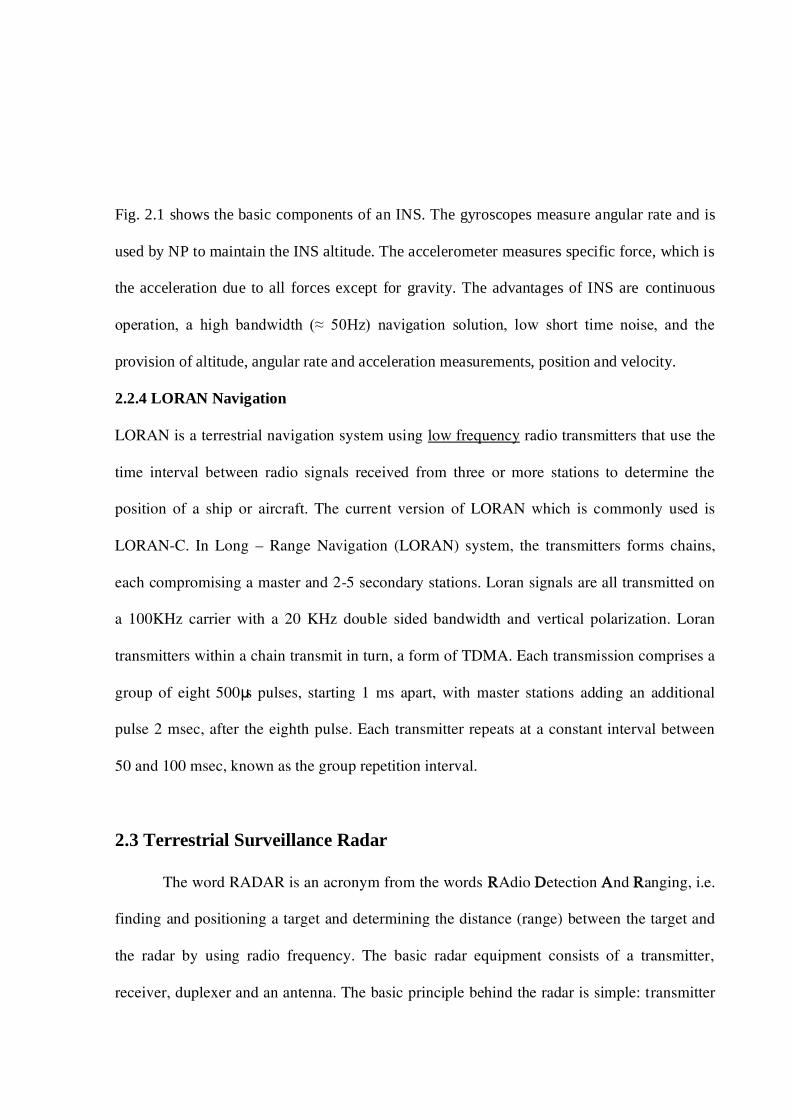
Fig. 2.1 shows the basic components of an INS. The gyroscopes measure angular rate and is

used by NP to maintain the INS altitude. The accelerometer measures specific force, which is

the acceleration due to all forces except for gravity. The advantages of INS are continuous

operation, a high bandwidth (≈ 50Hz) navigation solution, low short time noise, and the

provision of altitude, angular rate and acceleration measurements, position and velocity.

2.2.4 LORAN Navigation

LORAN is a terrestrial navigation system using low frequency radio transmitters that use the

time interval between radio signals received from three or more stations to determine the

position of a ship or aircraft. The current version of LORAN which is commonly used is

LORAN-C. In Long – Range Navigation (LORAN) system, the transmitters forms chains,

each compromising a master and 2-5 secondary stations. Loran signals are all transmitted on

a 100KHz carrier with a 20 KHz double sided bandwidth and vertical polarization. Loran

transmitters within a chain transmit in turn, a form of TDMA. Each transmission comprises a

group of eight 500μs pulses, starting 1 ms apart, with master stations adding an additional

pulse 2 msec, after the eighth pulse. Each transmitter repeats at a constant interval between

50 and 100 msec, known as the group repetition interval.

2.3 Terrestrial Surveillance Radar

The word RADAR is an acronym from the words RAdio Detection And Ranging, i.e.

finding and positioning a target and determining the distance (range) between the target and

the radar by using radio frequency. The basic radar equipment consists of a transmitter,

receiver, duplexer and an antenna. The basic principle behind the radar is simple: transmitter

sends out a very short duration pulse at a high power level. The pulse strikes an object (or a

target) and energy will be reflected (known as radar returns or echoes) back to the radar

receiver. Radar determines the distance (range) to the target by measuring the travel time of

the radar pulse to get the target and to come back and then divides that time in two.

For extracting the target information from the echo, the signal must be of sufficient

magnitude. The radar equation is used to predict the echo power to assist in making the

determination of whether or not above mentioned condition is met. These echoes are then

processed by the radar receiver to extract target information such as range, velocity, angular

position, and other target identifying characteristics. Radar can perform its function at long or

short distances and it can operate in darkness, haze, fog, rain, and snow. Its ability to measure

distance with high accuracy and in all weather conditions is one of its most important

attributes.

Radar Range Equation

The radar equation provides the relationship between the transmitted power, the

received power, the characteristics of the target, and characteristics of the radar itself. The

equation is also helpful to assess the performance of the radar. The maximum radar range

Rmax is given by

4/1

min3

22

max)4( S

GPR t

(2.1)

Where, Rmax is the maximum detection range between the radar and the target. It has the units

of meters (m).

Pt is termed the peak transmit power and is the average power when the radar is

transmitting a signal. It has the units of Watts.

λ is the radar wavelength. It has the units of meters (m).

G is the gain of the transmitter and receiver antenna.

σ is the target radar cross section or RCS and has the units of meters or m2.

Smin the minimum received power that the radar receiver can ‘sense’ and is referred

to as Minimum Detectable Signal (MDS). It has the units of Watts.

Properties of reflection of electromagnetic waves:

1. Electromagnetic energy travels through air at a constant speed, at approximately the

speed of light,

300,000 kilometres per second or

186,000 statute miles per second or

162,000 nautical miles per second.

This constant speed allows the determination of the distance between the reflecting

objects (airplanes, ships or cars) and the radar site by measuring the running time of

the transmitted pulses.

2. This energy normally travels through space in a straight line, and will vary only

slightly because of atmospheric and weather conditions. By use of special radar

antennas this energy can be focused into a desired direction. Thus the direction (in

azimuth and elevation) of the reflecting objects can be measured.

These principles can basically be implemented in a radar system, and allow the determination

of the distance, the direction and the height of the reflecting object.

2.4 Satellite Based Navigation Systems

Modern navigation systems are of two types. They are ground based and satellite

based navigation systems. Various ground based navigational systems are VOR, ILS,

LORAN etc. The ground based navigation systems encounter the problems such as ground

reflections, electromagnetic interference and reflections from the physical entities. These

problems are mostly nil in satellite based navigation systems, due to the space constellation.

Satellite navigation is based on a global network of satellites that transmit radio signals in the

low/medium earth orbit. The satellite navigation system has the following advantages: (i) The

satellite can transmit a radio frequency and carry a transponder beacon which provides all

weather service (ii) satellite navigation systems are capable of high accuracy. The modern

satellite based navigation systems are: TRANSIT, GPS, GLONASS and GALILEO.

2.4.1 TRANSIT

Transit was the first satellite aided navigation system deployed for civilian use from

1967. Transit worked on the Doppler principle using seven low orbiting satellites. Each of

these satellites used to transmit on two frequencies i.e., 150MHz and 400MHz. Position was

calculated by measuring the change in frequency of the satellite transmissions as it used to

speed past in low orbit. Using the satellite’s position and velocity information, the user

position was calculated by measuring the change in frequency of the satellite transmissions.

The TRANSIT satellites were orbiting in polar plane at an altitude of about 1100Km. The

TRANSIT satellites were affected more by gravity field variations than the higher orbiting

satellites like GPS. Since their numbers were limited, one did not get a ‘fix’ very often.

Further, transmissions of TRANSIT satellites at 150MHz and 400MHz were more

susceptible to ionospheric delays and disturbances than the higher Global Positioning System

(GPS) frequencies. After GPS became fully operational, TRANSIT was discontinued on 31st

December 1996 (Leick, 2004).

Several orbiting satellite systems, which are presently used for global positioning, include:

United States Global Positioning System (GPS)

Russian Global Navigation Satellite System (GLONASS)

European Galileo system

2.4.2 GPS

GPS is a satellite based radio navigation system designed and developed by the

Department of Defense (DOD), U.S.A. The first GPS satellite was launched on February 22,

1978. GPS provides accurate three dimensional user position anywhere in the world and

under all weather conditions (Kaplan 1996). The satellites transmit at frequencies L1

(1575.42MHz) and L2 (1227.6MHz) modulated by the two types of codes and the navigation

message. At present the L1 carrier is modulated with C/A and P-codes, whereas L2 is

modulated with P-code only. The advantages of GPS are: i) intentional interference like

Jamming and unintentional interference will affect GPS least since spread spectrum

techniques are used in it and ii) system accuracy can be improved to the order of centimeters

using differential techniques like Differential Global Positioning System (DGPS), WAAS,

GAGAN etc., Full operational capability of GPS was achieved on July 17, 1995.

i) Principle of operation of GPS: GPS is operating on a set of 24 satellites that are

continuously orbiting the earth. These satellites are equipped with atomic clocks and send out

radio signals as to the exact time and their location. The radio signals from the satellites are

picked up by the GPS receiver. Once the GPS receiver locks on to four or more of these

satellites, it can triangulate its location from the known positions of the satellites.

ii) Basic equations for finding user position

In this section, the basic equations for determining the user position are presented. Assume

that the distance measured is accurate and under this condition, three satellites are sufficient.

In Fig. 2.2, there are three known points at locations r1 or (x1, y1, z1), r2 or (x2, y2, z2), and r3

or (x3, y3, z3), and an unknown point at ruor (xu, yu, zu). If the distances between the three

known points to the unknown point can be measured as ρ1, ρ2, and ρ3, these distances can be

written as

(2.2)

(2.3)

(2.4)

Because there are three unknowns and three equations, the values of xu, yu, and zu can be

obtained from these equations. Theoretically, there should be two sets of solutions as they are

second-order equations. These equations can be solved easily with linearization and an

iterative approach. In GPS operation, the satellite positions information can be obtained from

the data transmitted from the satellites.

Fig. 2.2 Use of three known positions to find one unknown position.

The distances from the user (the unknown position) to the satellites must be measured

r1(x1,y1,z1) r2(x2,y2,z2)

r3(x3,y3,z3)

(xu,yu,zu)

user location

x

y

z

ρ1

ρ2

ρ3

simultaneously at a certain time instant. Each satellite transmits a signal with a time reference

associated with it. By measuring the time of the signal travelling from the satellite to the user,

the distance between the user and the satellite can be found (G S Rao, 2010).

2.5 Underwater Navigation

Under water navigation is the process of directing the movements of submersible vehicles,

including divers, from one point to another. The development of contemporary submersible

vehicles, coupled with advances in saturated diving, has resulted in new requirements for

underwater navigation. The choice of the navigation system therefore depends on factors like

required precision, area to be covered, availability of surface vessels, sea state under which

they are expected to operate, including the redundancy which is necessary for safety.

Submarines are required to operate over wide areas of the ocean and often under highly

secure and covert conditions; therefore, navigation techniques which depend upon acoustics

are needed because the techniques like Radar and GPS cannot be used. This is because radar

uses radio waves in the microwave frequency range, which have approximately one

centimetre wavelength. This wavelength range is used because it is easier to direct the waves

with small antennas in narrow beams. Unfortunately, microwaves are strongly absorbed by

sea water within very short distance of their transmission. The reason is mainly because sea

water is good conductor of electricity. Therefore to detect the target which is at a distance of

miles away, it is not possible to use radar in underwater environment.

Similarly GPS is also unusable for underwater navigation because the signal used in GPS is

also an electromagnetic signal, which propagates well in air but can only travel for a very

short distance underwater because of its high absorption rate in water. Seventy percent of the

Earth is covered by sea. In these areas where Radar and GPS cannot work, alternative

underwater positioning systems play an important role. Positioning an underwater target with

respect to a reference platform is required in diverse areas in ocean scientific research,

industry engineering tasks and military activities. An underwater acoustic positioning system

tracks and navigates underwater vehicles or divers by means of acoustic distance and

direction measurements, and subsequent position triangulation. Unlike the in-land positioning

systems such as GPS, which use electromagnetic signals, the underwater positioning systems

use acoustic signals, because acoustic signals have a lower absorption rate in sea water, as

compared to that of electromagnetic signals. As a result, acoustic wave can propagate a much

longer distance in underwater environment. Basic components of an acoustic positioning

system include a transceiver and an array of transponders (or a transponder and an array of

transceivers), a processing unit and a display unit. The transceivers and the transponders

transmit and receive acoustic signals for distance and direction measurements. The spacing

between transponders (or transceivers) in the array is called baseline. Underwater acoustic

positioning systems are categorized into three major groups according to the size of their

baselines as

i) Long Baseline (LBL) Systems

ii) Short Baseline (SBL) Systems

iii) Ultra-Short Baseline (USBL) Systems

In addition, also due to fast development in GPS technology, new underwater acoustic

positioning systems have arisen that utilize buoys equipped with GPS receivers and acoustic

communication techniques.

2.5.1 Long Baseline (LBL) Positioning Systems

A typical LBL positioning system consists of one transceiver and at least three transponders.

The transceiver is mounted on a submersible or a surface vessel, which is the target to be

positioned. The transponders are installed on the seafloor to form an array. Before positioning

the target, transponders will be deployed on the seafloor. Their position (or at least the

distances between each other) needs to be known precisely. The deployment and retrieval of

transponders on the seafloor is performed by a surface ship, or by divers or an underwater

automatic vehicle. The spacing between transponders (i.e. the LBL baseline) is 50-2000m in

an LBL system. The transceiver on the target pings each transponder on the seafloor. The

travelling time of the transmitted signal from the target to the transponders and backwards is

measured. Knowing the sound velocity at the site allows this measurement to be converted

directly in to travelling distances. Once the distances from all transponders to the transceiver

are obtained, a unique point where all these distances intersect is obtained via calculations

and this point is the position of the transceiver. This method is called “trilateration”. The

calculated transceiver’s position is within and referenced to the transponders array. Fig. 2.3

illustrates the Long Baseline Positioning Systems.

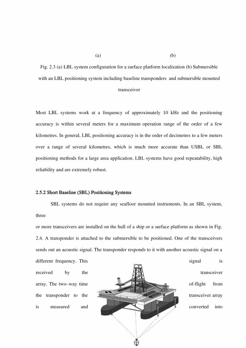
(a) (b)

Fig. 2.3 (a) LBL system configuration for a surface platform localization (b) Submersible

with an LBL positioning system including baseline transponders and submersible mounted

transceiver

Most LBL systems work at a frequency of approximately 10 kHz and the positioning

accuracy is within several meters for a maximum operation range of the order of a few

kilometres. In general, LBL positioning accuracy is in the order of decimetres to a few meters

over a range of several kilometres, which is much more accurate than USBL or SBL

positioning methods for a large area application. LBL systems have good repeatability, high

reliability and are extremely robust.

2.5.2 Short Baseline (SBL) Positioning Systems

SBL systems do not require any seafloor mounted instruments. In an SBL system,

three

or more transceivers are installed on the hull of a ship or a surface platform as shown in Fig.

2.4. A transponder is attached to the submersible to be positioned. One of the transceivers

sends out an acoustic signal. The transponder responds to it with another acoustic signal on a

different frequency. This signal is

received by the transceiver

array. The two–way time of-flight from

the transponder to the transceiver array

is measured and converted into

slant range if the sound speed at the site is known. The submersible’s position is obtained by

using the trilateration method. The SBL positioning accuracy improves with the operating

range and the spacing between the transceivers on the surface platform. Thus, where space

permits, such as when operating from larger vessels or a dock, the SBL system can achieve a

precision and position robustness that is similar to that of seafloor mounted LBL systems,

making the system suitable for high-accuracy survey work.

Fig. 2.4 SBL positioning system

As compared to LBL systems, the low system complexity makes SBL easy to use. It is a ship

based system so there is no need to deploy transponders on the seafloor, which saves time

and money. SBL systems are mainly used to track a submersible with respect to a surface

platform such as an oil drilling platform. SBL system also can be used for searching a

crashed airplane in the sea.

2.5.3 Ultra Short Baseline (USBL) Positioning Systems

Ultra Short Base Line system (USBL) is sometimes called Super Short Base Line

(SSBL) system. Similar to the SBL system, an array of transceivers (three or more) is fixed to

a surface vessel. A transponder is attached to a submerged target, which could be an ROV, an

AUV, a crawler or a diver as shown in Fig. 2.5. An acoustic pulse is transmitted by the

transceiver and detected by the transponder on the target, which replies with its own acoustic

pulse. This return pulse is detected by the shipboard transceivers array. The time from the

transmission of the initial acoustic pulse until the reply is detected is measured and converted

into a range. Instead of using the trilateration to calculate a subsea position, the USBL

measures both the range and the angle from the subsea target to the transceiver array. The

distance from the transceiver to the target, r, is the amplitude of the target vector. It is

obtained by measuring the time of arrival, as in LBL and SBL systems. The Cartesian

coordinates (x, y, z) of the target (Fig 2.6) are given by:

cossinrx

(2.5)

sinsinry

(2.6)

cosry

(2.7)

Fig. 2.5 USBL positioning system

z

Fig. 2.6 USBL range and angle measurements

The transceivers in a USBL system are typically built into a single assembly in close

proximity, which makes USBL systems more compatible and easy to deploy. It has better

performance within short range or in shallow water. The positioning performance depends on

the accuracy of additional sensors for vessel self-motions.

2.5.4 Common Issues Associated with Acoustic Positioning Systems

The major problems associated with the commercially available underwater acoustic

positioning systems include positioning accuracy, system complexity and cost. Acoustic

positioning systems can yield an accuracy of a few centimetres to tens of meters and can be

used over operating distances of tens of meters to tens of kilometres. Performance depends

strongly on the type and model of the positioning system, its configuration for a particular

job, and the characteristics of the underwater acoustic environment at the work site. Factors

that reduce the system performance include sound velocity variations, noise, multipath, and

the inhomogeneities of the sea water. The sound speed in water is a function of water

temperature, salinity and depth and the variations in sound speed will bring a systematic

error. The sound speed must be monitored in different areas and at different times throughout

the positioning task within the required accuracy of the survey to maintain the positioning

accuracy. Another factor that reduces the positioning accuracy in underwater is the multipath

interferences.

The conventional systems usually involve a surface ship and multiple transducers.

This type of configuration is not economic for long term observations of underwater activities

such as the monitoring of the marine habitat at a certain spot. The costs of individual

equipments, plus the expense on system components deployment in each of the research trial,

should also be taken into account. The absolute position of the target depends on additional

sensors like sonar.

2.6 Autonomous Underwater vehicle (AUV)

An Autonomous Underwater Vehicle (AUV) is a robot which travels underwater

without requiring input from an operator. In military applications AUVs are often referred to

as unmanned undersea vehicles (UUVs).

Once an AUV is deployed it drives around by gathering different kinds of sensor

measurements. In order to make any sense of these measurements, the AUV has to be able to

keep a track of where the measurements were made. Also to make a successful survey it is

necessary to be able to direct the vehicle to a particular location and keep track of where it

has been with respect to the earth’s axis so that the data gathered by the AUV can be

associated to a particular X-Y location. This issue is a little easier to deal with using high

quality sensor maps of the area apriori.

This leads to the next type of navigation, which involves building a map starting from a

known point, while using it to navigate and at the same time updating the map using the new

sensor data available. In the underwater environment the navigation problem is further

complicated by the fact that EM waves attenuate very quickly. Even in optimal conditions the

optical data would be limited to a few meters.

The traditional methods for navigation are underwater acoustic positioning systems. The LBL

setup under optimal condition can provide highly accurate position fixes for the AUV which

means it can accurately keep a track of the AUV during the survey. The limitation of the LBL

navigation is that acoustic waves have a significant travel time in water which means that the

frequency of the LBL fixes is highly limited .Also another problem with these systems are the

false returns received by the transducers when the acoustic waves bounce off the surface,

seafloor or other reflecting thermal layers. Even though LBL systems can be very efficient

for doing detailed surveys of a small area, it requires a lot of ship time to setup and deploy

which makes it inconvenient and expensive for large area surveys. Similarly the USBL

systems can be used with a reasonable level of accuracy, but nowhere near to that of the LBL

systems. Other disadvantages of the USBL system are that they need to be calibrated well to

get a reasonable accuracy and the USBL system relies on data from other sensors like the

gyro and depth sensor to get a reliable absolute positioning. Though USBL systems are not

very accurate on their own, they can be used along with dead reckoning to provide reasonably

high accuracy. Thus, the USBL systems can be used for basic navigation of the AUV, but do

not meet the requirements for the high accuracy needs of the surveying AUVs. All the above

discussed methods do not meet the requirements for the high accuracy needs of the surveying

AUVs which leads to searching for another source energy for underwater navigation.

The choice of energy to be used for underwater detection is determined by three factors:

i) Range of penetration in the medium.

ii) Ability to differentiate between various objects in the medium.

iii) Speed of propagation.

Of all the known physical phenomena, light has excellent differentiation ability and high

speed of transmission, but its range in water is very limited, on the order of tens of meters,

thereby restricting its operational usefulness. Radio frequency waves also can propagate with

extreme rapidity and to larger distances through space or transmission medium, but sea water

is essentially impervious to them for most frequencies. VLF signals will penetrate only about

10 meters therefore it is insufficient for normal surveillance whereas acoustic energy is

capable of being transmitted through the sea to larger distances that are operationally

significant. Because of this, sound/ underwater energy is used for antisubmarine warfare,

underwater communications, and underwater navigation. The acoustic energy too has

significant limitations and they must be thoroughly understood by the operators of

underwater sound equipment. The optimum use of sound requires a thorough understanding

of its limitations so that these effects can be minimized. For example, sea water is not

uniform in terms of pressure, temperature, and salinity and all these characteristics have

important effects on sound propagation through the sea.

Avoiding collision of the AUV with the floating or fixed objects in the underwater scenario

needs either prior knowledge of the operating environment or sensing equipment for

evaluating the environment in real time. Having prior knowledge is not feasible for

unstructured environments and therefore sensing equipment must be used for executing the

second approach. AUVs carry sensors to navigate autonomously and map features of the

ocean. There are a few sensors that are available to overcome these issues. Sonar is a

sensor/technique that uses sound propagation, mounted onto the AUVs to navigate,

communicate with or detect underwater mines (Meyroqitz A. L. et al, 1996; Dong-Hoon

Yang, 2006).

2.7 Sonar Operating Principle

Sonar refers to the application of sound for the detection and location of underwater

objects. Sonar is the most successful method used for detecting the presence of objects

underwater. The simplest sonar devices send out a sound pulse from a transducer and then

precisely measure the time it takes for the sound pulses to reflect back to the transducer. The

distance to an object can be calculated using this time difference and the speed of sound in

the medium. This principle of operation of the sonar is shown in Fig. 2.7.

Fig. 2.7 Principle of operation of sonar

There are two types of the sonar: passive sonar and active sonar.

Passive Sonar

Passive sonar is a listening device; the sound waves produced by another source such

as ships, biological creatures or due to seismic activities are received by the sonar’s receiver

and changed into electrical signals for analysis and also for display on a monitor. Since the

frequencies emitted by the various sources are different, it is sufficient to receive these

frequencies in order to identify the source. The direction of the source can also be found out

either by beam forming method or through the triangulation method by having the

measurements at different places. This will not be dealt here in detail as the aim of the

research is related to the imaging sonars which are active.

Active Sonar

Active sonar is the one which sends the signals and receives the echo. Active sonar

uses a transducer which converts electrical signal to sound waves. These sound waves are

reflected back from the target and detected by the sonar’s receiver as an echo. The receiver

passes sound waves to the transducer which converts the sound back to electrical signals.

Since the speed of the sound in water is known, the range and the bearing of the target can be

determined. This method is also known as echo-ranging. The block diagram of active sonar is

shown in Fig. 2.8.

Fig. 2.8 Block diagram of active sonar

2.8 Sound Propagation in Underwater Medium

The basic theory of acoustics involves the study of vibration, waves and their

propagation. If the direction of particle vibration is the same as the direction of wave

propagation, then the wave is called a longitudinal wave. If the direction of particle vibration

Target

Echo

Transmitted

Sound wave

time

Transducers

Vibration

Voltage

Oscillation

TRANSDUCER

TRANSMITTER RECEIVER

Display

is perpendicular to the direction of wave propagation, then the wave is called a transversal

wave. When a sound wave propagates in sea water, the structure of the water medium is

changed, resulting in the spread of sound energy. The sensing of an underwater receiver for

sound pressure is based on this sound pressure change. In the wave propagation process,

particles in the sea water do not move from one place to another, but only vibrate around

some fixed point. The acceleration speed of a particle is always proportional to the distance

from a fixed point. This kind of motion is called resonance motion. It is the simplest form of

periodic motion (Qihu Li., 2012). The expression of a one-dimensional differential equation

of resonance motion is

02

2

2

xwdt

xd

(2.8)

The solution of this equation is

x(t) = A sin(ωt) + B cos( ωt)

(2.9)

Where A, B are arbitrary constants and ω=2πf is the cycle frequency with unit rad/s, and the

unit of f is Hz.

2.8.1 Velocity of sound wave

Sound travels more slowly in fresh water than in sea water. The speed of sound is determined

by the water's bulk modulus and mass density. The bulk modulus is affected by temperature,

dissolved impurities (usually salinity), and pressure. The density effect is small. The speed of

sound (in feet per second) is approximately:

4388 + (11.25 × temperature (in °F)) + (0.0182 × depth (in feet)) + salinity (in parts-per-

thousand)

This empirically derived approximation equation is reasonably accurate for normal

temperatures, concentrations of salinity and the range of most ocean depths. Ocean

temperature varies with depth, but at between 30 and 100 meters there is often a marked

change, called the thermocline, dividing the warmer surface water from the cold, still waters

that make up the rest of the ocean. The sonar may not produce the desired result as the sound

originating on one side of the thermocline tends to be bent, or refracted, through the

thermocline. The thermocline may be present in shallower coastal waters. However, wave

action will often mix the water column and eliminate the thermocline. Water pressure also

affects sound propagation: higher pressure increases the sound speed, which causes the sound

waves to refract away from the area of higher sound speed. The mathematical model of

refraction is called Snell's law.

The propagation velocity c of sound in the sea can be derived from the following adiabatic

equation

aK

pc

1

(2.10)

where, p is the sound pressure, ρ is the density of water, and Ka is the adiabatic compression

coefficient. In sea water, since pKa is a function of temperature, salinity and pressure, the

sound speed in sea water is also a function of temperature, salinity and pressure, but

temperature is the dominant factor. In fresh water, the empirical formula for calculating

sound speed is generally

c=1410+4.21t-0.037t2+0.018d (m/s)

(2.11)

where, t is the temperature of sea water in 0C; d is the depth (m). c ≈1,500 m/s, for t = 20

0C.

The empirical formula for calculating sound speed in sea water is given by

c=1410+4.21t-0.037t2+1.1S+ 0.018 d(m/s)

(2.12)

where S is the salinity (%). C ≈1,500 m/ s when t = 14°C, S = 34.5, d = 15m.

Because the propagation characteristics of sound in the sea strongly depend on the

sound speed, it is very important to understand the distribution of sound speed for any

specific area. The relation between sound speed and depth is called the sound speed profile

(SSP). The SSP is related to the latitude, season, and day /night.

2.8.2 Sound pressure and sound power

"Sound power" and "Sound pressure" are two distinct and commonly confused

characteristics of sound. Sound power or acoustic power is a measure of the total sound

power emitted by a source in all directions in watts (joules per second) per unit time t. Sound

power levels are connected to the sound source and are independent of distance. Sound power

levels are indicated in decibel as follows

o

wI

IL 10log10

(2.13)

where sound power Io is chosen to be a reference sound power, define it as 0 dB, and then

any other sound power I has the dB value of 20log I/Io dB with respect to reference level.

Sound pressure is a pressure disturbance in the air whose intensity is influenced not only by

the strength of the source, but also by the surroundings and the distance from the source to

the receiver and diminishes as a result of intervening obstacles and barriers, air absorption,

wind and other factors. Sound pressure levels quantify in decibels and the intensity of given

sound sources are indicated in decibels.

Sound pressure level (SPL) o

pP

PL 10log10

(2.14)

Where sound pressure Po is chosen to be a reference sound pressure, define it as 0 dB, and

then any other sound pressure P has the dB value of 20log P/Po dB.

A frequently used method of estimating the sound power level at a source Lwis to measure the

sound pressure level Lp at some distance r, and solve for Lw. If the source is in free space

2104

1log10

rLL pw

(2.15)

or if the source is on the floor or on a wall, such that it radiates into a half sphere.

2104

2log10

rLL pw

(2.16)

2.8.3 Transmission loss of sound in underwater

Transmission Loss is the parameter that compares the amount of intensity of the signal at a

specific range from the source to the source intensity at one yard. The equation for this would

be:

)(

)1(log10

rI

ydITL

(2.17)

In sonar equations, transmission loss TL is an important parameter in sonar design because

the performance of a sonar system depends only on the transmission loss. When a sound

wave propagates in an ocean environment, the sound intensity will gradually decrease with

travel distance, because of the following reasons:

i) The geometrical spread of the wave front, spherical or cylindrical spreading,

ii) The loss of the sound wave at the sea surface and the sea floor,

iii) Sound absorption,

iv) Sound reflection.

Spreading and Cylindrical Losses

Sound waves while propagating underwater they get attenuated due to cylindrical and

spherical spreading of the energy. Cylindrical spreading presents underwater only when the

sea surface and the sea floor are flat. However spherical spreading presents underwater in all

kinds of sea environment. The transmission loss increases linearly in both spherical and

cylindrical spreading and the transmission loss due to spherical spreading is twice the

transmission loss due to cylindrical spreading.

2.8.3.1 Spreading Loss

Let’s assume a point source which emits a signal in all directions (that is in three

dimensions). The source would produce wave fronts that were spheres that would grow in

size as the wave propagates away from the source as shown in Fig 2.9.

Fig. 2.9 Spherical spread

rTL log20

(2.18)

The above equation is for transmission loss only due to spherical spreading. In this case, from

1 m to 100 m, the intensity of the sound wave will attenuate by 40 dB. Spherical spreading is

the most dominant factor in the transmission loss portion of the passive sonar equation. As

the range increases the transmission loss increases linearly as shown in Fig 2.10 and the

corresponding values are given in Table 2.1.

4 R2

R

10-3

10-2

10-1

-140

-130

-120

-110

-100

-90

-80

-70

-60

-50

-40

Range(km)

transm

issio

nlo

ss(d

B)

Fig. 2.10 Typical transmission loss curve of band limited signal

Table 2.1 Range prediction by calculation

of transmission loss for spherical spread

2.8.3.2 Cylindrical Spreading

In the propagation of a sound wave, if the sea

surface and sea floor are relatively flat, sound

reflection and absorption are negligible, so the

spread of a sound wave can be considered as cylindrical (Fig. 2.11). The transmission loss is

proportional to the distance R. As the range increases the transmission loss increases linearly

as shown in Fig 2.12 and the corresponding values are given in Table 2.2.

Range(m) Transmission loss(dB)

1 -138.1

5 -105.9

10 -92.1

20 -78.2

50 -59.9

70 -53.1

100 -46.0

10-1

100

101

102

-100

-90

-80

-70

-60

-50

-40

-30

-20

. The transmission loss due to cylindrical spreading is half of the spherical spreading.

Fig 2.11 Cylindrical spread

TL(R) = 101ogR

(2.19)

Fig. 2.12 Typical transmission loss curve of band limited signal

Range(m) Transmission loss(dB)

1 -69.0

5 -52.9

10 -46.0

20 -39.1

50 -29.9

70 -26.5

2 R2

R

h

Source

Range (km)

Tra

nsm

issi

on

lo

ss (

dB

)

100 -23.0

Table 2.2 Range prediction by calculation of transmission loss for cylindrical spread

The only limitation of this equation is that it does not take into account the spreading of the

wave spherically until it reaches the “transition range” where the wave starts to spread

cylindrically.

2.8.4 Sound absorption in underwater

Sound absorption in sea water is one of the important characteristics of an acoustic

channel. This is because, as the information carrier, in the propagation of a sound wave,

energy dissipation is the main characteristic of a channel. Sea water is not an ideal medium

for sound transmission. The absorption of sound in seawater forms part of the total

transmission loss of sound from a source to a receiver. It depends on the seawater properties,

such as temperature, salinity and acidity as well as the frequency of the sound. Absorption is

the conversion of acoustic energy to heat in the fluid. There are three main causes of

absorption losses:

i. Viscosity

ii. Change in molecular structure

iii. Heat conduction

Attenuation losses in sea water occur from both sound absorption losses and scattering losses.

This attenuation causes a decrease in the amplitude of the wave and an exponential decrease

in the acoustics pressure resulting in more spreading loss. To account for attenuation in the

transmission loss equation, a new term, α must be defined, the attenuation coefficient. Using

this new term, the transmission loss can be calculated using the equation:

dBydrTL nattenuatio

310))1((

(2.20)

where r is in yards. Generally, since the range, r, is usually much greater than 1 yard, we can

ignore the -1yard term in the equation. Thus the transmission loss can be expressed as:

dBrTL nattenuatio )10( 3

(2.21)

The most difficult problem in the transmission loss is to determine a correct value for α, i.e.,

the attenuation coefficient and the various factors that affect the attenuation coefficient are

given below.

i) Viscosity

The viscosity losses are due to two distinct effects. Each of these effects is dependent on not

only how the molecules act together in the medium as defined by the coefficients of both

shear and volume viscosity but also the frequency of the sound waves.

When both terms are combined and nominal values used for the density, speed of

sound and the coefficients, the value for the attenuation coefficient becomes

241075.2 f

(2.22)

where f is the sound wave frequency in kHz.

ii) Ionic Relaxation

The below equation describes how Ionic Relaxation affects the attenuation coefficient is

24

4100

40

f

fMgSO

(2.23)

where frequency, f, is in kHz.

Though many factors affect this complex process, simply suffice it to say that an equation for

this process’ affect on α would be

2

2

1

1.0

f

fborateboron

(2.24)

iii) A non-absorption factor, scattering

The last factor that contributes to losses is the scattering of sound energy due to in

homogeneities in seawater. This factor can be approximate as a constant, not dependant on

frequency and would only be a dominant factor below 100 Hz or so. This can be expressed as

kyddBscattering /003.0

(2.25)

When all these factors are combined, the equation for transmission loss then becomes:

dBrTL )10( 3

(2.26)

where

24

2

2

2

2

1075.24100

40

1

1.0003.0 f

f

f

f

fdB/kyd

(2.27)

The unit dB / ky can be converted to dB / km by multiplying with a factor of 1.094 then

absorption coefficient can be written as

)/(094.1 0 kmdB

(2.28)

The characteristics of absorption of sound in water is shown in Fig. 2.13 and corresponding

values are given in Table 2.3

Fig. 2.13 Absorption of sound in sea water

Table 2.3 Variation of absorption coefficient with frequency

2.9 Description of terms used in Sonar equations

The sonar equation is based on a basic equality between the desired and undesired

parts of the received signal at the instant the desired function of the sonar has been achieved.

These functions could be detection of an underwater target or detection of any other source

produced by the acoustic activities. These functions involve the reception of the acoustic

signals occurring in a natural acoustic noise background. Of the combined received acoustic

signal at the receiver, the desired portion is called the signal and the rest is called noise which

Frequency(kHz) Absorption coefficient(dB)

0.1 1.1114e-004

0.5 0.0025

1.0 0.0086

2.0 0.0217

3.0 0.0302

4.0 0.0349

is undesired. In sonar the background is either noise, which is essentially a portion not due to

one’s own sonar, or reverberation, the slowly delayed portion of the background representing

the return of one’s own acoustic output by scatters in the medium. For better performance of

the sonar, the overall response of the system to the signal is increased and its response to the

background is decreased. A signal is said to be detected when its level equals the level of the

background noise.

Signal level = background noise level

The equality mentioned exists only at one instant in time, as the target approaches or recedes

from the sonar receiver. At short ranges, its signal will exceed the background noise level but

at long ranges, the reverse will occur. The basic equations can be expanded in term of various

parameters. These parameters are attributed to the equipment, the medium, and the target.

These parameters are expressed in terms of decibel. These are expressed as follows:

The Equipment

Projector Source Level: SL

Self-Noise Level: NL

Receiving Directivity Index: DI

Detection Threshold: DT

The Medium

Transmission Loss: TL

Reverberation Level: RL

Ambient-Noise Level: NL

The Target

Target Strength: TS

Target Source Level: SL

In subsequent paragraphs these are explained in further detail.

i) Projector Source Level (SL)

Source level is defined differently for active and passive sonar equations. For the

active sonar equations, it is the sound pressure level of the actively transmitting sonar,

measured (or referenced to) one yard from the transducer. For the passive sonar equation, the

source level is the measure of the noise generated by the object at specific frequencies and is

also referenced to one yard from the sound source.

ii) Receiving Directivity Index (DI)

Directivity index indicates the amount by which sonar uses its directional beam

forming capability by discriminating omni directional noise from a directional signal. The

directivity index is a function of the sonar's design and the received frequency only.

Directivity index is the measure of the amount by which a given sonar system can filter out

background noise by using its directional beam forming capability. The value for the

directivity index for a specific system will always be a positive value.

iii) Detection Threshold (DT)

Detection threshold is the signal-to-noise ratio required for a 50% probability of

detection (POD) of the object. The value of the detection threshold for a specific operator will

always be a negative number. DT is the means to account the ability of a sonar to detect

object noise which in most cases is more than the surrounding noise.

iv) Transmission Loss (TL)

Transmission loss is defined by the decrease in acoustic intensity of an acoustic

pressure wave propagating outwards from a source. As the acoustic wave propagates

outwards from the source, the intensity of the signal is reduced with increasing range due to

spreading and attenuation.

v) Self Noise level (NL), Reverberation Level (RL), and Ambient-Noise Level (NL)

The noise which is present in a medium and which sonar has to overcome to detect an

object is represented by the noise level (NL) term. NL is actually a combination of several

terms. In the passive sonar equation, NL is the summation of two noise sources: self noise

(SN) and ambient noise (AN). In the active sonar equations, NL is either the summation of

SN + AN, identical to the passive sonar equations, or it is the amount of measured

reverberation (RL). It is this difference in NL terms that gives rise to the two active sonar

equations; one with self noise/ambient noise and one with reverberation as the noise level

term. Normally these noise levels and measurements are omni directional (all directions) in

nature.

vi) Target Strength (TS)

Target strength applies to the active sonar equation only. This term is added to the

source level term and accounts for the sound energy that reflects off an object. Specifically,

TS is the ratio of incident sound energy to reflected sound energy. It is dependent upon the

cross-sectional area from which the sound wave-front reflects (target aspect) and the object

material or geometry. Table 2.4 summarizes the parameters discussed above.

S.

No

Parameters Symb

ols

Reference

Location

Definitions

1 Source Level SL 1 yard from

the source on

its acoustic

axis

2 Transmission

Loss

TL 1 yard from

the source at

the target/

receiver

3 Target

Strength

TS 1 yard from

the acoustic

center of the

target

4 Noise Level NL At hydrophone

location

5 Directivity

Index

DI At hydrophone

terminal

6 Reverberatio

n Level

RL At hydrophone

terminal

7 Detection

Threshold

DT At hydrophone

terminal

Table 2.4 Sonar parameters and their definitions

2.9.1 Source level and spectrum level

In the active sonar equation, the source level is no longer the level of the contact or

target, but rather the source level of the projector from the active sonar system. This source

level is the level (in dB re 1μPa) of the projector, 1 yard from the projector.

To solve for the source level, start with the definition of passive source level:

ref

yd

I

ISL

1log10

(2.29)

Substituting in the equation for intensity:

ydat

rms

ydArea

Pwr

c

PI

1

2

1

(2.30)

Where Area at 1 yd = 4π (1 yd)2

By substituting the nominal values for the density and speed of sound of seawater

(ρSW=1000 kg/m3 and cSW=1500 m/s), knowing pref=1μPa and converting yards to meters

then get

refref Pyd

cPwr

cP

ydPwr

SL22 2)1(4

.log10

2)1(4log10

(2.31)

dBPwrSL 5.171)log(10

(2.32)

Within the sonar system, there is an efficiency at converting the electrical input power to the

acoustical output power and this can further modify the results as

Pwracoustic=PE.E

Where, E is system efficiency thus:

).log(105.171 EPdBSL E

EPdBSL E log10log105.171

(2.33)

Spectrum level

The spectrum level is the intensity level of the sound wave within a 1 Hz band.

2.9.2 Relation between source level and spectrum level

Source level is sound pressure or sound intensity per unit area, received at a distance of 1 m

from a sound source. In the sound spectrum, the sound level is actually the sound energy in a

certain frequency band. Suppose the power spectrum of sound signal x(t) is Kx(f) and the unit

is Pa2I Hz or bar

2I Hz, then the sound energy in the band [W1,W2] is

(2.34)

(2.35)

SL is called the dB value of a sound level and fK is called the spectrum level and

expressed as

)(log20)( fKfSPL x

(2.36)

A simplified, but not accurate method, to find SL from SPL(f) is

]log[10)( 12 WWfSPLSL o

(2.37)

where fo is some value between W1 and W2 .Sometimes 2

21 WWfo

or 21WWfo

,is an

acceptable choice. A typical signal spectrum is shown in Fig. 2.14 and the corresponding

values are given in Table 2.5.

.

ref ref

I in 1 Hz band I in 1 Hz band 1HzISL 10log 10log

I in 1 Hz band I

oSLSL log10

dffKSL x )(0

10-1

100

101

102

60

80

100

120

140

160

180

Frequency(Hz)

spectr

um

level(dB

)

Fig. 2.14 Typical signal spectrum of sound

Frequency (Hz) Spectrum level(dB)

0.1 168.1

1 129.0

10 89.8

20 78.0

30 71.1

50 62.4

Table 2.5 Variation of signal spectrum level with frequency

2.10 Development of Sonar equation

Consider a sound source acting as a receiver (a transducer) that produces a source level of SL

decibels at a unit distance (1 yd) on its axis. When the radiated sound reaches the target (if

the axis of the sound points towards the target), its transmission will be reduced by the

transmission loss, and becomes SL–TL. The quantities indicated in the equations are

logarithmic. Therefore the signs in the equation, ‘+’ (plus) indicates Multiplication and ‘-’

(minus) indicates Division. On scattering or reflection by the target of target strength TS, the

reflected or the backscattered level will be SL–TL+TS at a distance of 1 yd from the acoustic

centre of the target in the direction back towards the source. In travelling back toward the

source, this level is again attenuated by the transmission loss and becomes SL–2TL+TS. This

is the echo level at the transducer. Assuming that the background noise is isotropic noise

rather than reverberation, the background level becomes NL. This level is reduced by the

directivity index of the transducer acting as receiver or hydrophone so that at the terminal of

the transducer the relative noise power is NL–DI. Since the axis of the transducer is pointing

in the direction from which the echo is coming, the relative echo power is unaffected by the

transducer directivity. At the transducer terminals, the echo-to-noise ratio is

SL–2TL+TS–(NL–DI)

When the input signal-to-noise ratio is above a certain detection threshold fulfilling certain

probability criteria, a decision is made that target is present. When the input signal-to-noise

ratio is less than the detection threshold, then target is absent. When the target is just

detected, the signal-to-noise ratio equals the detection threshold, and the equation becomes

SL–2TL+TS–(NL–DI) = DT

The above equation is an active sonar equation in terms of the detection threshold, also called

recognition differential. In terms of the basic equality described it could be considered that

only that part of noise power lying above the detection threshold level mask the echo, and the

equation therefore becomes

SL–2TL+TS=NL–DI+DT

This is a more convenient arrangement of the parameters, since the echo level occurs on the

left-hand side, and the noise-masking background level occurs on the right. This is the active

sonar equation for the mono-static case in which the source and the receiving hydrophones

are coincident and in which the acoustic return of the target is back towards the source. In

some sonars, a separate source and receiver are employed and the arrangement is said to be

bi-static, in this case the two transmission losses to and from the target are not the same. Also

in some sonar it is not possible to distinguish between DI and DT, and it becomes equal to

DI–DT as the increase in signal-to-background ratio produced by the entire receiving system

of transducer, electronics, display, and observer. When the background noise is due to

reverberation, the parameter DI, defined in terms of an isotropic background, is inappropriate.

For a reverberation background the term NL–DI is replaced by an equivalent plane wave

reverberation level RL observed at the hydrophone terminals (Urick R. J., 1983). The active

sonar equation then becomes

SL–2TL+TS=RL+DT

There are separate names for different combinations of the terms in the sonar equations which

are given in Table 2.6.

S. No. Terms Definitions

1 Echo level SL-2TL+TS

2 Noise masking level NL-DI+DT

3 Reverberation level RL+DT

4 Echo excess SL-2TL+TS-(NS-DI+DT)

5 Performance figure SL-(NL-DI)

6 Figure of merit SL-(NL-DI+DT)

Table 2.6 List of names for different combination of terms

The Figure of merit (FOM) given in the above table is very important, because it combines

together the various equipment and the target parameters so as to yield a quantity significant

for the performance of the sonar. Since it equals the transmission loss at the instant when the

sonar equation is satisfied, the FOM gives an intermediate indication of the range at which

sonar can detect its target, or more generally, perform its function. However, when the

background is reverberation instead of the noise, the figure of merit is not constant, but varies

with range and so fails to be a useful indicator of the sonar performance. While the Figure of

Merit is the calculated sum of the sonar equation terms, and is defined by the maximum loss a

signal can suffer and still be detected 50% of the time. The FOM definition forms the basis

for sonar range prediction; where the FOM value equals the propagation loss; there is a 50%

probability of detection. In the case of active sonar range prediction, Active Figure of Merit

(AFOM) is used and The TL term is doubled when calculating AFOM due to two-way sound

travel.

Transient form of the Sonar equations

The equations discussed so far have been written in terms of intensity, or the average

acoustic power per unit area of the sound emitted by the source or received from the target.

The word average implies a time interval over which the average is to be taken. The time

interval causes uncertain results for short transient sources or generally, whenever severe

distortion is introduced by propagation in the medium or by scattering from the target. A

more general approach is to write the equations in terms of energy flux density defined as the

acoustic wave using a time-varying pressure p(t); then the energy flux of the wave is

(2.38) The units of pressure are dynes per square centimeter and the acoustic impedance of

the medium is ergs (for water, ρc≈1.5x105), then E is expressed in ergs per square centimeter.

The intensity is the mean square pressure of the wave divided by ρc and averaged over an

interval of time T, or

(2.39)

So that over the time interval T,

(2.40)

The quantity T is the time interval over which the flux density of an acoustic wave is to be

averaged to form the intensity. For long pulse active sonar, this time interval is the duration

of the emitted pulse and is very nearly equal to the duration of the echo. For short transient

sonars, however, the interval T is often ambiguous, and the duration of the echo is vastly

different from the duration of the transient emitted from the source. Under these conditions, it

can be shown that the intensity from the sonar equations can be used, provided that the source

level is defined as (Waite A. D. 2002):

SL=10 log (E) – 10 log (re)

(2.41) here E is the energy flux density of the source at 1 yd and is measured in units

of the energy flux density of a 1 μPa plane wave taken over an interval of a 1 second and re is

the duration of the echo in seconds for an active sonar depth. For pulsed sonar’s emitting a

flat topped pulse of constant source level SL over a time interval ro then,

10 log (E) = SL’+ 10 log(ro)

(2.42) Since the energy density of a pulse is the product of the average intensity

times its duration, by combining the best two equations, the effective source level SL for use

in the sonar equations is therefore:

(2.43)

where,

ro= duration of the emitted pulse of the source level SL′ and

re= echo duration.

For long-pulsed sonar, ro=re and SL=SL′ . For short- pulsed sonar’s, re >ro and the

effective source level SL is less than SL′ by the amount . A short pulse of duration ro

and source level SL΄ is replaced in a sonar calculation by an effective or equivalent pulse of

longer duration re and lower source level SL. The two source levels are related so as to keep

the energy flux-density source level the same, namely:

SL+10log re = SL’ + 10log ro or

(2.44) In effect, the pulse emitted by the sonar is stretched out in time and thereby reduced in

level by multi path propagation and by target reflection. The echo duration can be conceived

as consisting of three components: ro, the duration of the emitted pulse measured near the

source; rm, the additional duration imposed by the two way propagation in the medium; and

rt, the additional duration imposed by the extension in range of target. So the echo duration is

the sum of the three components:

(2.45)

Applications of sonar equations

Sonar equations serve two important practical functions

i) The first is the prediction of the performance of sonar equipment of known design. In

this application, the design characteristics of the sonar are known or assumed and

what is desired is an estimate of the performance in terms of detection probability or

search rate. This is done by a prediction of range through the parameter transmission

loss. The equations are solved for transmission loss, which is then converted to range

through some assumption concerning the propagation characteristics of the medium.

ii) Another application is sonar design. It is used where a pre-established range is

required for the operation of the equipment being designed. In this case the equations

are solved for the particular parameter of interest.

2.10.1 Limitations of the Sonar equations

Sonar equations have the following limitations.

i) The sonar equations written in terms of intensities are not always complete for some

types of sonars. Short-pulse sonar requires the addition of another term, the echo

duration, to account for the time stretching produces by multi path propagation.

Another such addition is a correlation loss in correlation sonars to account for the

decor-relation of the signal that may occur due to bottom reflection or scattering in

bottom-bounce sonars.

ii) A limitation of another kind is produced by the nature of the medium in which sonar

operates. If the medium is moving and contains in-homogeneities such as irregular

boundaries, then many sonar parameters fluctuate irregularly with time, while others

change because of the unknown changes in the equipment and the platform on which

it is mounted.

iii) Because of these fluctuations, solution to the sonar equations is no more than a best

guess time average of what is to be expected in a basically stochastic problem.

Precise calculations, to tenths of a decibel, are futile a predicted sonar range is an average

quantity about which the observed values of range are likely to congregate. Underwater

sound and its fluctuations, improve the accuracy of the predictions of the sonar equation can

be expected to increase.

2.11 Conclusions

In this chapter various terrestrial, satellite and underwater navigation techniques are

discussed. Unlike radar which is based on radio communication principle, sonar is the means

of ultrasonic communication in underwater. This is because sea water conducts electricity

pretty well, and anything that conducts electricity will absorb the electromagnetic energy of

the radar and not allow it to penetrate. The dielectric constant of water is not good for RF

propagation. However water is good for propagating sound wave though it propagates much

slower than the RF waves. The distance that sound waves (which is a pressure waves) travel

is vastly longer than Radio Waves in water. For this reason sonar is used in place of radar in

underwater medium. In underwater medium the propagation of sound is effected by

characteristics such as velocity of sound wave, sound pressure and sound power, transmission

loss of sound in underwater environment, sound absorption in sea water, viscosity, ionic

relaxation and scattering. Sound waves while propagating underwater they get attenuated due

to cylindrical and spherical spreading of the energy. Cylindrical spreading presents

underwater only when the sea surface and the sea floor are flat. The transmission loss

increases linearly in both spherical and cylindrical spreading and the transmission loss due to

spherical spreading is twice the transmission loss due to cylindrical spreading. For example

the transmission loss due to spherical spreading and cylindrical spreading at 100 m range are

-46.0 dB and -23.0 dB respectively. The performance of the sonar is determined by the range

covered by it and is obtained from the sonar range equation. The sonar range equation is

affected by various parameters and the same has been discussed in this chapter. Finally the

applications and limitations of the sonar range equation have also been brought out.