chapter 19 iteration 19 iteration - cimt · 373 chapter 19 iteration 19 iteration objectives after...
TRANSCRIPT
373
Chapter 19 Iteration
19 ITERATION
ObjectivesAfter studying this chapter you should
• understand the importance of graphical and numerical methodsfor the solution of equations;
• understand the principle of iteration;
• appreciate the need for convergence;
• be able to use several iterative methods including Newton’smethod.
19.0 IntroductionBefore you begin studying this chapter you should be familiar withthe basic algebraic and graph-plotting techniques covered inhigher-level GCSE courses. You should also be able todifferentiate at least simple algebraic functions: differentiation iscovered in the Foundation Core. A number of examples andexercises involve trigonometry, but these are not essential and canbe missed out if you have not covered that topic.
The solution of algebraic equations has always been a significantmathematical problem, and early Egyptian and Babyloniansources show how people of those civilizations were solvinglinear, quadratic and cubic equations more than three thousandyears ago. The Egyptians often solved linear equations using anaha method (named after the Egyptian word for a heap, notbecause the answer came as a surprise!) in which they guessed ananswer, tried it out, and then adjusted it; the Babylonians solvedquadratic and cubic equations by using well-known algorithmstogether with written-out tables of values.
The spread of Greek mathematics, with its emphasis on eleganceand precision, led to the disappearance of those early techniquesamong academic mathematicians, even if some of them survivedamong merchants, builders and other practical people. Instead,Mathematicians were more concerned to find general 'analytic'methods based on formulae for the exact solution of any equationof a particular type. Methods of solving quadratic equations werealready known, but the first general method for solving a cubicequation was discovered by the Italian mathematician Scipione delFerro in about 1500, and that for quartics by his compatriotLudovico Ferrari some fifty years later.
374
Chapter 19 Iteration
At that point the process of discovery came to a stop, because noone was able to find a method for solving a general equation in x5
or any higher power. For these equations, as they arose, peoplehad to go back to the earlier trial-and-improvement methods, butthe general slowness of those meant that the 'modern' analyticmethods were much better. The development of electroniccalculators and computers changed all this, however, so thatnowadays it is often quicker to use a numerical method such asthe Egyptians or Babylonians might have done than to spend timein developing a formula.
You will need a pocket calculator throughout the chapter; agraphic calculator will be particularly useful. Access to acomputer with graph-plotting and/or programming facilities maybe a further advantage.
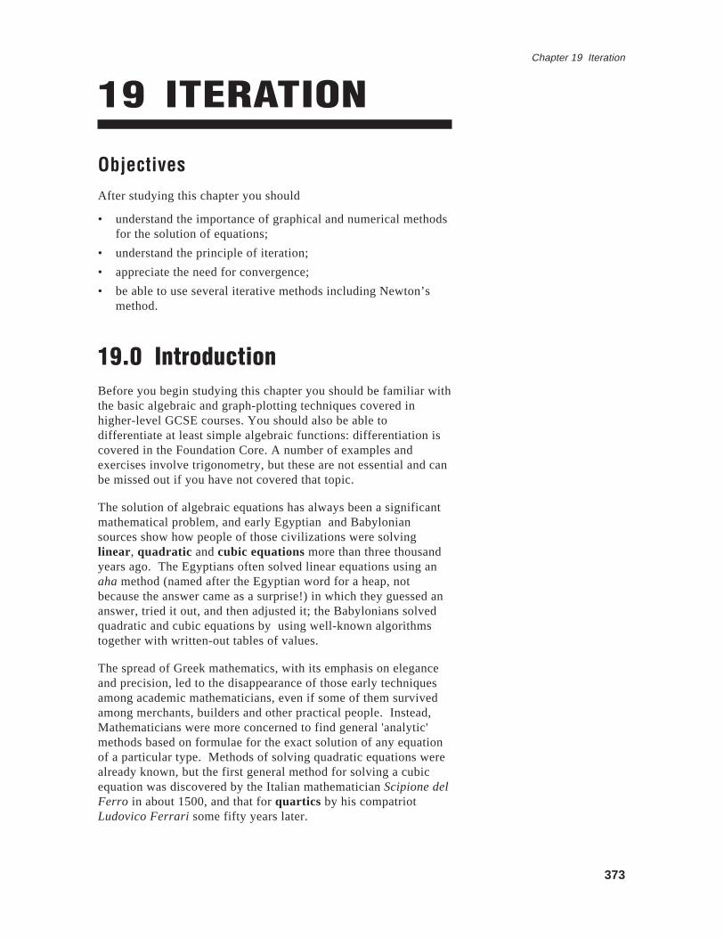
19.1 Crossing laddersIn a narrow passage between two walls there are two woodenladders, a green one 3 m long and a red one 2 m long; the groundis horizontal and the walls are vertical. Each ladder has its foot atthe bottom of one wall and its top resting against the other wall.The green ladder slopes up from left to right and the red ladderslopes up from right to left. The ladders cross 1 m above theground. How wide is the passage?
The first step in solving most problems of this kind is the creationof a mathematical model - not a model made of cardboard andglue, but a set of equations and other relations describing themathematically important features of the situation.
Stop and think what these important factors are.
The essential facts are summarised in the diagram opposite, whichshows the approximate positions and lengths of the ladders andthe position of their crossing point. It denotes by x metres thedistance to be found, and by u m, v m and w m respectively threeother lengths that may be important. The diagram says nothingabout the fact that the ladders are made of wood or that they aredifferently coloured, since these facts are irrelevant to theparticular problem to be solved.
From the diagram, various relationships can be deduced.
Using similar triangles,
w
1=
x
u
Again using similar triangles,
x − w
1=
x
v
u2
3
v
The ladder problem -find the length x
1
x
w

375
Chapter 19 Iteration
Adding these equations,
x
1=
x
u+
x
v
⇒
1
u+
1
v= 1
Now by Pythagoras’ theorem,
u2 + x2 = 4
⇒ u = 4 − x2
and similarly,
v2 + x2 = 9
⇒ v = 9− x2
giving
1
4 − x2+
1
9− x2= 1.
All that remains is to solve this equation, and the value obtainedfor x is the width of the passage in metres.
Consider how you might obtain a solution.
Several methods of solution are possible, but you should haverealised almost at once that this is not the sort of equation thatcan be solved by a simple algorithm (such as, “Take all the xterms to one side and all the numbers to the other”), nor is therea formula such as the one commonly used for quadraticequations. This equation cannot in fact be solved by any such'analytic' method. Instead we are going to resort to methodswhich will lead us to very accurate approximations to solutions.
There are two approaches which may work, one involvingnumerical substitution and the other based on graphs. If you canfind a positive numerical value for x which satisfies theequation, then clearly this is a solution. Random guessing islikely to take a long time, however, so any approach must bebased on some kind of systematic trial and improvement. Laterin this chapter several numerical methods are examined indetail. The alternative graphical approach is the subject of thenext section.
19.2 Graphical methodsYou should already be familiar with the idea of solving anequation by means of a graph: an example will remind you ofthe method.

376
Chapter 19 Iteration
ExampleSolve
x2 + 3x − 5 = 0.
Solution
The diagram shows the graph of
y = x2 + 3x − 5, plotted from atable of values in the usual way. It crosses the x-axis at thepoints
(− 4.2, 0 ) and (1.2, 0) approximately - the graph certainlycannot be read to an accuracy greater than one decimal place -so the solutions of the equation are
x ≈ − 4.2 and
x ≈ 1.2.
If you have the use of a graphic calculator or a computer withgraph-drawing facilities, you can get the same result with muchless effort. Draw the graph on the screen, and then use thecomputer mouse (or the <Trace> function on the calculator) tomove the cursor to each of the crossing points in turn.
The same method can be used more generally to solve equationsin higher powers of x. There are formulae (like the quadraticformula but much more complicated) for solving cubic andquartic equations, but the French mathematician Evariste Galoisproved just under 200 years ago that no such formula can everbe found for general equations in powers of x higher than thefourth. As a bonus, the graphical method works for equationsincluding sines, cosines, exponential and logarithmic functions,and so on. Look at some more examples.
ExampleSolve the equation
2x − 3 = 0.
Solution
The diagram shows the graph of
y = 2x − 3, plotted from a tableof values or drawn on a calculator or computer screen. Thegraph crosses the x-axis at (1.6, 0) approximately, and nowhereelse, so
x ≈ 1.6 is the only solution of the equation.
ExampleFind correct to one decimal place all the solutions of theequation
5cosx − x = 0 , where x is expressed in radians.
-2-4 2
4
-4
y
x
y = x2
+3x − 5
-6
4
y
8
x-2 2
y = 2x
− 3
-4

377
Chapter 19 Iteration
SolutionThe diagram shows the graph of
y = 5cosx − x . It crosses the x-axis three times, at (
−3.8, 0), (
−2.0, 0) and (1.3, 0), and so theequation has the three solutions,
x ≈ −3.8,
x ≈ −2.0, and
x ≈ 1.3.
Plotting two graphsThe equation in the last example could have been rewritten in theform
5cosx = x , so an alternative approach would have been toplot two graphs, the graph of
y = 5cosx and the graph of
y = x ,and to find their points of intersection. The advantage of thismethod is that both these are well-known functions whose graphsshould be familiar, making it quick and easy to draw them. Thediagram shows these two graphs, and it is evident that the valuesof x at the points of intersection correspond to those alreadyfound.
ExampleBy drawing two graphs, solve
x3 + 2x − 4 = 0.
SolutionThe equation can be written as
x3 = 4 − 2x , and the diagram showsthe graphs of
y = x3 and
y = 4 − 2x . They intersect only once, at(1.2, 1.6), so the only solution of this cubic equation is
x ≈ 1.2.
The equation could have been solved in other ways. It could have
been rearranged in the form
2x = 4 − x3 , or even as
x2 =4
x− 2,
and either of these would have given the same result. Often thereis no one right way to solve an equation graphically, but a wholecollection of ways, some of which may be easier than others.
A possible difficultyA particular difficulty arises when the graph is nearly flat at thepoint where it crosses the x-axis, or where two graphs are nearlyparallel at their point of intersection. The next example providesan illustration.
ExampleSolve the equation
3x = x2 + 2x .
-10
-5
5
10
y
-8 -4 x4 8
y = 5cosx − x
The graph crosses the x-axisthree times
-5
5y
x10-10
y = x
y = 5cosx
The two graphs intersect atthree points
-8
-4
y
4
8
-2 x2
y = 4− 2x
y = x3

378
Chapter 19 Iteration
SolutionThe first diagram opposite shows the graphs of
y = 3x and
y = x2 + 2x , and while it is clear that there is one root of theequation at
x ≈ −2.1, the other (or others?) could be almostanywhere between 1.0 and 2.0.
The second diagram showing the graph of
y = 3x − x2 − 2x is notmuch more helpful.
It is only in the third diagram with its exaggerated vertical scalethat the other two solutions can be identified as
x ≈ 1.0 (
x = 1 isactually an exact solution) and
x ≈ 1.6.
Exercise 19A
Use graphical methods to find approximate solutionsof the following equations, giving answers correct toone decimal place.
1.
x2 −1=1
x
19.3 Improving accuracyIn the previous section all the solutions were given correct toone decimal place, but this is not always good enough. Howmight you get a more accurate answer - to two or three decimalplaces, say?
Stop and think about how you could obtain a more accurateanswer.
You may have found a hint in the last example of Section 19.2 –with graphical methods, it is usually possible to get a moreaccurate answer by redrawing the graph on a larger scale. Thenext example illustrates this.
-4
-2
2
y4
-3 -2 -1 1 2 x
y = 3x − x2 − 2x
y = 3x
y = x2 +2x
-4
4
8
12
16
-3
y
-2 -1 1 2 x
-0.2
-0.15
-0.1
-0.05
y
0.05
-3 -2 -1 1 2 x
y = 3x − x2 − 2x
Function on a larger scale
2.
x3 − 6x2 +11x − 5 = 0
3.
x4 = 2x +1
4.
2x − 5x = 0
*5.
sinx = cos2x (answers between 0 and
2π only)

379
Chapter 19 Iteration
ExampleSolve
x3 + 2x2 − 5 = 0 , giving your answer correct to threedecimal places.
Solution
The first diagram shows the graph of
y = x3 + 2x2 − 5, plottedfor values of x between
−2 and 2. The equation clearly has onlyone root, which lies between 1 and 2, and a graphical estimatemight suggest
x ≈ 1.2 to one decimal place.
The second diagram shows the same graph, but this time plottedonly between
x = 1 and
x = 1.5 - notice that over this limiteddomain the graph is almost a straight line. On this larger scale itis possible to estimate the root more accurately, and to say that
x ≈ 1.24 to two decimal places.
The third diagram increases the scale yet again, and shows thegraph plotted over the domain
1.23≤ x ≤ 1.25. Now the
solution can be estimated even more accurately as
x ≈ 1.242 tothree decimal places. Clearly there is no limit in theory to theaccuracy that can be obtained by this method, but it is time-consuming.
Computers and calculatorsThe process can be carried out much more quickly with acomputer graph package or a graphic calculator. Most graph-drawing software packages allow the user to change the scaleswithout redrawing the whole graph, and by using this facility to'zoom in' on the root the solution can be read quite easily towhatever level of accuracy is required.
Activity 1 Graphic calculators
The <Factor> command on the Casio fx-7000G is not widelyused, but was designed for just this purpose. If you have such acalculator, try the following:
• <Range>
−10, 10, 5,
−10, 10, 5
• <Factor> 5 : <Graph>
Y = Xxy3+ 2X2 − 5 <EXE>
• <Trace> and use the
⇒and
⇐keys to move the flashing dotclose to the point where the graph crosses the x-axis, then<EXE> again.
• Repeat the last instruction as often as necessary - probably
1 1.5x
1
-1
The same graph for
1 ≤ x ≤ 1.5
y
......
x
0.1y
1.251.23
-0.1
......
The same again for
1.23≤ x ≤ 1.25
Graph of function for
−2 ≤ x ≤ 2
-6
-4
-2
2
4
y
-2 -1 1 x
y = x3
+ 2x2
−5

380
Chapter 19 Iteration
three or four times - until you are satisfied with the accuracyof the x-value given on the screen.
*AccuracyAlthough in theory there is no limit to the accuracy that can beobtained by a graphical method of this kind, it is difficult inpractice to get solutions correct to more than five or six decimalplaces. Unless you are fond of very cumbersome pencil-and-paper arithmetic you will almost certainly use a calculator towork out the values to plot, and most calculators operate to nomore than eight or ten significant figures at best. General-purpose computer packages have a similar limitation - sixsignificant figures is not uncommon - making it impossible toobtain any more accurate result unless you are prepared to adjustthe equation as well as the scales.
You should bear in mind too that many equations haveirrational solutions - that is, the 'true' solutions are numbers thatcannot be expressed exactly as fractions or decimals. Thusalthough it may be possible (in theory) to get as close to the truesolution as you might wish, you may never be able to find itsexact value. In real life this hardly matters - five or six decimalplaces is more than enough for any practical purpose - but amathematician would be careful to distinguish a good decimalapproximation from the 'exact' irrational solution.
Exercise 19B
Use a graphical method to solve each of thefollowing equations correct to the stated level ofaccuracy:
1.
x3 − 4x + 5 = 0 , to two decimal places
2.
x5 − x3 = 1, to two decimal places
19.4 Interval bisectionThe graphical method of solving equations, as you will haverealised, has two disadvantages. For one thing it tends to bequite time-consuming, though using a suitable calculator orcomputer can speed things up considerably. Secondly, however,it needs someone to read the graph, to estimate the position ofthe crossing point or move the cursor, and (if greater accuracy isrequired) to decide on the new range of values to be plotted.
3.
2x = x + 3 , to two decimal places (both solutions)
4.
2x2 +1=1
x, to three decimal places
*5.
x + ln x = 0 , to three decimal places

381
Chapter 19 Iteration
These disadvantages are overcome, at least in part, by some ofthe algebraic methods discussed in the rest of the chapter. Thechief benefit of such methods is that they can be expressedalgorithmically in terms of yes/no decisions and routineoperations, so eliminating the need for human intervention andmaking them suitable for programming into a computer orcalculator.
Activity 2 Guess a number
Take a few minutes to play this game with another student. Oneof you thinks of a whole number between 1 and 100, and theother has to guess this number by asking no more than tenquestions of a yes/no type. Play several rounds, taking it in turnsto be the guesser, and try to find the most efficient strategy.How many questions do you really need?
In fact seven questions and a final 'guess' will do, as long as thequestions are properly chosen. A skilful guesser might well haveasked questions like the following:
Is your number more than 50? Yes
Is it more than 75? No
Is it more than 62? Yes
Is it more than 69? Yes
Is it more than 72? No
Is it more than 70? Yes
Is it more than 71? Yes
The number is 72.
At each stage, the guesser is roughly halving the number ofpossibilities. Initially the number could be anywhere between 1and 100, but the first answer shows that it is actually between 51and 100. Then it is between 51 and 75, then between 63 and 75,then between 70 and 75, then between 70 and 72, then between71 and 72, and the final answer shows that it is 72.
If you played the game enough times you probably discoveredthis strategy (or something very similar) for yourself. If not,play two or three more rounds using this strategy, to be sure youunderstand how it works.
382
Chapter 19 Iteration
Locating a rootThe same principle, known as interval bisection because at eachstage the possible range of values is halved, can be applied to thesolution of equations. If you know that a particular equation hasa root between 2 and 3 (say), then you can ask whether the rootis greater than 2.5, and so halve the interval in which it is to befound. By doing this repeatedly, you can eventually say that theroot lies in an interval so small that you can give its value towhatever accuracy you want.
How do you find the first interval (i.e. between 2 and 3) ?
There are at least two practical methods of locating the root,either of which can be used alone but which are much better incombination. The first is to draw a quick rough graph; this doestake a little time, but it shows how many roots there arealtogether and helps you to avoid any of several possible traps.
The second method, which can be used on its own but which ismuch more reliable after you have sketched a graph, involveslooking for a change of sign. If you find, for example, that
f (2)
is negative and
f (3) positive, or vice versa, it follows that
provided f is a continuous function then
f (x) is zero somewhere
between
x = 2 and
x = 3.
The change-of-sign method is certainly more precise than thesketch graph in locating a root, but it does contain at least threepossible traps. Firstly, it may well locate one root but missanother: unless you are very persevering (or know where to look)you are unlikely to find a root between (say)
−11 and
−10.
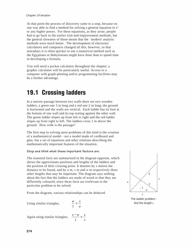
Secondly, the change-of-sign method will not work unless thegraph of
y = f (x) is continuous over the interval in question. Thediagram shows part of the graph of
y = tanx for values of x (in
radians) between 0 and 3. It is clear that
f (1) > 0and
f (2) < 0,
but equally clear that there is no root of the equation
f (x) = 0between 1 and 2.
Thirdly, the change-of-sign method will not show up repeatedroots (where the graph just touches the x-axis without crossingit), nor two roots close together. For example, the equation
6x2 − 29x + 35= 0 has solutions
x = 2 13 and
x = 2 12 , as you can
check by factorising, but
f (2) and
f (3) are both positive and sogive no indication that these roots exist.
In spite of these three problems, the change-of-sign method oflocating roots is very important, and useful too when properlyapplied in conjunction with a sketch. It forms the basis of theinterval bisection and linear interpolation methods discussed in
-4
-2
y
2
4
-1 x1 2
y = tanx
f (1) < 0 and f (2) < 2but there is no root between
1 and 2

383
Chapter 19 Iteration
this section and the next, and is commonly used at least at thestart of the more sophisticated methods of solution consideredlater in the chapter.
The method in practice
ExampleSolve
x4 − 2x3 −1= 0, correct to two decimal places.
SolutionThe diagram shows the graph of
y = x4 − 2x3 −1, and there areevidently two roots, one negative and close to
−1, and the otherpositive and close to 2.
f (−1) = 2 ,
f (0) = −1 and the change of sign shows that there is aroot between
−1 and 0.
f (2) = −1,
f (3) = 26 and the change of sign shows that thesecond root lies between 2 and 3.
Consider the positive root first.
f (2.5)≈ 6.8 so the change of sign is between 2 and 2.5.
f (2.2)≈ 1.1 so the change is between 2 and 2.2.
(This is not exactly the midpoint of the interval, but is nearenough and keeps the calculation fairly simple.)
f (2.1)≈ −0.1 so the change is between 2.1 and 2.2.
f (2.15)≈ 0.5 so the change is between 2.1 and 2.15.
f (2.12)≈ 0.1 so the change is between 2.1 and 2.12.
f (2.11)≈ 0.03 so the change is between 2.1 and 2.11.
f (2.105)≈ − 0.02 so the change is between 2.105 and 2.11.
This root is therefore 2.11 to two decimal places.
Similarly with the negative root,
f (− 0.5)≈ − 0.7 so the change is between
−1 and
− 0.5.
f (− 0.7)≈ − 0.1 so the change is between
−1 and
− 0.7.
f (− 0.85)≈ 0.8 so the change is between
− 0.85 and
− 0.7.
f − 0.78( ) ≈ 0.3 so the change is between
− 0.78 and
− 0.7.
-4
-2
2
4
y
-2 -1 1 2 x
y = x4
−2x2
−1
y = x4 − 2x
3 − 1

384
Chapter 19 Iteration
f (− 0.74)≈ 0.1 so the change is between
− 0.74 and
− 0.7.
f (− 0.72)≈ 0.02 so the change is between
− 0.72 and
− 0.7.
f (− 0.71)≈ −0.03 so the change is between
− 0.72 and
− 0.71.
f (− 0.715)≈ − 0.01 so the change is between
− 0.72 and
− 0.715.
So this root is
− 0.72 to two decimal places.
Exercise 19CUse a sketch graph followed by a change-of-signsearch to locate the roots of the equation
2x − 2x − 3 = 0 . Then use an interval bisection methodto find these solutions correct to two decimal places.
19.5 Rearrangement methodsInterval bisection is a fairly straightforward iterative method forthe solution of equations, but is not particularly efficient. Youhave seen in the examples and exercises that it may easily take sixor eight iterations to get a solution accurate to even two decimalplaces, and in a world where time is at a premium this is not goodenough. Other quicker methods must therefore be considered.
ExampleSolve the equation
x5 + 3x2 − 8 = 0.
SolutionLet
f (x) = x5 + 3x2 − 8 ; the graph of
y = f (x) shows clearly thatthere is only one root. Since
f (1) = − 4and
f (2) = 36, and since fis a continuous function, the solution lies between 1 and 2,probably close to 1.
Now the equation can be rearranged as
x5 = 8− 3x2 , and this in
turn can be written in the form
x= 8− 3x25. This equation can
then be used as the basis of an iteration formula; i.e. one where,given an approximation
x0 , a new approximation
x1 can be
calculated, and then a new approximation
x2 can be calculated,etc. In this case the formula is
xn+1 = 8− 3xn25 .
-15-10
-5
5
y
10
15
-2 -1 x1
y = x5
+ 3x2
− 8

385
Chapter 19 Iteration
Substituting the first approximation
x0 = 1 gives
x1 ≈ 1.4;substituting this result and then each of the others in turn gives
x2 ≈ 1.2,
x3 ≈ 1.3,
x4 ≈ 1.24,
x5 ≈ 1.28,
x6 ≈ 1.25,
x7 ≈ 1.27,
x8 ≈ 1.26 and
x9 ≈ 1.26 again. A quick check confirms that
f (1.255)< 0 and
f (1.265)> 0 , so that the solution is
x ≈ 1.26correct to two decimal places.
Although this has involved nine calculations (or iterations) andso is apparently no quicker than the previous methods, eachiteration involves no more than the substitution of the previousresult into a fairly simple formula. It is usually possible, in fact,to make the substitution using the value in the calculatordirectly, without the trouble of writing down each result and re-entering it: certainly a very simple program can be written for aprogrammable calculator or computer.
ExampleSolve
x2 + sinx = 1, with x in radians.
SolutionThe equation can be rearranged as
x2 = 1− sinx , and from asketch graph this has solutions at
x ≈ 0.6 and at
x ≈ −1.4. Therearrangement leads to an iteration formula
xn+1 = 1− sinxn
and substituting
x0 = 0.6 gives in turn
x1 ≈ 0.66,
x2 ≈ 0.622,
x3 ≈ 0.646,
x4 ≈ 0.631,
x5 ≈ 0.640, and
x6 ≈ 0.635. Once again
it is now easy to check that 0.635 and 0.645 give
x2 + sinxvalues respectively less than and greater than 1, so that thepositive solution is
x ≈ 0.64 to two decimal places.
Substituting
x0 = −1.4, on the other hand, gives
x1 ≈ 1.41 and
x2 ≈ 0.11 and gradually moves in to the same solution as before.This is because the iteration formula has taken the positivesquare root, and so naturally gives only positive results. Analternative iteration formula with a negative square root wouldbe equally valid:
xn+1 = − 1− sinxn
and with
x0 = −1.4 this gives
x1 ≈ x2 ≈ −1.41, which can bechecked as correct in the usual way.
-1
1
2
-4 -3
y
-2 -1 1 2 3 4 x
y = x2
y =1−sinx
-5

386
Chapter 19 Iteration
Exercise 19D
1. Show that the equation
x3 + 2x − 6 = 0 has justone solution, and locate it. Show that theequation can lead to the iteration formula
xn+1 = 6− 2xn3 ,
and use this formula to find the solution correctto two decimal places.
2. Write down the equation whose solution can befound by using the iteration formula
xn+1 = 1+1
xn2
,
and use the formula to find this solution correctto two decimal places.
19.6 ConvergenceExercise 19D should have started you thinking. Why is it, forexample, that in Question 3 one iteration formula would workonly for the smaller root and the other only for the greater? Whydo some formulae seem to work faster than others? Why dosome formulae not lead to a root at all, but give results thatswing wildly from side to side?
These are all questions concerned with the convergence of theiterative process, and while it is useful for you to have a generalunderstanding of the idea, you do not need to go deeply into thetheory. If you want to study convergence more deeply than thissection allows, look at an undergraduate textbook on numericalanalysis.
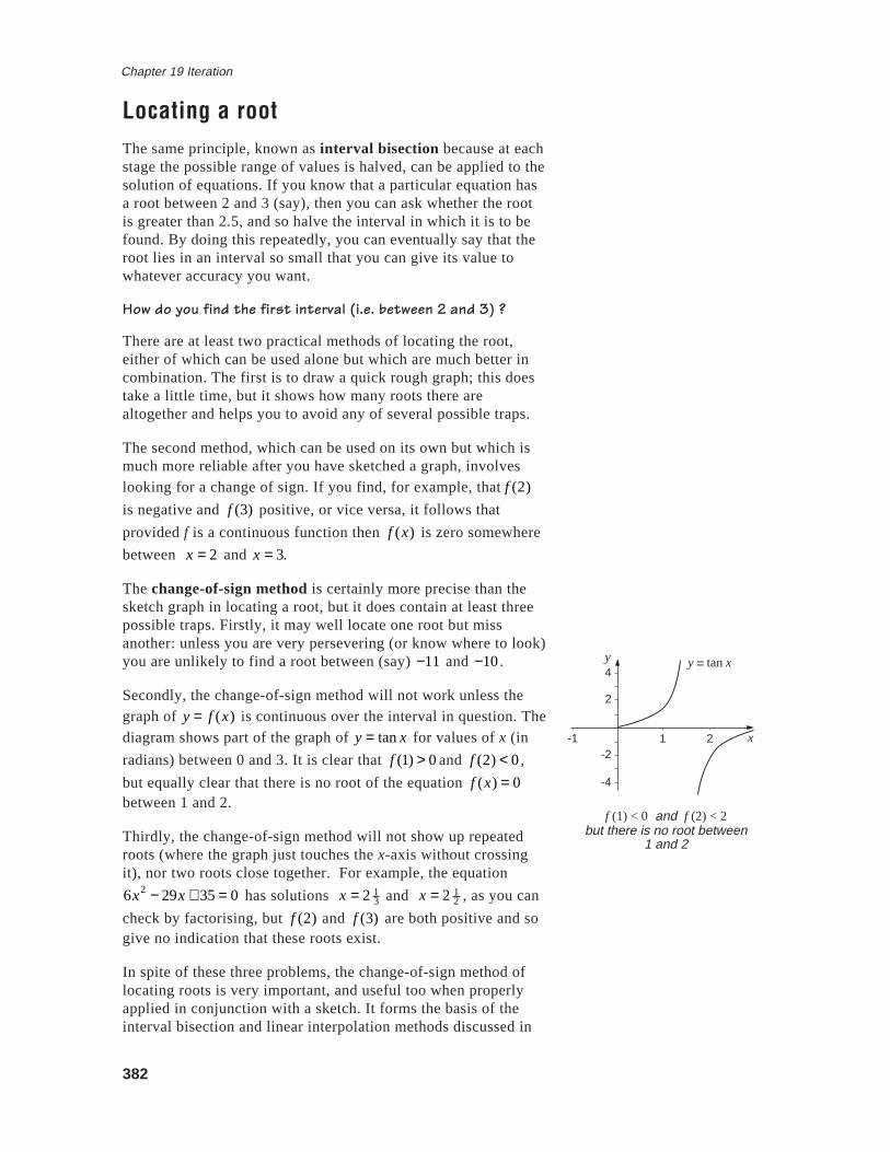
Consider the equation
x2 − 5x + 2 = 0 , to be solved using the
formula
xn+1 = 5xn − 2 . The diagram shows two graphs, those
of
y = x and
y = 5x − 2 respectively; their points ofintersection correspond to the solutions of the equation. The firstapproximation
x0 is substituted into the formula and gives a
value - call it
y0 - which then becomes
x1 : this process isillustrated by the arrows.
As the iteration is repeated, the arrows build into some sort ofpattern. In this particular case, they are moving (slowly) closerto the right-hand point of intersection, and so will eventuallylead to that solution.
If you try to apply the same method to find the left-hand point ofintersection, you will fail no matter how hard you try - thearrows will either converge onto the right-hand point or diverge
3. Show that the equation
x4 − 3x +1= 0 has twosolutions, and locate them approximately. Showthat the equation can lead to two iterationformulae
xn+1 = 3xn −14 and
xn+1 =xn
4 +1
3and show that each of these formulae leads to justone solution. Find each solution correct to twodecimal places.
4. Find a suitable iteration formula for the equation
x3 − x2 − 5 = 0 , and solve the equation correct totwo decimal places.
5. Use an iterative method to solve the equation
xx = 2 correct to three decimal places.
y
x
y = x
x0
x1
5
50
The principle of iteration
y = 5x − 2.......................
y0
387
Chapter 19 Iteration
altogether. On the other hand, the iteration formula
xn+1 =xn
2 + 2
5
(illustrated in a similar way in this diagram) converges quiteneatly onto the left-hand point of intersection and cannot bepersuaded to lead to the upper solution.
Test for convergenceIf you want to know whether or not a particular iterationformula will converge, it is often easiest in practice to apply theformula three or four times and look at the pattern of results. Ifthe results are getting gradually closer together they areprobably converging on a solution; if not, you are unlikely tofind the solution using this formula. There is a more formaltest, however, that you might want to use in a particular case.
Suppose that the iteration formula is
xn+1 = g(xn ) , and that thederivative of
g(x) is
g' (x) . Then it can be shown - the proof isnot attempted here - that a necessary and sufficient conditionfor the formula to converge on the true solution λ is that
−1< g' (λ ) < 1.
This condition is all very well, except that the value of
λ iswhat you are trying to find! In practice, therefore, it is usual tolook for an x-interval containing both the unknown λ and the
first approximation
x0 such that
g' (x) < 1 throughout the
interval. In the example above, if
g(x) = 5x − 2 then
g' (x) =5
2 5x − 2. This has absolute value less than 1 if
x > 1.65,
and so can converge on the upper solution (given a suitable firstapproximation) but not the lower. On the other hand, if
g(x) =x2 + 2
5 then
g' (x) =2x
5, which lies between
−1 and 1
only when
−2.5< x < 2.5; it thus converges only to the lowersolution.
Exercise 19EUse a graph to locate approximately the root or rootsof each of the equations opposite. Rearrange eachequation to give an iteration formula, and test eachformula to determine whether it will lead to any orall of the roots. Repeat with another rearrangementif necessary, until all the roots are obtainable. Findeach root correct to one decimal place.
An alternative iteration formula forthe lower root
y =x2 + 2
5
1.
x3 − 3x − 4 = 0
2.
x4 + 2x3 = 5.
3.
3x = 3x + 2 .
388
Chapter 19 Iteration
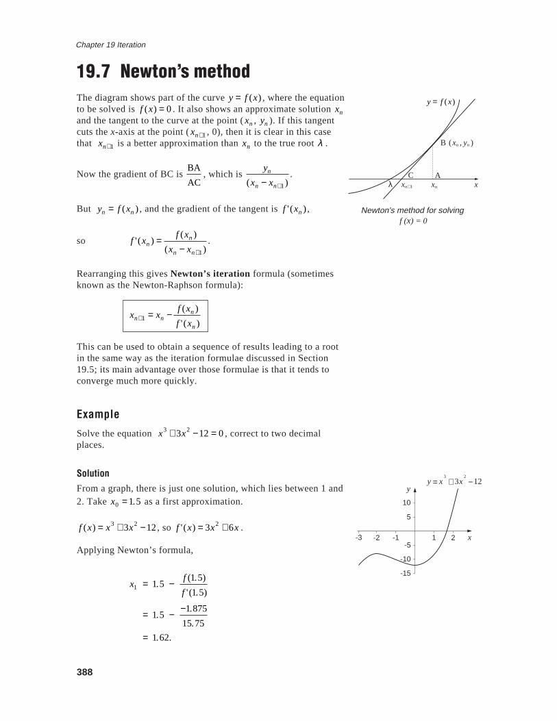
19.7 Newton’s methodThe diagram shows part of the curve
y = f (x) , where the equationto be solved is
f (x) = 0. It also shows an approximate solution
xn
and the tangent to the curve at the point (
xn ,
yn ). If this tangentcuts the x-axis at the point (
xn+1, 0), then it is clear in this casethat
xn+1 is a better approximation than
xn to the true root
λ .
Now the gradient of BC is
BA
AC, which is
yn
(xn − xn+1).
But
yn = f (xn ) , and the gradient of the tangent is
f ' (xn ) ,
so
f ' (xn ) =f (xn )
(xn − xn+1).
Rearranging this gives Newton’s iteration formula (sometimesknown as the Newton-Raphson formula):
xn+1 = xn −f (xn )
f ' (xn )
This can be used to obtain a sequence of results leading to a rootin the same way as the iteration formulae discussed in Section19.5; its main advantage over those formulae is that it tends toconverge much more quickly.
Example
Solve the equation
x3 + 3x2 −12 = 0 , correct to two decimalplaces.
SolutionFrom a graph, there is just one solution, which lies between 1 and2. Take
x0 = 1.5 as a first approximation.
f (x) = x3 + 3x2 −12, so
f ' (x) = 3x2 + 6x .
Applying Newton’s formula,
x1 = 1.5 −f (1.5)
f ' (1.5)
= 1.5 −−1.875
15.75
= 1.62.
Newton's method for solving f (x) = 0
λ
xn+1
xn
B
(xn , yn )
ACx
y = f (x)
-15
-10
-5
5
10
-3
y
-2 -1 1 2 x
y = x3
+ 3x2
−12
389
Chapter 19 Iteration
Applying the formula again,
x2 = 1.62 −f (1.62)
f ' (1.62)
= 1.62 −0.125
17.59
= 1.613.
And it is not difficult now, after just two iterations, to check that
f (1.605)< 0 and that
f (1.615)> 0 , so giving
x ≈ 1.61 correct totwo decimal places.
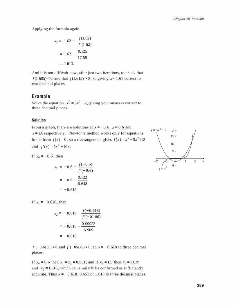
ExampleSolve the equation
x5 = 5x2 − 2, giving your answers correct tothree decimal places.
Solution
From a graph, there are solutions at
x ≈ − 0.6,
x ≈ 0.6 and
x ≈ 1.6respectively. Newton’s method works only for equations
in the form
f (x) = 0 , so a rearrangement gives
f (x) = x5 − 5x2 + 2
and
f ' (x) = 5x4 −10x .
If
x0 = − 0.6, then
x1 = − 0.6 −f (− 0.6)
f ' (− 0.6)
= − 0.6 −0.122
6.648
= − 0.618.
If
x1 = − 0.618, then
x2 = − 0.618−f (− 0.618)
f ' (− 0.186)
= − 0.618−0.00023
6.909
= − 0.618.
f ' (− 0.6185)< 0 and
f ' (− 06175)> 0, so
x ≈ − 0.618 to three decimalplaces.
If
x0 = 0.6 then
x1 = x2 = 0.651; and if
x0 = 1.6 then
x1 = 1.619
and
x2 = 1.618, which can similarly be confirmed as sufficiently
accurate. Thus
x ≈ − 0.618, 0.651 or 1.618 to three decimal places.
-5
5
10
15
-2
y
-1 1 2 x
y = 5x2 − 2
y = x5

390
Chapter 19 Iteration
Example
Solve
cosx = x3, where x is in radians, correct to three decimalplaces.
SolutionA sketch graph shows just one root, close to 0.9. Rearranging the
equation gives
f (x) = cosx − x3 and
f ' (x) = −sinx − 3x2 .
If
x0 = 0.9,
x1 = 0.9 −− 0.107
−3.213= 0.867
x2 = 0.867−− 0.0046
−3.017= 0.866
x3 = 0.866−− 0.0016
−3.0116= 0.865.
Since
f (0.8645)> 0 and
f (0.8655)< 0,
x ≈ 0.865 correct to threedecimal places.
Evaluation of Newton’s methodThere is no doubt that Newton’s method is a very useful one, andit does have certain advantages over the methods discussedearlier. It converges much faster than any of the previous methodsand also the same formula can be used for each of the roots.
The method is not perfect, however, and it does have a number ofdisadvantages. The first of these is that
f (x) has to bedifferentiated, and your ability to do this will depend on yourknowledge of calculus techniques. Then, the first approximationmust normally be fairly close to the root you are trying to find,making a reasonable graph almost essential. Finally, the methodcan become unreliable if the graph of
y = f (x) has a turning pointor inflexion close to the root - in such a case a different iterativemethod may prove more effective.
In general, however, you will find the most effective strategy forthe solution of difficult equations to be the following:
1. Draw a graph or graphs to locate the root(s) approximately.
2. Use a change of sign and a single linear interpolation to geta good first approximation.
3. Apply Newton’s method once or twice (or more).
4. Verify that your answer has the accuracy you require.
-5
-2
2
y
-3 1 x3-1
y = x3
y = cosx

391
Chapter 19 Iteration
Exercise 19F
1. Show that the equation
x3 − 2x2 + 4 = 0 has a rootclose to
x = −1. Use Newton’s method to findthis root correct to two decimal places.
2. Find correct to three decimal places the smallestpositive root of the equation
x4 − 3x3 + 5x2 −1= 0 .
3. Use Newton’s method to find both solutions ofthe equation
x = 3lnx to three decimal places.
19.8 The ladders againWith the techniques covered in this chapter it is possible tocomplete the solution of the ladder problem introduced inSection 19.1. The problem, you will recall, was as follows:
In a narrow passage between two walls there are two woodenladders, a green one 3 m long and a red one 2 m long. Eachladder has its foot at the bottom of one wall and its top restingagainst the other wall. The green ladder slopes up from left toright and the red ladder slopes up from right to left. The ladderscross 1 m above the ground. How wide is the passage?
This problem led to the equation
1
4 − x2+
1
9− x2= 1
which was left unsolved at that time.
Although it is possible to attempt a graphical or numericalsolution of the equation as it stands, it is probably better tosimplify it by getting rid of the fractions and the roots.Multiplying the whole equation by both square roots,
9− x2 + 4 − x2 = 4 − x2 9− x2 .
Squaring,
9− x2( ) + 2 9− x2 4 − x2 + 4 − x2( ) = 4 − x2( ) 9− x2( ) .
Collecting terms,
2 9− x2 4 − x2 = 4 − x2( ) 9− x2( ) − 9− x2( ) − 4 − x2( )= 23−11x2 + x4.
4. Find
103 using
x0 = 2 and two applications ofNewton’s method, and calculate the percentageerror from the 'true' value obtained from acalculator.
*5. Solve
xx = 5 correct to four decimal places.

392
Chapter 19 Iteration
Squaring again,
4 9− x2( ) 4 − x2( ) = 23−11x2 + x4( )2
144− 52x2 + 4x4 = 529− 506x2 +167x4 − 22x6 + x8
∴ x8 − 22x6 +163x4 − 454x2 + 385 = 0.
Now let
f (x) = x8 − 22x6 +163x4 − 454x2 + 385 and draw the
graph of
y = f (x) for
0 ≤ x ≤ 2, since any valid solution mustcertainly lie within these bounds.
The diagram shows the result, and it is clear that there are twosolutions, close to
x = 1.2 and
x = 1.9 respectively.
Now
f ' (x) = 8x7 −132x5 + 652x3 − 908x : this is the step whichperhaps justifies the algebra, because differentiating the originalequation would have been very messy.
Applying the Newton-Raphson formula with
x0 = 1.2,
x1 = 1.2− f (1.2)f ' (1.2)
= 1.2− 7.84−263
= 1.23 to two decimal places.
Similarly,
x2 = 1.23 again.
It is easy to check that
f (1.225)> 0 and
f 1.235( ) < 0,confirming that this solution is accurate to the nearestcentimetre.
Similarly, taking
x0 = 1.9,
x1 = 1.87 to two decimal places.
A second iteration gives 1.87 again and this solution of
f x( ) = 0can similarly be shown to have the necessary accuracy.However, a few moments of thought, possibly by sketching thepositions of the ladders, will show you that the passage certainlycannot be 1.87 m wide. Sometimes squaring the originalequation (as we have done in this case) leads to some phantomroots being introduced and so one ought to spend a little timechecking that the answer obtained does solve the originalproblems.
The other root of
x ≈ 1.23 does work and so the passagewaymust be approximately 123 cm wide.
*Activity 3 Iterative chaos
Use a computer or a programmable calculator to investigatesequences given by the iteration formula
xn+1 = kxn 1− xn( ) , with
x0 = 0.7, for different values of k between 1 and 4. The resultscould be quite chaotic!
-40
-30
-20
-10
0
y
0.5 1 1.5 2 x
y = f (x)
Graph of function for
0 ≤ x ≤ 2

393
Chapter 19 Iteration
19.9 Errors and error propagationErrors can occur in a variety of ways, for example:
(a) rounding errors – in which it is convenient to work with a
truncated decimal, such as 0.33 for
13 ;
(b) method errors – in which the method used to solve aproblem is only approximate, such as the Newton-Raphsonmethod for finding the roots of an equation;
(c) experimental errors – in which inaccuracies inmeasurements occur, such as measuring lengths to the nearestmillimetre;
(d) human errors – which we all make at times, but checkingand cross-checking helps to reduce their impact.
Of particular concern here are errors arising from (a) and (c).
Absolute and relative errorsThe absolute error is defined as
eabs = X − x = approx− exact( )where X is the approximate value of the exact value x.
Examples(a) If
x = 13 and X = 0.3, then
eabs = 0.3− 13 = 0.03333...
(b) If
x = 13 and X = 0.33, then
eabs = 0.33− 13 = 0.003333...
(c) If x is measured to the nearest centimetre as 12 cm, then
X = 12 cm, so the maximum and minimum possible valuesof x are 12.5 and 11.5 cm, respectively.
If
x = 12.5 cm, then
eabs = 12−12.5 = 0.5
and similarly, if
x = 11.5, then
eabs = 12−11.5 = 0.5,
so the maximum possible absolute error is 0.5.
The use of absolute errors as a measure of accuracy is fine if, forexample, you are making comparisons of approximations to theexact value, as in (a) and (b) above. They are not so useful if youare making comparisons of approximations to different exactvalues or are comparing the accuracy of measurements ofdifferent sizes.

394
Chapter 19 Iteration
To overcome this difficulty, we use the concept of relativeerror defined by
erel = eabs
x
Examples
(a) If
x = 13 and X = 0.3, then
erel = 0.0333...13
= 0.1.
(b) If
x = 5 13 and X = 5.3, then
erel = 0.03333...5 1
3
= 0.00625.
(c) Measuring x as 12 cm, to the nearest centimetre, implies
11.5≤ x ≤ 12.5, so
maximum
eabs = 0.5
giving maximum
erel = max eabs
min x= 0.5
11.5≈ 0.043.
(d) Measuring x as 1020 cm, to the nearest centimetre, implies
1019.5≤ x ≤ 1020.5, so
maximum
eabs = 0.5 (as in (c))
but maximum
erel = 0.51019.5
≈ 0.00049.
So the relative error is a better concept to use when makingcomparisons
(i) between errors in approximations to different exact values,
(ii) between the accuracy of measurements of different sizes.
In some cases, the exact value of x is unknown, so
x isapproximated by
X in the formula to give
estimated relative error = eabs
X
For example, if x is measured as 12 cm, to the nearestcentimetre, then
estimated relative error = 0.512
≈ 0.042.
Propagation of errorsWhen two numbers are multiplied together, the magnitude of therounding error may be larger than the rounding errors in the twonumbers. For example, if the two numbers, 4.2 and 1.1, are

395
Chapter 19 Iteration
given correct to one decimal place, then the product is
4.2×1.1= 4.62.
However, the first number could be between 4.15 and 4.25, andthe second between 1.05 and 1.15. So the maximum value ofthe product is
4.25×1.15= 4.8875
and the minimum value is
4.15×1.05= 4.3575.
So the error interval is now 4.3575 to 4.8875 – a range of 0.53,compared to the error range of 0.1 in each number.
ExampleFind the maximum possible value of the volume of a cylinderwhen the radius and height are measured, correct to thenearest mm, as
r = 4.2 cm, h = 8.6 cm.
SolutionThe volume is given by
V = π r 2h = π × 4.2( )2 × 8.6≈ 476.6 cm3
whilst the maximum possible value of V is given by
V = π× 4.25( )2 × 8.65≈ 490.8 cm3 .
ExampleFind the maximum possible value of x when evaluating theexpression
x = 2.7× 3.6( ) − 4.2
3.5+ 8.7 ≈ 0.4525( )
where each number is given correct to one decimal place. Alsofind an estimate for the percentage error.
SolutionThe maximum possible value of x is given by
maximum numeratorminimum denominator
= 2.75× 3.65( ) − 4.15
3.45+ 8.65≈ 0.4866

396
Chapter 19 Iteration
The percentage (%) error can be estimated as
0.4866− 0.4525( )0.4525
×100= 7.53%
which assumes that the true value of x is 0.4525.
Activity 4
Also find the minimum possible value for the expression.
What is the percentage error using the expression if the truevalue is either the maximum or minimum value of theexpression?
19.10 Miscellaneous Exercises1. Show that the equation
x3 − x − 2 = 0 has onlyone real root, and that this root lies between 1and 2. Use an iterative method to determine itsvalue accurate to three decimal places.
2. Determine graphically the number of solutionsof the equation
x2 − 4 =1
x,
and estimate their values.
3. Show that the equation
2x = 3x + 2 has twosolutions, and find each of them correct to twodecimal places.
4. Find correct to two decimal places all thesolutions of the equation
x4 + 2x3 −11x2 −12x + 21= 0 .
5. Find correct to four decimal places the smallestpositive root of the equation
7x3 −19x2 +14x − 3 = 0 .
6. Solve the equation
x ex = 1, correct to twodecimal places.
7. Without using any calculator functions otherthan +, − ,
× and
÷ , find
3 correct to sixdecimal places.
8. Find correct to two decimal places thecoordinates of the points at which the circle
x2 + y2 = 16 meets the rectangular hyperbola
x(y +1) = 9 .
9. Show that
xn+1 = 9xn−5( )13
is an iteration formula for thesolution of the equation
x x2 − 9( ) + 5 = 0
Show that this equation has a root between – 4and – 3, and use the given iteration formula
with
x0 = −3 to find this root correct to 2decimal places, showing that your answer hasthis accuracy. (AEB)
*10. In a circle whose radius is 10 cm, a segment ofarea 50 cm2 is cut off by a chord AB. Show thatAB subtends an angle θ radians at the centre ofthe circle, where
θ − sinθ = 1 . Solve thisequation and hence find the perimeter of thesegment in cm correct to two decimal places.
11. Show that the equation
x3 − x2 − 2 = 0 has a root
α which lies between 1 and 2.
(a) Using 1.5 as a first approximation for
α , usethe Newton-Raphson method once to obtain asecond approximation for
α , giving youranswer to 3 decimal places.
(b) Show that the equation
x3 − x2 − 2 = 0 can be
arranged in the form
x = f x( )( )3 where
f x( )is a quadratic function.
Use an iteration of the form
xn+1 = g xn( )based on this rearrangement and with
x1 = 1.5
to find
x2 and x3, giving your answers to3 decimal places. (AEB)