chapter 18 · chapter 18 nodes and antinodes what you have observed is a stationary wave on the...

196

The waves we have considered so far in Chapter 15, Chapter 16 and Chapter 17 have been progressive waves; they start from a source and travel outwards. A second important class of waves is stationary waves (standing waves). These can be observed as follows.

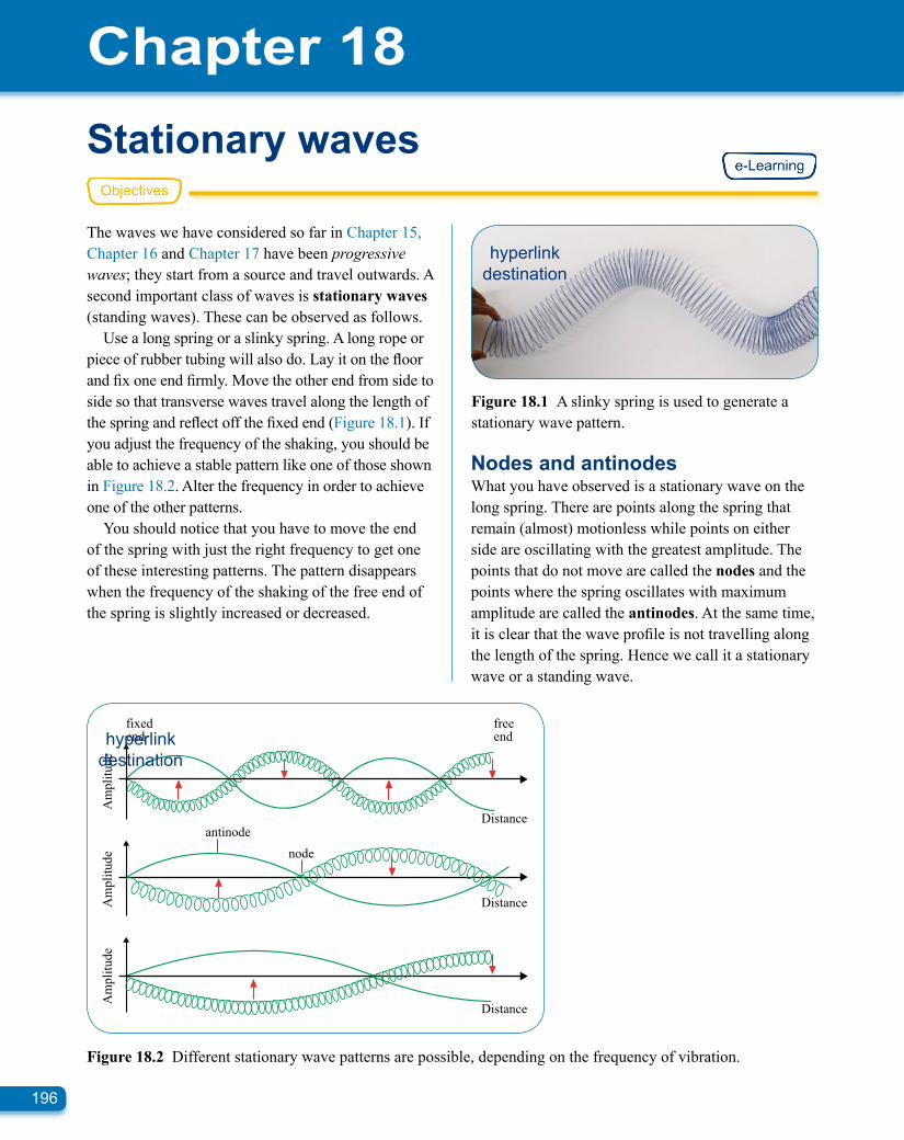
Use a long spring or a slinky spring. A long rope or piece of rubber tubing will also do. Lay it on the floor and fix one end firmly. Move the other end from side to side so that transverse waves travel along the length of the spring and reflect off the fixed end (Figure 18.1). If you adjust the frequency of the shaking, you should be able to achieve a stable pattern like one of those shown in Figure 18.2. Alter the frequency in order to achieve one of the other patterns.

You should notice that you have to move the end of the spring with just the right frequency to get one of these interesting patterns. The pattern disappears when the frequency of the shaking of the free end of the spring is slightly increased or decreased.

Stationary waves

Chapter 18

Nodes and antinodesWhat you have observed is a stationary wave on the long spring. There are points along the spring that remain (almost) motionless while points on either side are oscillating with the greatest amplitude. The points that do not move are called the nodes and the points where the spring oscillates with maximum amplitude are called the antinodes. At the same time, it is clear that the wave profile is not travelling along the length of the spring. Hence we call it a stationary wave or a standing wave.

fixed end

free end

Am

plitu

de

Am

plitu

de

Am

plitu

de

Distance

Distance

Distance

antinode node

Figure 18.2 Different stationary wave patterns are possible, depending on the frequency of vibration.

Figure 18.1 A slinky spring is used to generate a stationary wave pattern.

hyperlink destination


http://advancedsciences.cambridge.org/ocr/physics_1/18/EL/

J7007 CUP

0521787185c18_04.eps

resultant

wave moving to right

wave moving to left

wave moving to rightwave moving to leftresultant wave

Key

NN

A A A AA

N N N N

‘Snapshots’of the wavesover a timeof oneperiod, T.

T = period of wave

Distance

s

s

s

s

t = 0

t = T

Displacement λ

x

x

t =

profile at t = and

profile at t =

profile at t = 0 and T

x

x

t = T2

T4

t = 3T4

3T4

T4

T2

λ2

λ2

We normally represent a stationary wave by drawing the shape of the spring in its two extreme positions (Figure 18.3a). The spring appears as a series of loops, separated by nodes. In this diagram, point A is moving downwards. At the same time, point B in the next loop is moving upwards. The phase difference between points A and B is 180°. Hence the sections of spring in adjacent loops are always moving in antiphase; they are half a cycle out of phase with one another.

a

b

B

A

Distance

Am

plitu

de

Am

plitu

de

Distance

λ

Figure 18.3 The fixed ends of a long spring must be nodes in the stationary wave pattern.

Formation of stationary wavesImagine a string stretched between two fixed points, for example a guitar string. Pulling the middle of the string and then releasing it produces a stationary wave. There is a node at each of the fixed ends and an antinode in the middle. Releasing the string produces two progressive waves travelling in opposite directions. These are reflected at the fixed ends. The reflected waves combine to produce the stationary wave.

Figure 18.1 shows how a stationary wave can be set up using a long spring. A stationary wave is formed whenever two progressive waves of the same amplitude and wavelength, travelling in opposite directions, superimpose. Figure 18.4 uses a displacement s against distance x graph to illustrate the formation of a stationary wave along a long spring (or a stretched length of string).

• At time t = 0, the progressive waves travelling to the left and right are in phase. The waves combine constructively giving amplitude twice that of each wave.

• After a time equal to one quarter of a period (t = T4 ), each wave travels a distance of one quarter of a wavelength to the left or right. Consequently, the two waves are in antiphase (phase difference = 180°). The waves combine destructively giving zero displacement.

Figure 18.4 The blue-coloured wave is moving to the left and the red-coloured wave to the right. The principle of superposition of waves is used to determine the resultant displacement. The profile of the long spring is shown in green.

Chapter 18: Stationary waves

197




198

• After a time equal to one half of a period (t = T2 ), the two waves are back in phase again. They once again combine constructively.

• After a time equal to three quarters of a period (t = 3T

4 ), the waves are in antiphase again. They combine destructively with the resultant wave showing zero displacement.

• After a time equal to one whole period (t = T), the waves combine constructively. The profile of the slinky spring is as it was at t = 0.

This cycle repeats itself, with the long spring showing nodes and antinodes along its length. The separation between adjacent nodes or antinodes tells us about the progressive waves that produce the stationary wave.

A closer inspection of the graphs in Figure 18.4 shows that the separation between adjacent nodes or antinodes is related to the wavelength λ of the progressive wave. The important conclusions are:

separation between two adjacent nodes (or antinodes) =

λ2

separation between adjacent node and antinode = λ4

The wavelength λ of any progressive wave can be determined from the separation between neighbouring nodes or antinodes of the resulting standing wave pattern. (This is = λ

2 .) This can then be used to determine either the speed v of the progressive wave or its frequency f by using the wave equation:

v = f λ

It is worth noting that a stationary wave does not travel and therefore has no speed. It does not transfer energy between two points like a progressive wave. Table 18.1 shows some of the key features of a progressive wave and its stationary wave.

Progressive wave

Stationary wave

wavelength λ λ

frequency f f

speed v zero

Table 18.1 A summary of progressive and stationary waves.

SAQ1 A stationary (standing) wave is set up on a

vibrating spring. Adjacent nodes are separated by 25 cm. Determine:a the wavelength of the stationary

waveb the distance from a node to an

adjacent antinode.

Observing stationary waves

Stretched stringsA string is attached at one end to a vibration generator, driven by a signal generator (Figure 18.5). The other end hangs over a pulley and weights maintain the tension in the string. When the signal generator is switched on, the string vibrates with small amplitude. However, by adjusting the frequency, it is possible to produce stationary waves whose amplitude is much larger.

pulleyvibrationgenerator

weights

signalgenerator

Figure 18.5 Melde’s experiment for investigating stationary waves on a string.

The pulley end of the string is unable to vibrate; this is a node. Similarly, the end attached to the vibrator is only able to move a small amount, and this is also a node. As the frequency is increased, it is possible to observe one loop (one antinode), two loops, three loops and more. Figure 18.6 shows a vibrating string where the frequency of the vibrator has been set to produce two loops.




199

A flashing stroboscope is useful to reveal the motion of the string at these frequencies, which look blurred to the eye. The frequency of vibration is set so that there are two loops along the string; the frequency of the stroboscope is set so that it almost matches that of the vibrations. Now we can see the string moving ‘in slow motion’, and it is easy to see the opposite movements of the two adjacent loops.

This experiment is known as Melde’s experiment, and it can be extended to investigate the effect of changing the length of the string, the tension in the string and the thickness of the string.

SAQ2 Look at the stationary (standing) wave on the

string in Figure 18.6. The length of the vibrating section of the string is 60 cm.a Determine the wavelength of the stationary

wave and the separation of the two neighbouring antinodes.

The frequency of vibration is increased until a stationary wave with three antinodes appears on the string.b Sketch a stationary wave

pattern to illustrate the appearance of the string.

c What is the wavelength of this stationary wave?

MicrowavesStart by directing the microwave transmitter at a metal plate, which reflects the microwaves back towards the source (Figure 18.7). Move the probe

Figure 18.6 When a stationary wave is established, one half of the string moves upwards as the other half moves downwards. In this photograph, the string is moving too fast to observe the effect.

receiver around in the space between the transmitter and the reflector and you will observe positions of high and low intensity. This is because a stationary wave is set up between the transmitter and the sheet; the positions of high and low intensity are the antinodes and nodes respectively.

If the probe is moved along the direct line from the transmitter to the plate, the wavelength of the microwaves can be determined from the distance between the nodes. Knowing that microwaves travel at the speed of light c (3.0 × 108 m s–1), we can then determine their frequency f using the wave equation c = f λ.

reflectingsheet

probe

meter

microwave transmitter

Figure 18.7 A stationary wave is created when microwaves are reflected from the metal sheet.

SAQ3 a Draw a stationary wave pattern for the

microwave experiment above. Clearly show whether there is a node or an antinode at the reflecting sheet.

b The separation of two adjacent points of high intensity is found to be 14 mm. Calculate the wavelength and frequency of the microwaves.




200

Sound waves in air columnsA glass tube (open at both ends) is clamped so that one end dips into a cylinder of water; by adjusting its height in the clamp, you can change the length of the column of air in the tube (Figure 18.8). When you hold a vibrating tuning fork above the open end, the air column may be forced to vibrate, and the note of the

tuningfork

air

water

λ–4

Figure 18.8 A stationary wave is created in the air in the tube when the length of the air column is adjusted to the correct length.

tuning fork sounds much louder. This is an example of a phenomenon called resonance. The experiment described here is known as the resonance tube.

For resonance to occur, the length of the air column must be just right. The air at the bottom of the tube is unable to vibrate, so this point must be a node. The air at the open end of the tube can vibrate most freely, so this is an antinode. Hence the length of the air column must be one-quarter of a wavelength (Figure 18.9a). (Alternatively, the length of the air column could be set to equal three-quarters of a wavelength – see Figure 18.9b.)

SAQ4 Explain how two sets of identical but oppositely

travelling waves are established in the microwave and air column experiments described above.

Stationary waves and musical instrumentsThe production of different notes by musical instruments often depends on the creation of stationary waves (Figure 18.10). For a stringed instrument such as a guitar, the two ends of a string are fixed, so nodes must be established at these points. When the string is plucked half-way along its length, it vibrates with an antinode at its midpoint. This is known as the fundamental mode of vibration of the string. The fundamental frequency is the minimum frequency of a standing wave for a given system or arrangement.

antinode

node

antinode

node

a b

λ–4

3λ–4

Figure 18.9 Stationary wave patterns for air in a tube with one end closed.

Figure 18.10 When a guitar string is plucked, the vibrations of the strings continue for some time afterwards. Here you can clearly see a node close to the end of each string.






201

Similarly, the air column inside a wind instrument is caused to vibrate by blowing, and the note that is heard depends on a stationary wave being established. By changing the length of the air column, as in a trombone, the note can be changed. Alternatively, holes can be uncovered so that the air can vibrate more freely, giving a different pattern of nodes and antinodes.

In practice, the sounds that are produced are made up of several different stationary waves having different patterns of nodes and antinodes. For example, a guitar string may vibrate with two antinodes along its length. This gives a note having twice the frequency of the fundamental, and is described as a harmonic of the fundamental. The musician’s skill is in stimulating the string or air column to produce a desired mixture of frequencies.

J7007CUP

0521787185c18_11.eps

= Lλ

λ

L = length of string

fundamental = 2Lλ f0

2f0

= L 3f0

wavelength frequency

second harmonic

third harmonic

A

A A

AA A

N N

N NN

N NNN 23

Figure 18.11 Some of the possible stationary waves for a fixed string of length L. The frequency of the harmonics is a multiple of the fundamental frequency f0.

The frequency of a harmonic is always a multiple of the fundamental frequency. The diagrams show some of the modes of vibrations for a fixed length of string (Figure 18.11) and an air column in a tube of a given length that is closed at one end (Figure 18.12).

Determining the wavelength and speed of soundSince we know that adjacent nodes (or antinodes) of a stationary wave are separated by half a wavelength, we can use this fact to determine the wavelength λ of a progressive wave. If we also know the frequency f of the waves, we can find their speed v using the wave equation v = f λ.

J7007CUP

0521787185c18_12.eps

L = lengthof air

column

fundamental secondharmonic

thirdharmonic

= 4L

f0

=

3f0

wavelength

frequency

N

A

N

A

N

A

NANANA

4L3 =

5f0

4L5λ λ λ

Figure 18.12 Some of the possible stationary waves for an air column, closed at one end. The frequency of each harmonic is an odd multiple of the fundamental frequency f0.



Figure 18.13 Kundt’s dust tube can be used to determine the speed of sound.

One approach uses Kundt’s dust tube (Figure 18.13). A loudspeaker sends sound waves along the inside of a tube. The sound is reflected at the closed end. When a stationary wave is established, the dust (fine powder) at the antinodes vibrates violently. It tends to accumulate at the nodes, where the movement of the air is zero. Hence the positions of the nodes and antinodes can be clearly seen.

signal generator

loudspeaker

glass tube

closed end

dust piles up at nodes A

N A

N A

N A

An alternative method is shown in Figure 18.14; this is the same arrangement as used for microwaves. The loudspeaker produces sound waves, and these are reflected from the vertical board. The microphone detects the stationary sound wave in the space between the speaker and the board, and its output is displayed on the oscilloscope. It is simplest to turn off the time base of the oscilloscope, so that the spot no longer moves across the screen. The spot moves up and down the screen, and the height of the vertical trace gives a measure of the intensity of the sound.

By moving the microphone along the line between the speaker and the board, it is easy to detect nodes and antinodes. For maximum accuracy, we do not measure the separation of adjacent nodes; it is better to measure the distance across several nodes.

The resonance tube experiment (Figure 18.8) can also be used to determine the wavelength and speed of sound with a high degree of accuracy. However, to do this, it is necessary to take account of a systematic error in the experiment, as discussed in the ‘Eliminating errors’ section on page 203.

SAQ5 a For the arrangement shown in Figure 18.14,

suggest why it is easier to determine accurately the position of a node rather than an antinode.

b Explain why it is better to measure the distance across several nodes.

6 For sound waves of frequency 2500 Hz, it is found that two nodes are separated by 20 cm, with three antinodes between them.a Determine the wavelength of these sound

waves.b Use the wave equation v = f λ to determine

the speed of sound in air.

oscilloscope

loudspeaker

microphoneto signal generator(2 kHz)

reflectingboard

Figure 18.14 A stationary sound wave is established between the loudspeaker and the board.


202




203

The resonance tube experiment illustrates an interesting way in which one type of experimental error can be reduced or even eliminated.

Look at the representation of the stationary waves in the tubes shown in Figure 18.9. In each case, the antinode at the top of the tube is shown extending slightly beyond the open end of the tube. This is because experiment shows that the air slightly beyond the end of the tube vibrates as part of the stationary wave. This is shown more clearly in Figure 18.15.

J7007CUP

0521787185c18_15.eps

c

λ4

λ4

3

Figure 18.15 The antinode at the open end of a resonance tube is formed at a distance c beyond the open end of the tube.

for the shorter tube, λ4 = l1 + c

for the longer tube, 3λ4 = l2 + c

Subtracting the first equation from the second equation gives:

3λ4 –

λ4 = (l2 + c) – (l1 + c)

Simplifying gives:

λ2 = l2 – l1

and hence λ = 2(l2 – l1)

So, although we do not know the value of c, we can make two measurements (l1 and l2) and obtain an accurate value of λ. (You may be able to see from Figure 18.15 that the difference in lengths of the two tubes is indeed equal to half a wavelength.)

The end-correction c is an example of a systematic error. When we measure the length l of the tube, we are measuring a length which is consistently less than the quantity we really need to know (l + c). However, by understanding how the systematic error affects the results, we have been able to remove it from our measurements.

Other examples of systematic errors in physics include:

• meters and other instruments which have been incorrectly zeroed (so that they give a reading when the correct value is zero)

• meters and other instruments which have been incorrectly calibrated (so that, for example, all readings are consistently reduced by a factor of, say, 1.0%).

Eliminating errors

The antinode is at a distance c beyond the end of the tube, where c is called the end-correction. Unfortunately, we do not know the value of c. It cannot be measured directly. However, we can write:

SAQ7 In a resonance tube experiment, resonance is

obtained for sound waves of frequency 630 Hz when the length of the air column is 12.6 cm and again when it is 38.8 cm. Determine:

a the wavelength of the sound waves causing resonance

b the end-correction for this tubec the speed of sound in air.



204

Summary

• Stationary waves are formed when two identical waves travelling in opposite directions meet and superimpose. This usually happens when one wave is a reflection of the other.

• A stationary wave has a characteristic pattern of nodes and antinodes.

• A node is a point where the amplitude is always zero.

• An antinode is a point of maximum amplitude.

• Adjacent nodes (or antinodes) are separated by a distance equal to half a wavelength.

• We can use the wave equation v = f λ to determine the speed v or the frequency f of a progressive wave. The wavelength λ is found using the nodes or antinodes of the stationary wave pattern.

Questions1 The diagram shows a stretched wire held

horizontally between supports 0.50 m apart. When the wire is plucked at its centre, a

standing wave is formed and the wire vibrates in its fundamental mode (lowest frequency).

a Explain how the standing wave is formed. [2] b Draw the fundamental mode of vibration of the wire. Label the position of any

nodes with the letter N and any antinodes with the letter A. [2] c What is the wavelength of this standing wave? [1]OCR Physics AS (2823) January 2006 [Total 5]

2 The diagram shows an arrangement where microwaves leave a transmitter T and move in a direction TP which is perpendicular to a metal plate P.

a When a microwave detector D is slowly moved from T towards P the pattern of the signal strength received by D is high, low, high, low … etc.

Explain:

• why these maxima and minima of intensity occur

• how you would measure the wavelength of the microwaves

• how you would determine their frequency. [6] b Describe how you could test whether the microwaves leaving the transmitter are

plane polarised. [2]OCR Physics AS (2823) June 2004 [Total 8]

Answer

continued

D

T Ptransmitter

0.50 m


205

3 a In standing waves, there are nodes and antinodes. Explain what is meant by: i a node [1] ii an antinode. [1]

b The diagram shows a long glass tube within which standing waves can be set up. A vibrating tuning fork is placed above the

glass tube and the length of the air column is adjusted, by raising or lowering the tube in the water, until a sound is heard.

0.50m

tuning fork

0.32 m

water

air columnlong glass tube

A B

State how you would set up a standing wave on the string. [1] b The standing wave vibrates in its fundamental mode, i.e. the lowest frequency at

which a standing wave can be formed. Draw this standing wave. [1] c Figure 2 shows the appearance of another standing wave formed on the same string.

Figure 1

A B

Figure 2

The distance between A and B is 1.8 m. Use Figure 2 to calculate i the distance between neighbouring nodes [1] ii the wavelength of the standing wave. [1]

OCR Physics AS (2823) June 2003 [Total 4]

i The standing wave formed in the air column is the fundamental (the lowest frequency). Make a copy of the diagram and show on it the position of a node – label as N, and an antinode – label as A. [2]

ii When the fundamental wave is heard, the length of the air column is 0.32 m. Determine the wavelength of the standing wave formed. [1]

iii The speed of sound in air is 330 m s−1. Calculate the frequency of the tuning fork. [3]

OCR Physics AS (2823) June 2005 [Total 8]

4 a Figure 1 shows a string stretched between two points A and B.



chapter 18 · chapter 18 nodes and antinodes what you have observed is a stationary wave on the...

Documents