chapter 17 nuclear reactions - university of michiganners311/courselibrary/bookchapter17.pdf ·...

Chapter 17

Nuclear Reactions

Note to students and other readers: This Chapter is intended to supplement Chapter 11 of

Krane’s excellent book, ”Introductory Nuclear Physics”. Kindly read the relevant sections in

Krane’s book first. This reading is supplementary to that, and the subsection ordering will

mirror that of Krane’s, at least until further notice.

17.1 Types of Reactions and Conservation Laws

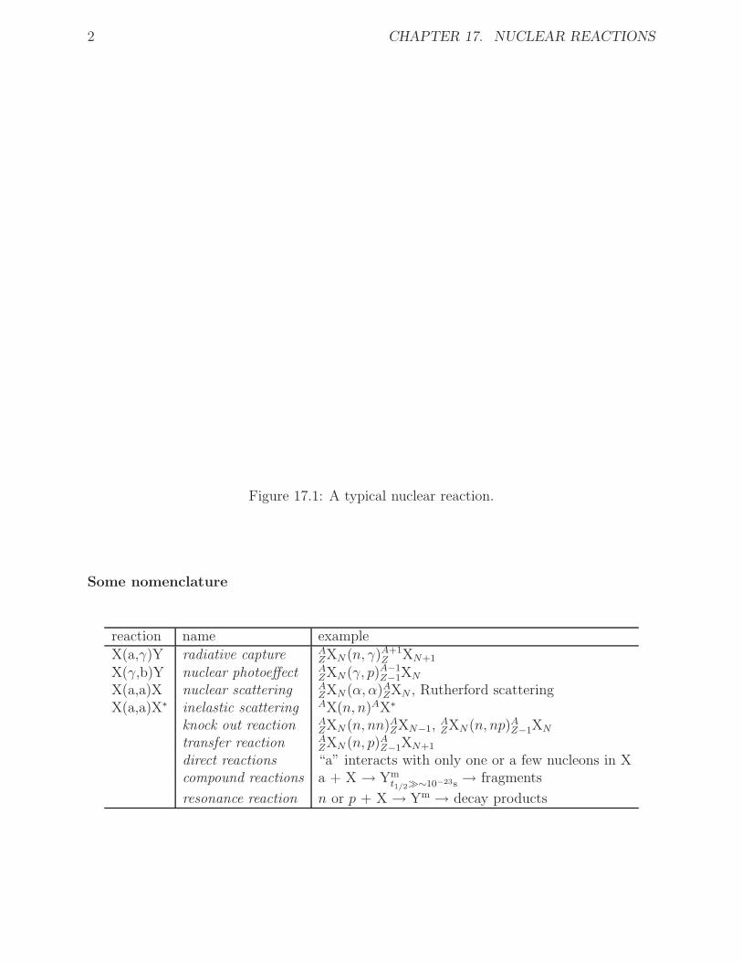
A typical nuclear reaction is depicted in Figure 17.1. The following two ways of describingthat reaction are equivalent:

a + X → Y + b ,

or

X(a, b)Y .

From now on, we shall usually use the latter because it is more compact (and easier to type!).

The above reaction is the kind we shall focus on because they represent most of the importantreactions in Nuclear Physics and Engineering and the Radiological Sciences. There are onlytwo bodies in the final state: a and Y. The particle labelled “a” is the projectile. Wewill generally restrict ourselves to considering light projectiles, with A ≤ 4, and projectileenergies, Ta . 10 MeV. The particle labelled “X” is to be thought of as the “target”. Theparticle labelled “b” is generally the lighter reaction product, and is often the particle thatis observed by the measurement apparatus. The remaining reaction product, is “Y”. Theis generally the heavier of the two reaction products, and is usually unobserved, as it stayswithin the target “foil”.

1

2 CHAPTER 17. NUCLEAR REACTIONS

Figure 17.1: A typical nuclear reaction.

Some nomenclature

reaction name example

X(a,γ)Y radiative capture AZXN (n, γ)A+1

Z XN+1

X(γ,b)Y nuclear photoeffect AZXN (γ, p)A−1

Z−1XN

X(a,a)X nuclear scattering AZXN (α, α)A

ZXN , Rutherford scatteringX(a,a)X∗ inelastic scattering AX(n, n)AX∗

knock out reaction AZXN (n, nn)A

ZXN−1,AZXN (n, np)A

Z−1XN

transfer reaction AZXN (n, p)A

Z−1XN+1

direct reactions “a” interacts with only one or a few nucleons in Xcompound reactions a + X → Ym

t1/2≫∼10−23s → fragments

resonance reaction n or p + X → Ym → decay products

17.1. TYPES OF REACTIONS AND CONSERVATION LAWS 3

17.1.1 Observables

Returning back to an X(a,b)Y reaction, the most comprehensive experiment one can performis to determine the b-particle type, and map out its angular distribution pattern, a so-called4π experiment. At each different angle, we also measure Tb, because that can change withdirection as well. Refer to Figure 17.2.

Figure 17.2: A typical set-up for a 4π experiment.

By knowing the intensity of the beam, we can thus compute the differential cross section,differential in Tb, θb, and φb, presented here in the 3 different forms that one encounters inthe literature.

dσ(Tb, θb, φb)

dΩbdTb

=dσ

dΩbdTb

= σ(Tb, θb, φb) , (17.1)

where dΩb is the differential solid angle associated with the direction of the b-particle,namely:


dΩb = sin θbdθbdφb .

The third form is favored by some authors (not me) because of its brevity. However, its useis common, and I wanted to familiarize you with it.

From this differential cross section, alternative, integrated forms my be found:

the cross section differential in angles only,

σ(θb, φb) =dσ

dΩb=

dσ(θb, φb)

dΩb=

∫

dTb

(

dσ(Tb, θb, φb)

dΩbdTb

)

, (17.2)

the cross section differential in energy only,

σ(Tb) =dσ

dTb=

dσ(Tb)

dTb=

∫

dΩb

(

dσ(Tb, θb, φb)

dΩbdTb

)

, (17.3)

and the total cross section,

σ =

∫

dTb

∫

dΩb

(

dσ(Tb, θb, φb)

dΩbdTb

)

. (17.4)

If one normalize (17.1) as follows:

p(Tb, θb, φb) =1

σ

dσ(Tb, θb, φb)

dΩbdTb

, (17.5)

p(Tb, θb, φb) is a “joint” probability distribution, properly normalized, over the variables, Tb,θb, and φb. From this probability distribution, we can determine quantities like, Tb, theaverage energy, or 1 − cos θb, the so-called scattering power.

17.1.2 Conservation laws

The conservation laws are essential tools in scattering analysis. Conservation of energy andlinear momentum allow us to deduce the properties of X and Y. Conservation of neutronand proton number also helps us deduce the properties of X and Y. Conservation of angularmomentum and parity, allow us to deduce spins and parities.

17.2. ENERGETICS OF NUCLEAR REACTIONS 5

17.2 Energetics of Nuclear Reactions

General Considerations in a Relativistic Formalism

For the X(a,b)Y reaction, conservation of Total Energy means:

mac2 +m

Xc2 + Ta + TX = m

bc2 +m

Yc2 + Tb + TY , (17.6)

or,

Q+ Ta + TX = Tb + TY , (17.7)

where,

Q ≡ (ma+m

X− [m

b+m

Y])c2 . (17.8)

Q is the reaction Q-value. When Q > 0, the reaction is exothermic (or exoergic). Energyis released by the transformation. When Q < 0, the reaction is endothermic (or endoergic).Energy is required, by the kinetic energies of the initial reactants, to make the transformation“go”.

Recall that (17.7) is a relativistic expression. Therefore, we should use relativistic expressionsfor the kinetic energies. Doing so,

Trel = mc2(γ − 1) . (17.9)

Since the maximum energy projectile we deal with is about 10 MeV, we have the situationwhere T ≪ mc2. Thus we can find a relationship that relates Trel, to its non-relativisticcounterpart, TNR:

Trel = TNR[1 +3

4β2 + O(β4)] . (17.10)

In the worst possible case (T = 10 MeV, mi = mp, the relativistic correction amounts to:

3

4β2 ∼= 3T

2mpc2∼= 0.015 . (17.11)

Therefore, in the worst possible Q = 0 case, there is a 1.5% correction, and up to double thatin the large Q case. This can be an important correction, depending on the accuracy of themeasurement. It represents a systematic error that may be swamped by other experimental


errors. However, from now on we shall ignore it, but keep in mind that large T and/or largeQ analyses, with small masses, may be problematic, unless we adopt a relativistic correction.

Photons are always relativistic. So, if they are involved, we use Tγ = Eγ, and Tγ/c for itsmomentum.

Laboratory frame, non-relativistic analysis

In the laboratory frame, in a non-relativistic analysis, we make the following approximations:

1) Ta < 10 MeV kinetic energy of the projectile2) ~pa = paz projectile’s direction is along the positive z-axis3) TX = 0 target is at rest4) 1 ≤ m

a, m

b≤ 4u small mass projectile, observed particle

5) mX, m

Y≥ 4u large mass target, unobserved particles

6) γi = 1 no relativistic corrections

With these approximations, Conservation of Energy and Conservation of Linear Momentumcan be expressed in the following equations:

Q+ Ta = Tb + TY , (17.12)

~pa

= ~pb+ ~p

Y. (17.13)

Since the Y-particle is unobserved, we choose to eliminate it from the (17.12) and (17.13),with the result:

Tb(mY+m

b) − 2

√

mam

bTa cos θb

√

Tb − [mY(Q+ Ta) −m

aTa] = 0 . (17.14)

This is a quadratic equation in√Tb, in terms of the (presumably) known quantities, Ta, Q,

and the masses. Solving the quadratic equation yields:

Tb =

√

mam

bTa cos θb ±

√

mam

bTa cos2 θb + (m

Y+m

b)[m

YQ+ (m

Y−m

a)Ta]

(mY

+mb)

. (17.15)

Thus, we see through (17.14), that 2-body reactions involve a direct correlation of the scat-tering angle, θb and the b-particle’s energy, Tb. Consequently, if one measures, Tb, and cos θbis also determined. The relationship between the two differential cross sections is:

dσ

dΩb=

dσ

dφbdTb

(

dTb

d(cos θb)

)

, (17.16)


or

dσ

dφbdTb=

dσ

dΩb

(

d(cos θb)

dTb

)

. (17.17)

The derivatives inside the large parentheses in (17.16) and (17.17) may be worked out from(17.14) and (17.15).

(17.15) may be complicated, but is is also very rich in physical content. Several interestingfeatures should be noted:

1. If Q > 0, then

√

mam

bTa cos θb <

√

mam

bTa cos2 θb + (m

Y+m

b)[m

YQ+ (m

Y−m

a)Ta] ,

and, therefore, we must always choose the positive sign in (17.15).

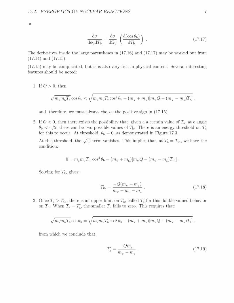
2. If Q < 0, then there exists the possibility that, given a a certain value of Ta, at e angleθb < π/2, there can be two possible values of Tb. There is an energy threshold on Ta

for this to occur. At threshold, θb = 0, as demonstrated in Figure 17.3.

At this threshold, the√

() term vanishes. This implies that, at Ta = Tth, we have thecondition:

0 = mam

bTth cos2 θb + (m

Y+m

b)[m

YQ+ (m

Y−m

a)Tth] .

Solving for Tth gives:

Tth =−Q(m

Y+m

b)

mY

+mb−m

a

. (17.18)

3. Once Ta > Tth, there is an upper limit on Ta, called T ′

a for this double-valued behavioron Tb. When Ta = T ′

a, the smaller Tb falls to zero. This requires that:

√

mam

bTa cos θb =

√

mam

bTa cos2 θb + (m

Y+m

b)[m

YQ+ (m

Y−m

a)Ta] ,

from which we conclude that:

T ′

a =−Qm

Y

mY−m

a

. (17.19)


Figure 17.3: Laboratory and center of momentum pictures of the X(a,b)Y interaction process.

4. For double-valued behavior on Tb, combining the results of (17.18) (17.19), we see thatTa must fall in the range:

mY

+mb

mY

+mb−m

a

≤ Ta

|Q| ≤m

Y

mY−m

a

. (17.20)

5. If Tth < Ta < T ′

a, there are also scattering angles for which double-valued behavior cannot exist. This happens when the argument of the

√

() falls to zero. This defines amaximum scattering angle for double-valued observation. From (17.15), we see thatthis maximum angle is given by:

cos2 θmaxb =

mY

+mm

mam

bTa

[−mYQ− (m

Y−m

a)Ta] (17.21)

These concepts are illustrated in Krane’s Figures 11.2(a) and 11.2(b) on pages 382–384,as well (eventually) in Figure 17.4.f


Figure 17.4: Demonstration of the double-valued nature of Tb.

Determining Q from scattering experiments

Up to now, we have assumed that Q was known. In some cases it is not, but, we candetermine it from a scattering experiment. Reorganizing (17.14) as follows,

Q = Tb

(

1 +m

b

mY

)

− Ta

(

1 +m

a

mY

)

− 2 cos θb

(

mam

b

m2Y

TaTb

)1/2

, (17.22)

appears that we have isolated Q. However, recalling the definition of Q,

Q ≡ (ma+m

X− [m

b+m

Y])c2 , (17.23)

our lack of knowledge of Q is tantamount to not knowing, at least with sufficient accuracy,one (or more) of the masses. For this type of experiment, it is usually the case, that m

Yis

the unknown factor. “X” is usually in the ground state, and hence, well characterized. “a”


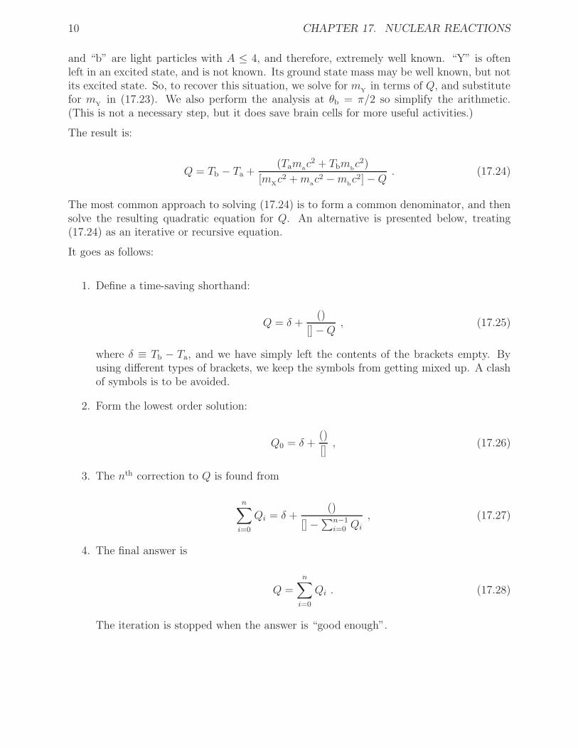
and “b” are light particles with A ≤ 4, and therefore, extremely well known. “Y” is oftenleft in an excited state, and is not known. Its ground state mass may be well known, but notits excited state. So, to recover this situation, we solve for m

Yin terms of Q, and substitute

for mY

in (17.23). We also perform the analysis at θb = π/2 so simplify the arithmetic.(This is not a necessary step, but it does save brain cells for more useful activities.)

The result is:

Q = Tb − Ta +(Tama

c2 + Tbmbc2)

[mXc2 +m

ac2 −m

bc2] −Q

. (17.24)

The most common approach to solving (17.24) is to form a common denominator, and thensolve the resulting quadratic equation for Q. An alternative is presented below, treating(17.24) as an iterative or recursive equation.

It goes as follows:

1. Define a time-saving shorthand:

Q = δ +()

[] −Q, (17.25)

where δ ≡ Tb − Ta, and we have simply left the contents of the brackets empty. Byusing different types of brackets, we keep the symbols from getting mixed up. A clashof symbols is to be avoided.

2. Form the lowest order solution:

Q0 = δ +()

[], (17.26)

3. The nth correction to Q is found from

n∑

i=0

Qi = δ +()

[] −∑n−1

i=0 Qi

, (17.27)

4. The final answer is

Q =

n∑

i=0

Qi . (17.28)

The iteration is stopped when the answer is “good enough”.


Illustration:

Q0 = δ +()

[]

Q0 +Q1 = δ +()

[] −Q0

Q0 +Q1 = δ +()

[]

(

1

1 −Q0/[]

)

Q0 +Q1 ≡ δ +()

[](1 +Q0/[])

Q0 +Q1 = Q0 +Q0()/[]2

Q1 = Q0()/[]2 (17.29)

Thus, the fractional correction is:

Q1

Q0=

(Tamac2 + Tbmb

c2)

[mXc2 +m

ac2 −m

bc2]2

. (17.30)

In the worst possible case, mX

= ma

= mb

∼= 4u, and Ta = Tb∼= 10 MeV, giving Q1/Q0

∼=5 × 10−3. Since Q-values are known typically to ≈ 1 × 10−4, this can be an importantcorrection, especially for small-A target nuclei.


17.3 Isospin

We know that the strong force does not distinguish between protons and neutrons (mostly).Therefore, one can consider this to be another kind ”of symmetry”, and symmetries havequantum numbers associated with them. Consider neutrons and protons to be two states ofa more general particle, called the nucleon, a name we have used throughout our discussions.However, now associate a new quantum number called “isospin”, with the symbol T3, andthe following numerical assignments.

particle T3

p +12

n −12

AZXN

12(Z −N)

Table 17.1: Isospin assignments

The assignment of the plus sign to the proton is completely arbitrary, but now part ofconvention.

Historically, isospin has been called isotopic spin, where a given Z, T3 combination identifies aspecific isotope associated with Z, or isobaric spin, where a given A, T3 combination identifiesa specific isobar associated with A. Today, “isospin” appears to be the preferred name.

As long as the strong force does not distinguish between isobars associated with a given A,we expect to see some similarity in the excitation levels associated with nuclei with the sameA. There is evidence for this, as seen in Figure 11.5 in Krane.

Isospins combine just as regular spins do. This is seen in the following example:

The dinucleon

Let us now consider the possible ways of combining two nucleons. We form the compositewavefunctions for two nucleons, one with spatial wavefunction ψ(~x1) and one with spatialwavefunction ψ(~x2). We label these as nucleon “1” and “2”. We also in include there isospinas either up. ↑, or down, ↓. Finally, since they are intrinsic spin-1

2particles, they must obey

the Pauli Exclusion Principle, and form composite wavefunctions that are antisymmetricunder the exchange of quantum numbers. Doing so, results in:

Note that the parity is associated with the space part of the wavefunction only. Also note,that the difference between the observed deuteron and its odd parity counterpart (unob-served) is how the antisymmetry is achieved. In the unobserved case, it is the spatial partthat is antisymmetrized, while the observed deuteron has a positive parity spatial wavefunc-tion and an antisymmetrized isopin wavefunction. In order to make full use of the attractivestrong force, the nucleons must come into close proximity. All of the members of the isobaric

17.4. REACTION CROSS SECTIONS 13

T T3 composite wavefunction π

1 1 2−1/2[ψ1(~x1)ψ2(~x2) − ψ1(~x2)ψ2(~x1)](↑1↑2) -1 diproton1 0 2−1[ψ1(~x1)ψ2(~x2) − ψ1(~x2)ψ2(~x1)](↑1↓2 + ↓1↑2) -1 odd parity deuteron?1 -1 2−1/2[ψ1(~x1)ψ2(~x2) − ψ1(~x2)ψ2(~x1)](↓1↓2) -1 dineutron0 0 2−1[ψ1(~x1)ψ2(~x2) + ψ1(~x2)ψ2(~x1)](↑1↓2 − ↓1↑2) +1 Deuteron

Table 17.2: The dinucleon quantum states

triplet have antisymmetric spatial wavefunctions. That is why none are bound.

17.4 Reaction Cross Sections

Covered elsewhere, and partly in 311.

17.5 Experimental Techniques

Not covered in 312.

17.6 Coulomb Scattering

Covered in 311.

17.7 Nuclear Scattering

Covered in Chapter 10.

17.8 Scattering and Reaction Cross Sections

Consider a z-direction plane wave incident on a nucleus, as depicted in Figure 17.5.

The wavefunction for the incident plane wave:

ψinc = Aeikz . (17.31)


Figure 17.5: Scattering of a plane wave from a nucleus.

We have seen elsewhere, that (17.31) is a solution to the Schrodinger equation in a regionof space where there is no potential (or a constant potential). Since no potential is also acentral potential (in the sense that it does not depend on orientation), we should be ableto recast the solution in spherical-polar coordinates, and identify the angular momentumcomponents of the incident wave. If we did this, we could show:

ψinc = Aeikz = A

∞∑

l=0

il(2l + 1)jl(kr)Pl(cos θ) . (17.32)

The jl’s are the “spherical Bessel functions, and the Pl’s are the regular Legendre polyno-mials, that we have encountered before.

The properties of the jl’s are:

17.8. SCATTERING AND REACTION CROSS SECTIONS 15

j0(z) =sin z

z

j1(z) =sin z

z2− cos z

z

j2(z) =3 sin z

z3− 3 cos z

z2− sin z

z

jl(z) = (−z)l

(

1

z

d

dz

)l

j0(z)

limz→0

jl(z) =zl

(2l + 1)!!+ O(zl+1)

limz→∞

jl(z) =sin(z − lπ/2)

z+ O(z−2)

(17.33)

Thus, we have identified the angular momentum components of the incoming wave, with an-gular momentum components l~. The magnetic quantum number associated with l, namely,ml does not appear in (17.32) because (17.31) has azimuthal symmetry. This is not a re-quirement, and is easy to account for, but is not required for our discussions. (17.33) iscalled the “partial wave expansion”, and exploiting it to extract physical results is called“partial wave analysis”.

17.8.1 Partial wave analysis

Semi-classical introduction

As an introduction to this section, first let’s estimate the cross section of a nucleus, usingsemi-classical physics. We know, from classical scattering analysis, that the impact parame-ter, b, is associated with the angular momentum of the projectile about the target, centeredat the origin. Equating the quantum mechanical angular momentum of the wave componentwith its classical counterpart, we get:

pb = l~ , (17.34)

or

b =l~

p=

l

2π

h

p= l

λ

2π= lλ , (17.35)

in terms of the reduced wavelength, λ.

So, continuing with this semiclassical train of thought:


l = 0 → 1 covers the area πλ2

l = 1 → 2 covers the area (4 − 1)πλ2

l → l + 1 covers the area [(l + 1)2 − l2]πλ2 = (2l + 1)πλ2

Summing up all these contributions:

σ =

[R/λ]∑

l=0

(2l + 1)πλ2 = π(R + λ)2 , (17.36)

where R is the nuclear radius. Thus, we see that λ factors into the computation of the crosssection as an effective size of the projectile.

The quantum approach

We start by recognizing that we wish to consider the mathematic representation of the waveat locations far from the scattering center. Thus, for kr ≫ 1, we use the asymptotic resultof (17.33),

limkr→∞

jl(kr) =sin(kr − lπ/2)

kr= i

[

e−i(kr−lπ/2) − ei(kr−lπ/2)]

2kr. (17.37)

Combining (17.36) with (17.32) gives,

ψinc = Aeikz =A

2kr

∞∑

l=0

il+1(2l + 1)[

e−i(kr−lπ/2) − ei(kr−lπ/2)]

Pl(cos θ) . (17.38)

This is an interesting result! The e−ikr/(kr) part represents a spherical wave convergingon the nucleus, while the eikr/(kr) part represents a spherical wave moving away from thenucleus. The nucleus can only modify the outgoing part. One way of representing this is viaa modification of the outgoing part. Thus, the total solution, with incoming and scatteredparts, is written:

ψ = Aeikz =A

2kr

∞∑

l=0

il+1(2l + 1)[

e−i(kr−lπ/2) − ηlei(kr−lπ/2)

]

Pl(cos θ) , (17.39)

where ηl is a complex coefficient that represents the mixing the two parts of the outgoingwave, part of which is associated with the initial plane wave, as well as the scattered part.Thus, the total wave is a combination of both,

ψ = ψinc + ψsc , (17.40)


allowing us to express the scattered part by itself,

ψsc =Aieikr

2kr

∞∑

l=0

(2l + 1)(1 − ηl)Pl(cos θ) . (17.41)

As in 1D, we use the probability current density to evaluate the effectiveness of the scatterer.The scattered probability current is:

jsc =~

2im

[

ψ∗

sc

(

∂ψsc

∂r

)

−(

∂ψ∗

sc

∂r

)

ψsc

]

. (17.42)

Putting (17.41) into (17.42) results in:

jsc = |A|2(

~

4kr2

)

∣

∣

∣

∣

∣

[

∞∑

l=0

(2l + 1)(1 − ηl)Pl(cos θ)

]∣

∣

∣

∣

∣

2

. (17.43)

Since the incoming wave has probability current

jinc =~k

m, (17.44)

the differential cross section is expressed as follows:

dσ

dΩ=

jscjinc

r2 , (17.45)

in analogy with the 1D transmission and reflection coefficients.

Then, we can show that

dσsc

dΩ=

1

4k2

∣

∣

∣

∣

∣

∞∑

l=0

(2l + 1)(1 − ηl)Pl(cos θ)

∣

∣

∣

∣

∣

2

, (17.46)

and

σsc =π

k2

∞∑

l=0

(2l + 1)|1 − ηl|2 . (17.47)

Since both the incident and outgoing waves have wavenumber k, the cross sections discussedabove model “elastic” scattering. Elastic scattering is characterized by no loss of probabilityof the incoming particle. Mathematically, this expressed by,


|ηl| = 1 ,

for all l. Thus, the only thing that the target does is to redirect the wave and shift its phase.Hence we, define a phase shift, δl, for each l-component, using the following convention,

ηl = e2iδl ,

from which we can derive:

σelassc = 4πλ2

∞∑

l=0

(2l + 1) sin2 δl . (17.48)

From now on, we’ll reserve the name, σsc for elastic scattering only. Note that 1/k =λ/(2π) ≡ λ.

Reaction cross sections

Generally, however, |ηl| < 1, as the incoming beam can be absorbed, and part of it unab-sorbed. We will identify:

dσr

dΩ=jin − jout

jincr2 , (17.49)

as the reaction cross section, involving the difference between the currents of the incomingand outgoing spherical waves.

From (17.38) we see that:

ψin =A

2kr

∞∑

l=0

i2l+1(2l + 1)[

e−i(kr−lπ/2)]

Pl(cos θ)

=Aie−ikr

2kr

∞∑

l=0

i2l(2l + 1)Pl(cos θ) (17.50)

ψout = − A

2kr

∞∑

l=0

i2l(2l + 1)ηl

[

ei(kr−lπ/2)]

Pl(cos θ)

=−Aieikr

2kr

∞∑

l=0

(2l + 1)ηlPl(cos θ) . (17.51)

Adapting (17.42) we obtain the incoming and outgoing probability currents:


jin = |A|2(

~

4kr2

)

∣

∣

∣

∣

∣

[

∞∑

l=0

i2l(2l + 1)Pl(cos θ)

]∣

∣

∣

∣

∣

2

(17.52)

jout = |A|2(

~

4kr2

)

∣

∣

∣

∣

∣

[

∞∑

l=0

(2l + 1)ηlPl(cos θ)

]∣

∣

∣

∣

∣

2

(17.53)

Combining (17.49) with (17.44), (17.52) and (17.53), and then integrating over all angles,results in:

σr = πλ2∞

∑

l=0

(2l + 1)(1 − |ηl|2) . (17.54)

Note that for elastic scattering, σr = 0.

Total cross section

The total cross section is the sum of the inelastic and reaction cross sections. Adding (17.47)and (17.54) result in:

σt = σsc + σr = 2πλ2∞

∑

l=0

(2l + 1)[1 − ℜ(ηl)] , (17.55)

where ℜ() is some typesetting software’s idea of “real part”.

Our results are summarized in the following table, for the contribution to the cross sectionsfrom the l’th partial wave.

Process ηl σlsc/(πλ

2(2l + 1)) σlr/(πλ

2(2l + 1))elastic only |ηl| = 1 |1 − ηl|2 0 no loss of probabilityabsorption only ηl = 0 1 1 equal!Mixed ηl =? |1 − ηl|2 1 − |ηl|2 work to do!

The most interesting feature is, that even with total absorption of the l’th partial wave,elastic scattering is predicted. This is because waves will always (eventually) fill in theshadow region behind an absorber. A good way to demonstrate this for yourself, is to hold apencil near the ground, on one of those rare sunny days in Michigan. Near the ground, theshadow is sharp, well-defined. As you raise the pencil the edges become fuzzy. Eventually,if you hold it high enough, its shadow disappears entirely.

How are the partial wave amplitudes are computed?


Although the foregoing analysis is elegant, we still have considerable work to do for the gen-eral case. For the theoreticians amongst us, we have to solve the radial Schrodinger equationfor the potential that causes the scattering (assuming it’s a central potential) and guaranteeslope and value continuity everywhere. The ηl’s are then determined the asymptotic forms ofthe solutions. Typically a numerical procedure is followed. For the experimentalists amongus, the differential cross sections have to be mapped out, and the ηl’s are inferred by invert-ing equations (17.46) as well as its reaction counterpart. Fortunately, for nuclear scattering,only the first few partial waves are important. Interested readers should consult Krane’sbook, Section 4.2 for more details.

17.9 The Optical Model

The optical model of the nucleus employs a model of the nucleus that that has a complexpart to it’s potential. Calling this generalized potential, U(r), we have the definition:

U(r) = V (r) − iW (r) , (17.56)

where V (r) is the usual attractive potential (treated as a central potential in the opticalmodel), and it’s imaginary part, W (r), where W (r) is real and positive. The real partis responsible for elastic scattering, while the imaginary part is responsible for absorption.(With a plus sign, in (17.56), this can even be employed to model probability increase(particle creation), but I have never seen it employed in this fashion.)

The theoretical motivation for this approach comes from the continuity relationship forQuantum Mechanics (derived in NERS311):

∂P

∂t+ ~∇ · ~S =

2

~Ψ∗ℑ(UΨ) , (17.57)

where P is the probability density, ~S is the probability current density, and ℑ() is sometypesetting software’s idea of “imaginary part”. When the potential is real, probability isconserved, the left-hand side of (17.57) expressing the balance between probability and whereit’s moving. (This is really the transport equation for probability.) When the imaginary partis negative, loss of probability is described. When the imaginary part is positive, (17.57)describes probability growth.

The potentials that are used for optical modeling are:

V (r) =−V0

1 + e(r−RN)/a,

W (r) = dV/dr , (17.58)

17.10. COMPOUND-NUCLEUS REACTIONS 21

where RN is the nuclear radius, a is the skin depth, and −V0 is the potential at the centerof the nucleus (almost). These are plotted in Figure 17.6

Figure 17.6: The optical model potentials

This is a clever choice for the absorptive part. The absorption can only happen at the edgesof the nucleus where there are vacancies in the shells (at higher angular momentum).

See Figures 11.17 and 11.18 in Krane.

17.10 Compound-Nucleus Reactions

See Figure 17.7.

In this reaction, projectile “a” , enters the nucleus with a small impact parameter (smallvalue of l). It interacts many times inside the nucleus, boosting individual nucleons intoexcited states, until it comes to rest inside the nucleus. This“ compound nucleus” has toomuch energy to stay bound, and one method it may employ is to “boil off” nucleons, to


Figure 17.7: Schematic of a compound nucleus reaction

reach stability. One, two, or more nucleons can be shed. The nucleons that are boiled off,are usually neutrons, because protons are reflected back inside, by the Coulomb barrier.Symbolically, the reaction is:

a +X → C∗ → Yi + bi

The resultant light particle bi can represent one or more particles.

In this model, the reaction products lose track of how the compound nucleus was formed.The consequences and restrictions of this model are:

1. Different initial reactants, a + X can form the same C∗ with the same set of decays.Once the projectile enters the nucleus it loses identity and shares its nucleons with C∗.It should not matter how C∗ is formed. Figure 11.19 in Krane shows how differentways of creating 64

30Zn∗ leads (mostly) to the same cross sections for each decay channel.

17.11. DIRECT REACTIONS 23

2. The bi are emitted isotropically (since the compound nucleus loses sense of the ini-tial direction of a, since it scatters many times within the compound nucleus and“isotropises”. This is especially important when the projectile is light, and the angularmomentum not too high. See Figure 11.20 in Krane for experimental evidence of this.

3. Initial projectile energies are generally in the range 10–20 MeV, and X is usually amedium or heavy nucleus. This is so that the projectile can not exit the nucleus withits identity, and some of its initial kinetic energy, intact.

4. In order for the compound nucleus to form, it needs substantial time to do so, typically,10−18–10−16 s.

As an example:

p+6329Cu ց ր 63

30Zn + n

α+6028Ni =⇒64

30Zn∗ =⇒ 6229Cu + n+ p

ց 6230Zn + 2n

Heavy projectile (such as α-particle’s) with large l exhibit compound nucleus decays thathave a completely different signature. The bi’s are generally emitted in the forward andbackward direction, as both the angular momentum and angular momentum must be con-served. As the projectiles energy increases, once can see more neutrons being emitted inproportion. Krane’s Figure 11.21 illustrates this very well.

17.11 Direct Reactions

A “direct reaction” involves a projectile that is energetic enough to have a reduced wave-length, λ, of the order of 1 fm (a 20 MeV nucleon, for example), that interacts in theperiphery of the nucleus (where the nuclear density starts to fall off), and interacts withsingle valence nucleon. That single nucleon interacts with the projectile leaving them bothin bound, but unstable orbits. This state typically lives for about 10−21 s, which is longenough for the valence nucleon and projectile to (in classical terms) make several round tripsaround the nucleus, before one of them finds a way to escape, possibly encountering theCoulomb barrier along the way. Since angular and linear momentum must be conserved, theejected particle is generally ejected into the forward direction.

Krane shows some interesting data in his Figure 11.19, where both the compound nucleuscross section and direct reaction cross section for 25Mg(p, p)Mg25 are plotted, having been ob-tained from measurements. The compound nucleus interaction is seen to be nearly isotropic,


while the direct reaction is peaked prominently in the forward direction. The measurementmakes use of the different lifetimes for these reactions, to sort out the different decay modes.

A (p, p) direct reaction, if the nucleus is left in its ground state, is an elastic collision.The same may be said for (n, n) collisions. If the nucleus is left in an excited state, itis an inelastic collision. (p, p) and (n, n) direct reactions are sometimes called “knock-out”collisions. Other examples of inelastic direct reaction collisions are (n, p) and (p, n) knock-outcollisions. Yet other examples are “deuteron stripping” reactions, (d, p) or (d, n), and “α-stripping” reactions, (α, n) and (α, p). The inverse reactions are also possible, (p, d), (n, d),(n, α), (p, α), and so on. These are called “pick-up” reactions. Measurements of inelasticdirect reaction with light projectiles are very useful for determining the nuclear structure ofexcited states.

17.12 Resonance Reactions

We learned most of what we need to know intuitively about resonance reactions, from ourdiscussion, in NERS311, regarding the scattering of waves from finite-size, finite-depth barri-ers. Recalling those results, for a particle wave with particle mass, m, energy, E incident ona potential well, V = −V0 between −R ≤ z ≤ R, and zero everywhere else, the transmissioncoefficient turns out to be:

T =1

1 +V 2

0

4E(E+V0)sin2(2KR)

, (17.59)

where K =√

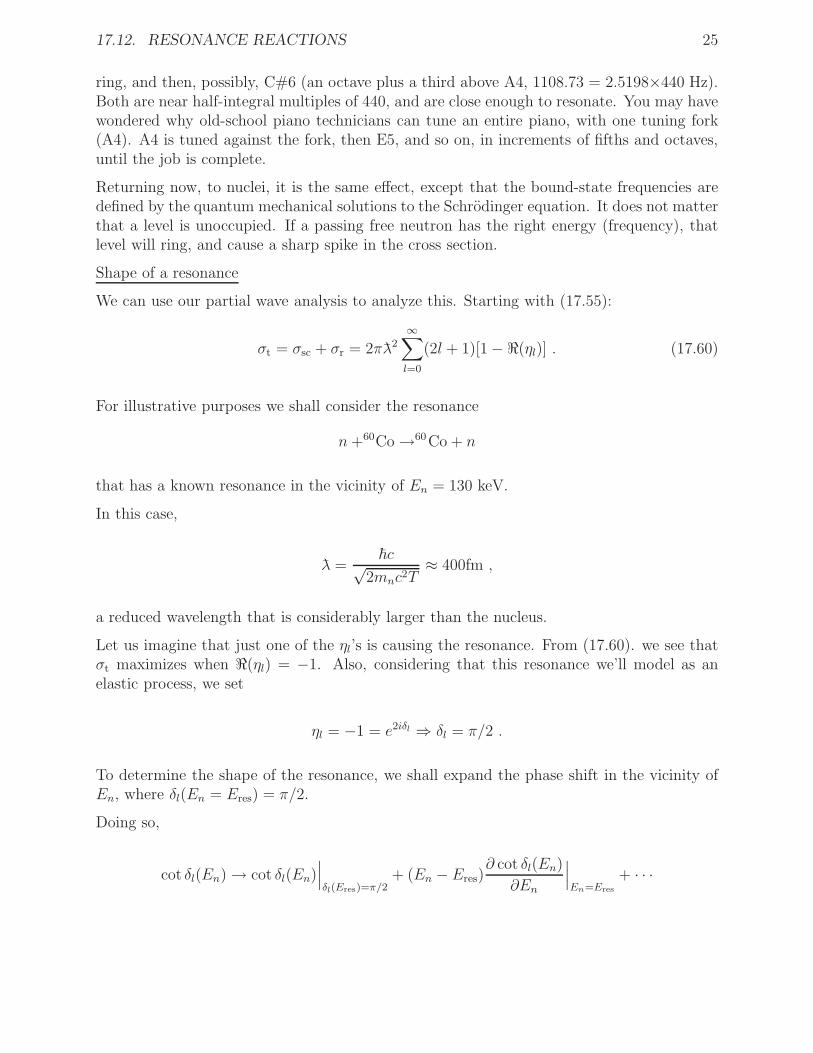
2m(E + V0)/~2. We note that the transmission coefficient is unity, when 2KRis a multiple of π. This is called a resonance. Resonances are depicted in Figure 17.8 forneutrons incident on a potential with depth, V = 40 MeV, and nuclear radius, R = 3.5 fm.Note the dense population of resonant lines. Figure 17.9 isolates only one of these resonances.

In 3 dimensions the analogous thing happens. In fact, it resonances are common everydayoccurrence. All it requires is a bound state that has a given frequency, that can be matchedby an external identical, or nearby frequency. All radios work this way. Unbounded radiowaves are received by antennae that have bound-state frequencies that match. That’s a goodresonance. Good resonances are responsible for a piano’s rich tone. If you look ”underneaththe hood” of a piano, you may have wondered why some hammers hit 3 strings simultane-ously (upper registers), two strings in the middle registers, and one in the bass registers.These nearby strings, grouped at the same pitch, when struck together, cause sympatheticvibrations and overtones that add to the rich sound. Strings of different pitches can interactas well. For example, try the following (on an acoustic piano): Strike A4 (440 Hz the Aabove middle C) quite hard, and then hold down the damper pedal, if your hearing acuityis quite good, you may start to hear E5 (659.26 = 1.4983×440 Hz, a fifth above A4) start to

17.12. RESONANCE REACTIONS 25

ring, and then, possibly, C#6 (an octave plus a third above A4, 1108.73 = 2.5198×440 Hz).Both are near half-integral multiples of 440, and are close enough to resonate. You may havewondered why old-school piano technicians can tune an entire piano, with one tuning fork(A4). A4 is tuned against the fork, then E5, and so on, in increments of fifths and octaves,until the job is complete.

Returning now, to nuclei, it is the same effect, except that the bound-state frequencies aredefined by the quantum mechanical solutions to the Schrodinger equation. It does not matterthat a level is unoccupied. If a passing free neutron has the right energy (frequency), thatlevel will ring, and cause a sharp spike in the cross section.

Shape of a resonance

We can use our partial wave analysis to analyze this. Starting with (17.55):

σt = σsc + σr = 2πλ2∞

∑

l=0

(2l + 1)[1 − ℜ(ηl)] . (17.60)

For illustrative purposes we shall consider the resonance

n+60Co →60Co + n

that has a known resonance in the vicinity of En = 130 keV.

In this case,

λ =~c√

2mnc2T≈ 400fm ,

a reduced wavelength that is considerably larger than the nucleus.

Let us imagine that just one of the ηl’s is causing the resonance. From (17.60). we see thatσt maximizes when ℜ(ηl) = −1. Also, considering that this resonance we’ll model as anelastic process, we set

ηl = −1 = e2iδl ⇒ δl = π/2 .

To determine the shape of the resonance, we shall expand the phase shift in the vicinity ofEn, where δl(En = Eres) = π/2.

Doing so,

cot δl(En) → cot δl(En)∣

∣

∣

δl(Eres)=π/2+ (En − Eres)

∂ cot δl(En)

∂En

∣

∣

∣

En=Eres

+ · · ·


∂ cot δl(En)

∂En= −∂δl(En)

∂En− cos2 δl(En)

sin δl(En)

∂δl(En)

∂En

The second term vanishes above. Defining

Γ = 2

(

∂δl(En)

∂En

)−1∣

∣

∣

En=Eres

,

we have, from the above,

cot δl(En) = −En − Eres

Γ/2, (17.61)

Since,

sin() =1

√

1 + cot2() ,

we have

sin δl =Γ/2

[(En − Eres)2 + Γ2/4]1/2. (17.62)

Finally, combining (17.62) with (17.48)

σelsc(En) = πλ2(2l + 1)

Γ2

[(En − Eres)2 + Γ2/4]. (17.63)

At resonance,

σelassc (En) = 4πλ2(2l + 1) . (17.64)

In this example, λ ≈ 200 fm, giving a resonant cross section of about 200(2l + 1) barns.recalling that the cross section area of a typical nucleus is about 1 b, this is enormous!

What we have calculated so far is only for the case where there is one exit mode for the

a+X −→ X + a

resonance.


Gregory Breit and Eugene Wigner generalized (17.63) as follows:

σelsc(En; [X(a, a)X]) = πλ2 2I + 1

(2sa + 1)(2sX

+ 1)

Γ2aX

[(En − Eres)2 + Γ2/4](17.65)

σinsc(En; [X(a, bi)Yi]) = πλ2 2I + 1

(2sa + 1)(2sX

+ 1)

ΓaXΓbiYi

[(En − Eres)2 + Γ2/4](17.66)

The I in the above equations comes from the coupling of the intrinsic spins of the reactantswith the orbital angular momentum of the outgoing wave component,

~I = ~sX

+ ~sa +~l .

Γ in the denominator of both expressions above, pertains to the sum of all the partial widthsof all the decay modes:

Γ =∑

i

Γi .

The factors ΓaX and ΓbiYiin the above equations, pertain to the partial interaction probabil-

ities for resonance formation, ΓaX and decay, ΓaX , in the case of one of the elastic channels,or ΓbiYi

.

Shape-elastic scattering

Resonant scattering rarely takes place in isolation, but in addition to other continuous elasticscattering, such as Rutherford scattering from a potential. If we call the potential scatteringphase-shift, δP

l , one can show, from (17.47), that:

σsc = πλ2(2l + 1)

∣

∣

∣

∣

e−2δP

l − 1 + iiΓ

(En − Eres) + iΓ/2

∣

∣

∣

∣

2

. (17.67)

Far from the resonance, the resonance dies out, and the cross section has the form:

σsc −→ 4πλ2(2l + 1) sin2 δPl ,

while at the resonance, the resonance dominates and we have:

σsc ≈ 4πλ2(2l + 1) .

In the vicinity of the resonance, the Lorentzian shape is skewed, with a “dip” for E < Eres,that arises from destructive interference between the potential and resonance phases. SeeKrane’s Figures 11.27 and 11.28 for examples of these.


125 126 127 128 129 130 131 132 133 134 1350

0.1

0.2

0.3

0.4

0.5

0.6

0.7

0.8

0.9

1T vs. K

K (eV)

T

Figure 17.8: Resonant structure for an incident neutron. In this case, V0 = 40 MeV, R = 3.5fm.


130.034 130.035 130.036 130.037 130.038 130.039 130.040

0.1

0.2

0.3

0.4

0.5

0.6

0.7

0.8

0.9

1T vs. K

K (eV)

T

Figure 17.9: Resonant structure near one of the peaks.


Problems

1. Derive (17.10).

2. Derive (17.11).

3. Derive (17.14) and (17.15).

4. Work out the derivatives inside the large parentheses in (17.16) and (17.17).

5. Solve the quadratic equation implied by (17.24).

6. Work out Q2 in (17.27).

7. Derive (17.47).

8. Derive (17.48).

9. The screened Rutherford cross section, differential in solid angle, is often used to de-scribe the angular distribution of light charged particles scattering elastically fromheavy nuclei. It has the following form:

dσ

dΩ=

A

(1 − cos θ + a)2,

where A and a are constants for any nucleus-projectile combination. The total crosssection is known to be σ0.

(a) Show that:

A = σ0a(2 + a)

4π.

(b) If the forward (θ = 0) intensity is 106 times greater than that in the backwarddirection (θ = π), show that:

a =2

999.

(c) If the forward (θ = 0) intensity is 4 times greater than that in the backwarddirection (θ = π), Show that:

a = 2 .

(d) In the limit that a −→ ∞, show that the cross section is isotropic.

10. In the X(a, b)Y reaction with known Q and X at rest, it was shown that:

T1/2b =

(mambTa)1/2 cos θ ± mambTa cos2 θ + (mY +mb)[mYQ+ (mY −ma)Ta]1/2

mY +mb

.

Show that:


(a) When Q < 0, there is a minimum value of Ta for which the reaction is not possible.Show that this threshold energy is given by:

Tth = (−Q)mY +mb

mY +mb −ma.

(b) When Q < 0, and Ta > Tth, Tb can take on two values. The maximum Ta thatthis can occur is called T ′

a. Show that:

T ′

a = (−Q)mY

mY −ma.

11. Projectile A, that has mass MA, scatters elastically off of target nucleus X, that hasmass MX . Q = 0, and there is no exchange of matter.

(a) Find a relationship between A’s magnitude of momentum, and its angle of deflec-tion.

(b) Show that there is a maximum scattering angle only when mA > mX .


(c) Find the expression for this maximum angle, when mA > mX .

chapter 17 nuclear reactions - university of michiganners311/courselibrary/bookchapter17.pdf ·...

Documents