chapter 13 stokes' theorem

Stokes’ theorem 1

Chapter 13 Stokes’ theorem

In the present chapter we shall discuss R3 only. We shall use a right-handed coordinatesystem and the standard unit coordinate vectors ı, , k. We shall also name the coordinatesx, y, z in the usual way.

The basic theorem relating the fundamental theorem of calculus to multidimensional in-tegration will still be that of Green. In this chapter, as well as the next one, we shall seehow to generalize this result in two directions. In this chapter we generalize it to surfaces inR3, whereas in the next chapter we generalize to regions contained in Rn. But in all of theseprocedures it is still Green’s theorem that is fundamental.

A. Orientable surfaces

We shall be dealing with a two-dimensional manifold M ⊂ R3. We’ll just use the wordsurface to describe M . There are two features of M that we need to discuss first.

The first is the idea of a normal vector for M . We assume that M is of class C1, so that ateach point p ∈ M there is a vector of unit norm which is orthogonal to M , in the sense thatit is orthogonal to the tangent space TpM . There are of course two choices of such a normalvector, and we now need to make a choice.

DEFINITION. The surface M is said to be orientable if there exists a unit normal vectorN(p) at each point p ∈ M which is a continuous function of p.

The continuity of N(p) is all-important. For instance, one can construct a Mobius stripand obtain a surface which is not orientable:

image createdwith Mathematica ®

In case a surface is described implicitly by an equation

g(x, y, z) = 0

such that∇g is never 0 at any point of the surface, and if g is of class C1, then∇g is continuousand we have two choices for N :

N =∇g

‖∇g‖ or N = − ∇g

‖∇g‖ .

2 Chapter 13

For example, for the ellipsoidx2

a2+

y2

b2+

z2

c2= 1

we may take

N =

(xa2 ,

yb2

, zc2

)√

x2

a4 + y2

b4+ z2

c4

.

For the sphere S(0, a) we have in particular either N

N =(x, y, z)

aor N = −(x, y, z)

a.

REMARK. An orientable surface is also said to be two-sided. The reason for this is thatthe continuous normal vector N serves to define a direction of “up” at points of M . Thus atpoints of M there is a definite sense of two sides of M , an “up” side and a “down” side. AMobius strip for example is one-sided, which may be demonstrated by drawing a curve alongthe “equator” of M with a pencil.

EXTENSION. Frequently we shall need to analyze a surface M ⊂ R3 which is not actuallyorientable in the above sense, but is “close enough.” The surface may consist of finitely manysurfaces with the proper orientability. A few examples should suffice for a good explanation.

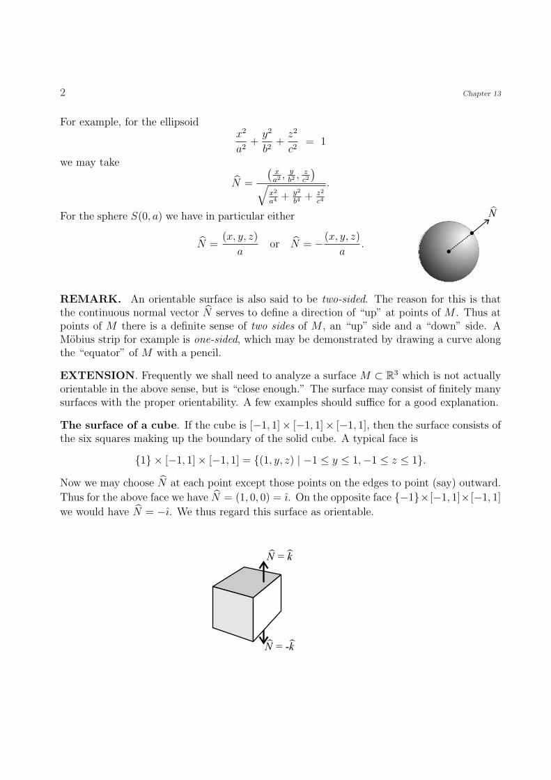
The surface of a cube. If the cube is [−1, 1]× [−1, 1]× [−1, 1], then the surface consists ofthe six squares making up the boundary of the solid cube. A typical face is

{1} × [−1, 1]× [−1, 1] = {(1, y, z) | −1 ≤ y ≤ 1,−1 ≤ z ≤ 1}.Now we may choose N at each point except those points on the edges to point (say) outward.

Thus for the above face we have N = (1, 0, 0) = ı. On the opposite face {−1}×[−1, 1]×[−1, 1]

we would have N = −ı. We thus regard this surface as orientable.

N = k

N = k-

Stokes’ theorem 3

The boundary of a hemiball. For instance consider the hemiball

x2 + y2 + z2 ≤ a2, z ≥ 0.

Then the surface we have in mind consists of the hemisphere

x2 + y2 + z2 = a2, z ≥ 0,

together with the disk

x2 + y2 ≤ a2, z = 0.

If we choose the inward normal vector, then we have

N =(−x,−y,−z)

aon the hemisphere,

N = k on the disk.

A cylindrical can. Consider the surface for which one part is given by

x2 + y2 = a2, 0 ≤ z ≤ h,

and the other part by

x2 + y2 ≤ a2, z = 0.

Then we might choose an “outer” unit normal vector

{N = (x,y,0)

afor 0 < z ≤ h,

N = −k for z = 0.

PROBLEM 13–1. The following surface is orientable. It consists of the union of thecylinder

x2 + y2 = a2, 0 ≤ z ≤ h;

and the hemisphere

x2 + y2 + (z − h)2 = a2, h ≤ z ≤ h + a.

Draw a sketch of it and write down expressions for an “outer” unit normal vector.

4 Chapter 13

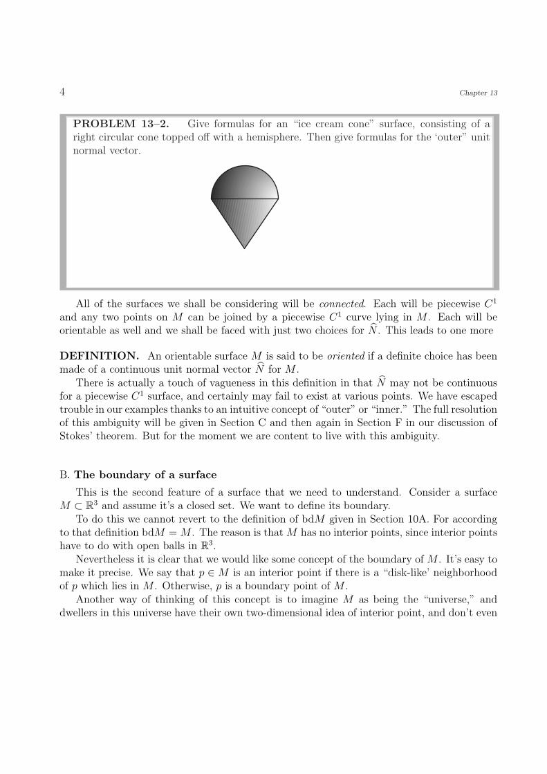
PROBLEM 13–2. Give formulas for an “ice cream cone” surface, consisting of aright circular cone topped off with a hemisphere. Then give formulas for the ‘outer” unitnormal vector.

All of the surfaces we shall be considering will be connected. Each will be piecewise C1

and any two points on M can be joined by a piecewise C1 curve lying in M . Each will beorientable as well and we shall be faced with just two choices for N . This leads to one more

DEFINITION. An orientable surface M is said to be oriented if a definite choice has beenmade of a continuous unit normal vector N for M .

There is actually a touch of vagueness in this definition in that N may not be continuousfor a piecewise C1 surface, and certainly may fail to exist at various points. We have escapedtrouble in our examples thanks to an intuitive concept of “outer” or “inner.” The full resolutionof this ambiguity will be given in Section C and then again in Section F in our discussion ofStokes’ theorem. But for the moment we are content to live with this ambiguity.

B. The boundary of a surface

This is the second feature of a surface that we need to understand. Consider a surfaceM ⊂ R3 and assume it’s a closed set. We want to define its boundary.

To do this we cannot revert to the definition of bdM given in Section 10A. For accordingto that definition bdM = M . The reason is that M has no interior points, since interior pointshave to do with open balls in R3.

Nevertheless it is clear that we would like some concept of the boundary of M . It’s easy tomake it precise. We say that p ∈ M is an interior point if there is a “disk-like’ neighborhoodof p which lies in M . Otherwise, p is a boundary point of M .

Another way of thinking of this concept is to imagine M as being the “universe,” anddwellers in this universe have their own two-dimensional idea of interior point, and don’t even

Stokes’ theorem 5

know about the ambient R3. In other words, they think of intrinsic interior points of M .

NOTATION. The set of boundary points of M will be denoted

∂M.

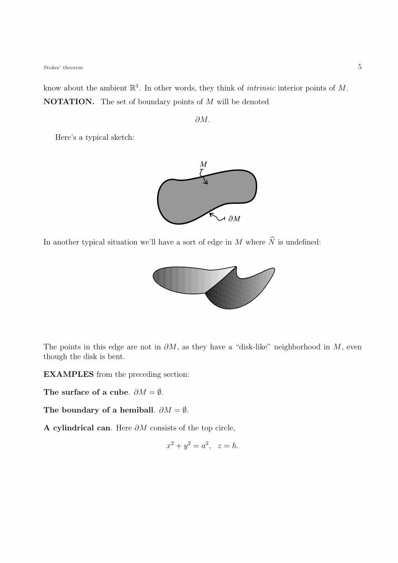
Here’s a typical sketch:

M

M

In another typical situation we’ll have a sort of edge in M where N is undefined:

The points in this edge are not in ∂M , as they have a “disk-like” neighborhood in M , eventhough the disk is bent.

EXAMPLES from the preceding section:

The surface of a cube. ∂M = ∅.

The boundary of a hemiball. ∂M = ∅.

A cylindrical can. Here ∂M consists of the top circle,

x2 + y2 = a2, z = h.

6 Chapter 13

Another typical example is a cylinder “open at both ends”:

M

x2 + y2 = a2,

0 ≤ z ≤ h.

Here ∂M consists of the two circles

x2 + y2 = a2, z = 0 and x2 + y2 = a2, z = h.

DEFINITION. A surface M is closed if ∂M = ∅.Again, this definition conflicts with our use of the same word in Section 10A. Unfortunately,this terminology has become standard. So you must be careful if someone utters the phrase“closed surface.” Be sure you understand what is meant. A better term would be “surfacewithout boundary.”

Typically, if M is equal to bdD for some set D ⊂ R3, then M is a closed surface.Notice that ∂M may consist of several disjoint arcs.

C. Inherited orientation

The two concepts of orientation and boundary have an important relationship. Namely,suppose the oriented surface M has a nonempty boundary ∂M . Consider an arc belongingto ∂M . Then we can assign a direction to ∂M by saying that if we walk along ∂M with ourheads “up,” then we see M at our left sides. Of course “up” refers to the chosen unit normalvector N .

We describe this by saying that ∂M inherits its orientation from M .Notice that this is in complete agreement with our statement of Green’s theorem. There

bdR is given the direction which keeps R on the left, if we suppose a third z direction pointing“up” from the x− y plane with its usual orientation.

Stokes’ theorem 7

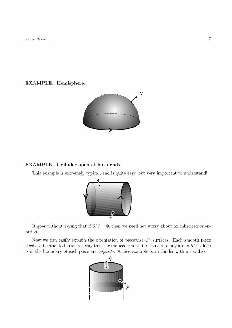
EXAMPLE. Hemisphere.

N

EXAMPLE. Cylinder open at both ends.

This example is extremely typical, and is quite easy, but very important to understand!

It goes without saying that if ∂M = ∅, then we need not worry about an inherited orien-tation.

Now we can easily explain the orientation of piecewise C1 surfaces. Each smooth pieceneeds to be oriented in such a way that the induced orientations given to any arc in ∂M whichis in the boundary of each piece are opposite. A nice example is a cylinder with a top disk:

N

N

8 Chapter 13

The displayed unit normal vectors N give opposite orientations to the circular arc the twoparts of the surface have in common.

D. The basic calculation

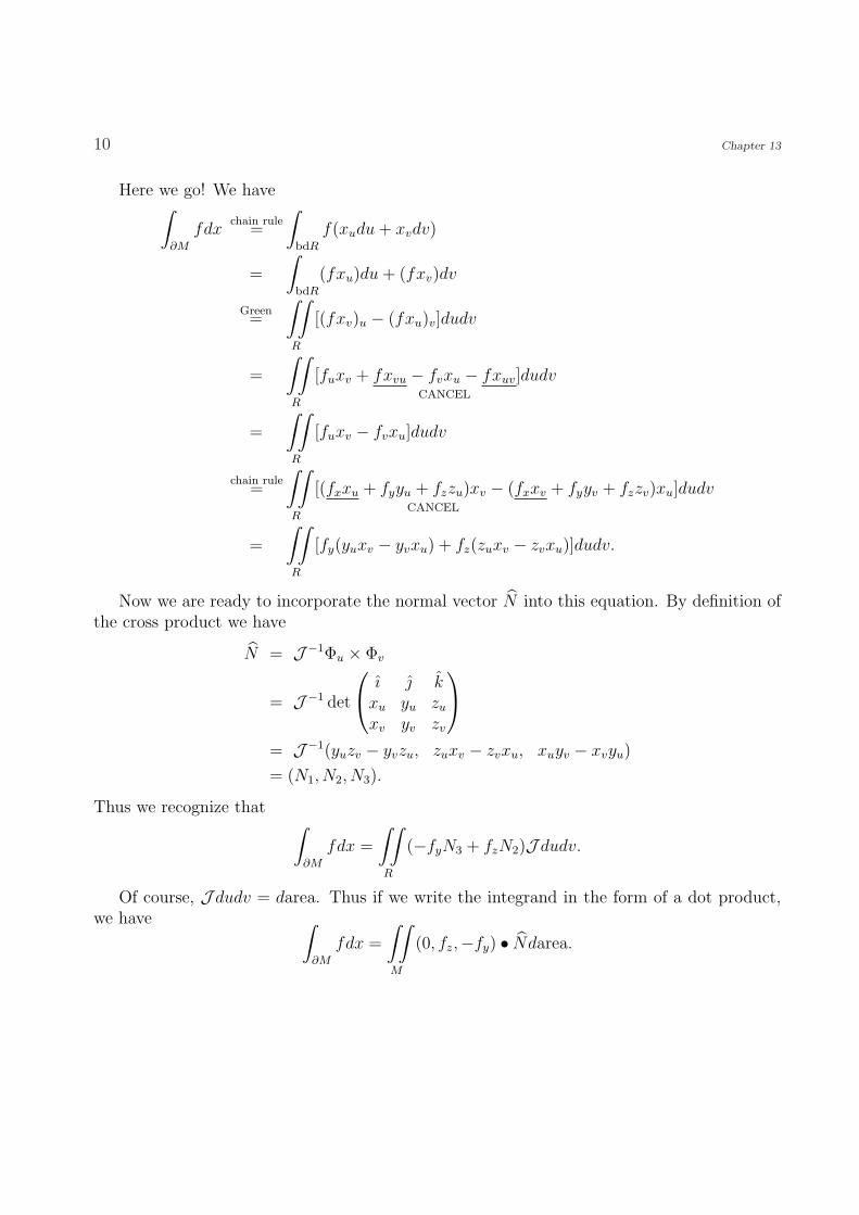
Now we are ready to go! We start with a small piece of an oriented surface, and we actuallyassume it’s of class C2. Call it M ⊂ R3. This surface is to be considered to be parameterizedin the usual way. Let us call the parameters u, v, so we have a parameter mapping Φ from aregion R ⊂ R2 onto M .

R

MR

M

We know that the partial derivatives Φu, Φv give a basis for the tangent space to M atany point, and thus their cross product Φu × Φv is a nonzero vector normal to M . As M isoriented we are given a unit normal vector N at each point of M . We now want to makesure that Φu × Φv is a positive scalar multiple of M . This can be achieved by the device ofinterchanging u and v if necessary. Thus we have

N =Φu × Φv

J ,

where the denominator J is simply the norm

J = ‖Φu × Φv‖.

From Section 11B we know that area integration on M comes from J as the Jacobianfactor:

darea = J dudv.

Next, we make sure that we represent the parameter u − v space as a right-handed coor-dinate system, as shown in the figure. Then we make the all-important observation that the

Stokes’ theorem 9

positive direction of bdR in the parameter space corresponds to the inherited orientation of∂M in R3. You should check this for yourself:

PROBLEM 13–3. Prove the statement just made about the orientation.

Now we are ready for the computation. The goal we have in mind is to rewrite a generalline integral of the form ∫

∂M

F • d~x

as a surface integral of the form ∫∫

M

(???)darea.

(We don’t yet know what the integrand will be.) In doing this we have to integrate along ∂M

in the direction inherited from N . We need a parameter for describing ∂M , and we’ll just usea convenient parameter t for describing bdR. That is, bdR may be described by functionsu = u(t), v = v(t), and then ∂M is described by the three coordinates

x = x(u(t), v(t)),

y = y(u(t), v(t)),

z = z(u(t), v(t)).

Here we abuse the notation by thinking of Φ as described by three functions x = x(u, v),y = y(u, v), z = z(u, v). But we’ll completely suppress t in our calculation. You’ll never needto see it.

Please notice that we write our surface integrals in the present chapter with two integralsigns, as the manifolds we consider are always two-dimensional ones (and their one-dimensionalboundaries).

Finally, we shall calculate just the particular special case of our line integrals,

∫

∂M

fdx.

In other words, F = (f, 0, 0). We’ll then easily get the other two cases by cycling through theindices.

10 Chapter 13

Here we go! We have∫

∂M

fdxchain rule

=

∫

bdR

f(xudu + xvdv)

=

∫

bdR

(fxu)du + (fxv)dv

Green=

∫∫

R

[(fxv)u − (fxu)v]dudv

=

∫∫

R

[fuxv + fxvu − fvxu − fxuv

CANCEL

]dudv

=

∫∫

R

[fuxv − fvxu]dudv

chain rule=

∫∫

R

[(fxxu + fyyu + fzzu)xv − (fxxv

CANCEL

+ fyyv + fzzv)xu]dudv

=

∫∫

R

[fy(yuxv − yvxu) + fz(zuxv − zvxu)]dudv.

Now we are ready to incorporate the normal vector N into this equation. By definition ofthe cross product we have

N = J −1Φu × Φv

= J −1 det

ı kxu yu zu

xv yv zv

= J −1(yuzv − yvzu, zuxv − zvxu, xuyv − xvyu)

= (N1, N2, N3).

Thus we recognize that∫

∂M

fdx =

∫∫

R

(−fyN3 + fzN2)J dudv.

Of course, J dudv = darea. Thus if we write the integrand in the form of a dot product,we have ∫

∂M

fdx =

∫∫

M

(0, fz,−fy) • Ndarea.

Stokes’ theorem 11

This is the end result of our calculation. The parameters have disappeared and everything isin terms of the surface M .

It is truly wonderful that just knowing the flat Green’s theorem has led to this curvedversion by just routine manipulations of the definitions. Almost no thought was required!

“I cast it into the fire, and there came out this calf”−Aaron, Exodus 3224

E. The basic theorem, curl

We now very quickly extend the result we have just proved by cycling through the coordi-nates x → y → z → x. Thus we must have∫

∂M

gdy =

∫∫

M

(−gz, 0, gx) • Ndarea

and ∫

∂M

hdz =

∫∫

M

(hy,−hx, 0) • Ndarea.

We then add our three basic line integrals to obtain∫

∂M

fdx + gdy + hdz =

∫∫

M

(hy − gz, fz − hx, gx − fy) • Ndarea.

We have come to a point where we need to make a fascinating

DEFINITION. Given a vector field F = (f, g, h) of class C1 on R3, the curl of F is thevector field

curlF = (hy − gz, fz − hx, gx − fy).

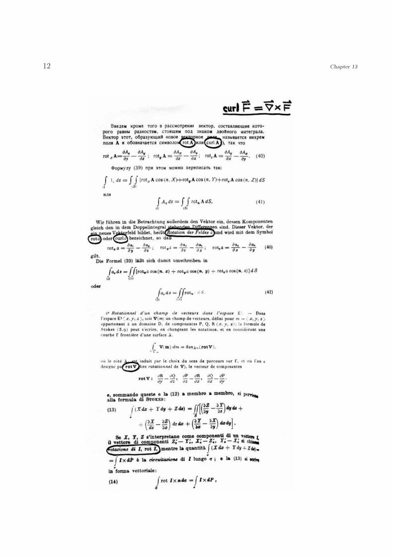
Incidentally, most languages other than English use the word rotation in place of curl,and write rotF for the vector field. On the next page you will find examples that have beenphotocopied from calculus texts in Russian, German, French, and Italian.

This vector field curlF is quite amazing. You should keep in mind how very naturally itappeared in our calculations. It isn’t something we had to be clever to invent; it simply arosein the calculations.

There’s a wonderful mnemonic for the curl. Recall the mnemonic for the cross product oftwo vectors,

a× b = det

ı ka1 a2 a3

b1 b2 b3

,

12 Chapter 13


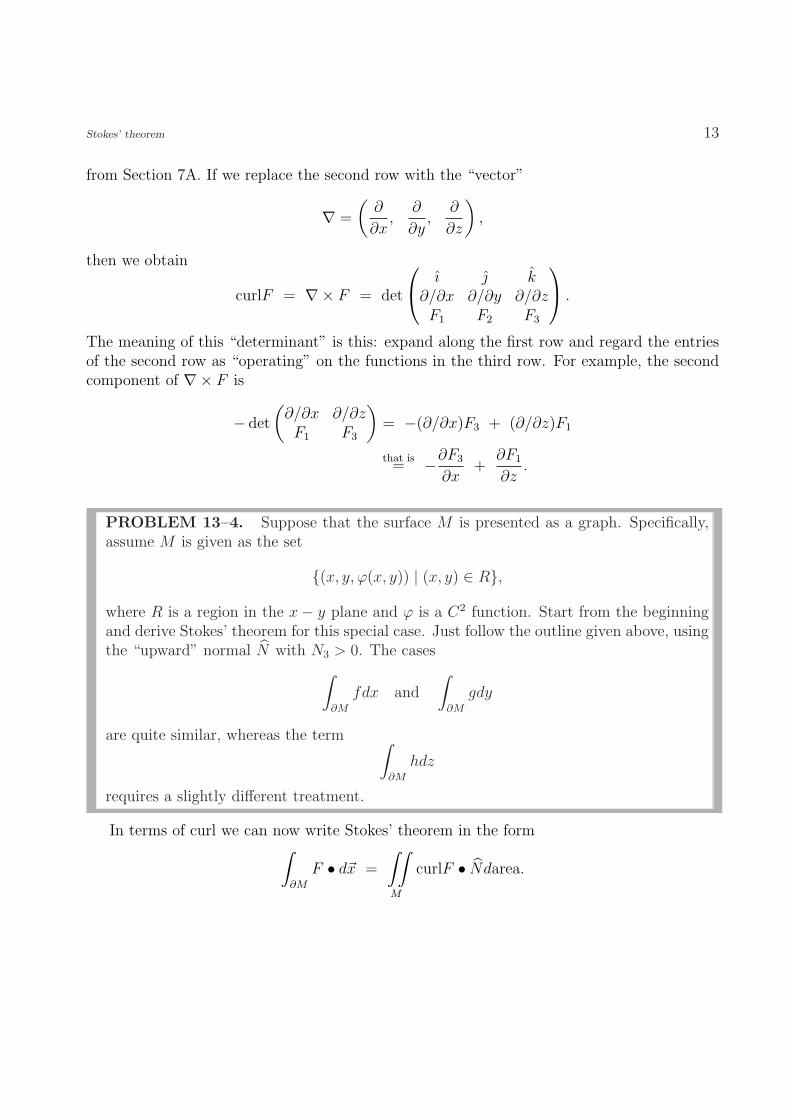
from Section 7A. If we replace the second row with the “vector”

∇ =

(∂

∂x,

∂

∂y,

∂

∂z

),

then we obtain

curlF = ∇× F = det

ı k∂/∂x ∂/∂y ∂/∂zF1 F2 F3

.

The meaning of this “determinant” is this: expand along the first row and regard the entriesof the second row as “operating” on the functions in the third row. For example, the secondcomponent of ∇× F is

− det

(∂/∂x ∂/∂zF1 F3

)= −(∂/∂x)F3 + (∂/∂z)F1

that is= −∂F3

∂x+

∂F1

∂z.

PROBLEM 13–4. Suppose that the surface M is presented as a graph. Specifically,assume M is given as the set

{(x, y, ϕ(x, y)) | (x, y) ∈ R},

where R is a region in the x− y plane and ϕ is a C2 function. Start from the beginningand derive Stokes’ theorem for this special case. Just follow the outline given above, usingthe “upward” normal N with N3 > 0. The cases

∫

∂M

fdx and

∫

∂M

gdy

are quite similar, whereas the term ∫

∂M

hdz

requires a slightly different treatment.

In terms of curl we can now write Stokes’ theorem in the form∫

∂M

F • d~x =

∫∫

M

curlF • Ndarea.

14 Chapter 13

This is our basic version of Stokes’ theorem. Now we show how to extend it.

F. Stokes’ theorem

We have proved the result in the preceding section under the restrictive hypothesis thatM is presented in terms of a single parametrization. We now go through the same exerciseswe used in Section 12C to extend Green’s theorem.

The fundamental observation is in fact the same we used for Green. If two pieces of Mmeet along a seam and Stokes is applied to each, the line integrals along the seam cancel eachother because of our assumption on the orientation of M and the inherited orientation of ∂M .Here’s a sketch:

M1

M2

We then can finally present our theorem as follows:

STOKES’ THEOREM. Assume M is a piecewise C2 bounded oriented surface in R3 whoseboundary ∂M has the inherited orientation. Assume F is a C1 vector field defined on M . Then

∫

∂M

F • d~x =

∫∫

M

curlF • Ndarea.

In summary, Stokes’ theorem may be regarded precisely as a curved version of Green’stheorem in the plane.

Important special case: In the above theorem, if M is a closed surface (∂M = ∅), then

∫∫

M

curlF • Ndarea = 0.


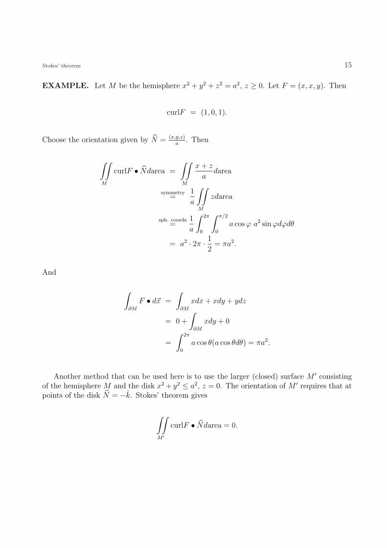
EXAMPLE. Let M be the hemisphere x2 + y2 + z2 = a2, z ≥ 0. Let F = (x, x, y). Then

curlF = (1, 0, 1).

Choose the orientation given by N = (x,y,z)a

. Then

∫∫

M

curlF • Ndarea =

∫∫

M

x + z

adarea

symmetry=

1

a

∫∫

M

zdarea

sph. coords=

1

a

∫ 2π

0

∫ π/2

0

a cos ϕ a2 sin ϕdϕdθ

= a2 · 2π · 1

2= πa2.

And

∫

∂M

F • d~x =

∫

∂M

xdx + xdy + ydz

= 0 +

∫

∂M

xdy + 0

=

∫ 2π

0

a cos θ(a cos θdθ) = πa2.

Another method that can be used here is to use the larger (closed) surface M ′ consistingof the hemisphere M and the disk x2 + y2 ≤ a2, z = 0. The orientation of M ′ requires that atpoints of the disk N = −k. Stokes’ theorem gives

∫∫

M ′

curlF • Ndarea = 0.

16 Chapter 13

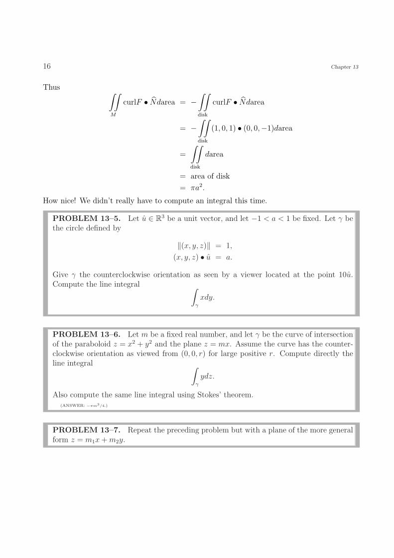
Thus ∫∫

M

curlF • Ndarea = −∫∫

disk

curlF • Ndarea

= −∫∫

disk

(1, 0, 1) • (0, 0,−1)darea

=

∫∫

disk

darea

= area of disk

= πa2.

How nice! We didn’t really have to compute an integral this time.

PROBLEM 13–5. Let u ∈ R3 be a unit vector, and let −1 < a < 1 be fixed. Let γ bethe circle defined by

‖(x, y, z)‖ = 1,

(x, y, z) • u = a.

Give γ the counterclockwise orientation as seen by a viewer located at the point 10u.Compute the line integral ∫

γ

xdy.

PROBLEM 13–6. Let m be a fixed real number, and let γ be the curve of intersectionof the paraboloid z = x2 + y2 and the plane z = mx. Assume the curve has the counter-clockwise orientation as viewed from (0, 0, r) for large positive r. Compute directly theline integral ∫

γ

ydz.

Also compute the same line integral using Stokes’ theorem.(ANSWER: −πm3/4.)

PROBLEM 13–7. Repeat the preceding problem but with a plane of the more generalform z = m1x + m2y.


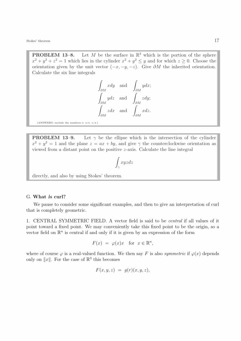
PROBLEM 13–8. Let M be the surface in R3 which is the portion of the spherex2 + y2 + z2 = 1 which lies in the cylinder x2 + y2 ≤ y and for which z ≥ 0. Choose theorientation given by the unit vector (−x,−y,−z). Give ∂M the inherited orientation.Calculate the six line integrals

∫

∂M

xdy and

∫

∂M

ydx;∫

∂M

ydz and

∫

∂M

zdy;∫

∂M

zdx and

∫

∂M

xdz.

(ANSWERS: include the numbers 0, 2/3, π/4.)

PROBLEM 13–9. Let γ be the ellipse which is the intersection of the cylinderx2 + y2 = 1 and the plane z = ax + by, and give γ the counterclockwise orientation asviewed from a distant point on the positive z-axis. Calculate the line integral

∫

γ

xyzdz

directly, and also by using Stokes’ theorem.

G. What is curl?

We pause to consider some significant examples, and then to give an interpretation of curlthat is completely geometric.

1. CENTRAL SYMMETRIC FIELD. A vector field is said to be central if all values of itpoint toward a fixed point. We may conveniently take this fixed point to be the origin, so avector field on Rn is central if and only if it is given by an expression of the form

F (x) = ϕ(x)x for x ∈ Rn,

where of course ϕ is a real-valued function. We then say F is also symmetric if ϕ(x) dependsonly on ‖x‖. For the case of R3 this becomes

F (x, y, z) = g(r)(x, y, z),

18 Chapter 13

where of course r = ‖(x, y, z)‖ is the usual spherical coordinate. Then for example the firstcomponent of curlF equals

∂

∂y(g(r)z)− ∂

∂z(g(r)y) = g′(r)

yz

r− g′(r)

zy

r

= 0.

Thus curlF = 0.

2. CONSERVATIVE FIELD. Our definition from Section 12 states that a vector field on R3

is conservative if there exists a potential function f such that F = ∇f . Assuming that f is ofclass C2, we conclude that curlF = 0. For instance, the second coordinate of curlF is

∂F1

∂z− ∂F3

∂x=

∂

∂z

∂f

∂x− ∂

∂x

∂f

∂z= 0.

Thus we have the interesting result, that always

curl gradf = 0.

Or in terms of the “del” notation,∇×∇f = 0.

3. REMARK. Actually, Example 1 is a special case of Example 2, as every central symmetricfield is conservative. This is even true for Rn. For suppose

F (x) = ϕ(r)x

is given on Rn, and we want to find a potential function for F . We would certainly expectthis potential to be spherically symmetric itself, so we look for a function of the form f(r).We thus want

∇(f(r)) = ϕ(r)x;

that is,

f ′(r)x

r= ϕ(r)x;

we thus simply need to integrate the equation

f ′(r) = rϕ(r)

in order to find f .


4. ZERO CURL. We now can explain the strange terminology of Section 12E. There we saidthat a vector field F on Rn with

∂Fi

∂xj

=∂Fj

∂xi

has zero curl. In case n = 3 this is exactly the condition that curlF = 0, so by analogy wesay the same for general n. It’s just that for n 6= 3 we don’t actually have a vector field wecall curlF .

5. PLANAR FIELDS. Suppose a vector field on R3 has the special form

F (x, y, z) = (F1(x, y), F2(x, y), 0),

so that F is parallel to the plane z = 0 and also is independent of z. Then

curlF =

(∂F2

∂x− ∂F1

∂y

)k.

6. EXAMPLES OF PLANAR FIELDS. Our first example comes from the famous ∇θ on R2,so that

F =

( −y

x2 + y2,

x

x2 + y2, 0

).

Then curlF = 0. Two more significant examples are

curl(−y, x, 0) = 2k,

curl(y, 0, 0) = −k.

PROBLEM 13–10. Let a ∈ R3 be an arbitrary fixed vector. Show that

∇× (a× ~x) = 2a.

(Here ~x stands for (x, y, z).)

PROBLEM 13–11. The vector field a × ~x of the preceding problem is a special caseof a general linear vector field. Such a field can be written F (~x) = A~x, where A is a real3× 3 matrix and ~x is written as a column vector. Show that

∇× F = (a32 − a23, a13 − a31, a21 − a12).

20 Chapter 13

PROBLEM 13–12. Here is a problem from American Mathematical Monthly, Volume 109, Number 7, August-

September, 2002, proposed by Victor Alexandrov, Sobolev Institute of Mathematics, Novosibirsk, Russia:Let M be a surface contained in the unit sphere in R3. Use the outer unit normal

vector N for the sphere. In addition, let n denote the unit vector at points of ∂M whichis tangent to the unit sphere and is orthogonal to ∂M . (In particular, n • N = 0.) Provethat ∫

∂M

nds + 2

∫∫

M

Ndarea = 0.

Here ds denotes arc length and the integrals with vector integrands are to be interpretedin the sense of integrating the components and then combining the results into vectors.(HINT: apply Stokes to the vector field F = a× ~x for any fixed vector a.)


PROBLEM 13–13. Let C denote the unit circle

{(x, y, 0) | x2 + y2 = 1}

in R3. Define the “function” g on R3 − C by

g(x, y, z) = arctanz

x2 + y2 − 1.

Of course, g is not completely well defined.

a. Prove that the vector field F = ∇g is a well defined vector field on R3 − C, andthat it is C∞.

b. Prove that F is irrotational.

c. Prove that F is not conservative by showing that there is a loop in R3 − C alongwhich the line integral of F is not zero.

d. Calculate F explicitly, and show that on the specific loop γ

y = 0, z2 = 2x2 − x4 (x ≥ 0),

the line integral of F equals

∫

γ

−2xzdx + (x2 − 1)dz.

Calculate this integral directly and show it equals 2π.

GEOMETRY. We now present a geometric interpretation of curl which provides intuitionfor the above examples and others. First, we need to understand line integrals in a certaingeometric way. Suppose that F is a vector field on Rn and γ is a curve in Rn, say γ = γ(t),a ≤ t ≤ b. Then the dot product

F (γ(t)) • γ′(t)

represents the component of F in the direction tangent to the curve, multiplied by the speedof the curve. Thus in a very significant sense the integral

∫ b

a

F (γ(t)) • γ′(t)dt

22 Chapter 13

represents the total net component of F tangent to the curve γ. In particular, if γ is a closedcurve, then this integral represents the net increase of the tangential component of F aroundγ. We thus say that

∫

γ

F • d~x = the net circulation of F around γ.

In case F represents a force, then we might think of the circulation as the net work doneby F in going around γ. In case F represents the velocity of a fluid, then it would be the netflow of the fluid.

In particular, a vector field is conservative ⇐⇒ it has zero circulation around every closedcurve.

PROBLEM 13–14. Let F be a vector field in R2 which is given by

F = rα(−y, x). (r =√

x2 + y2)

Find the net circulation of F around the counterclockwise circle x2 + y2 = a2. For whichvalue of α is the result independent of the radius a?

Stokes’ theorem thus asserts that in the case of R3 the net circulation of F around ∂Mmay be measured by calculating the surface integral over M of the normal component of thecurl of F (with proper orientation).

This idea may be presented infinitesimally in such a way as to give an entirely differentway of defining curl. To see this, suppose F is a vector field on R2 which is defined in someneighborhood of a fixed point p0. We shall derive a formula for curlF (p0) without using anycoordinate system and even without using any partial derivatives of any components of F !

In order to know curlF (p0), it suffices to know the number curlF (p0)• u for any unit vectoru. This dot product is of course the component of the vector curlF (p0) in the direction u.Construct the disk Dε with center p0, radius ε, orthogonal to u.

Use the vector u as the unit normal vector for Dε, thus rendering Dε an oriented surface. Thebounding circle ∂Dε is of course supplied with the induced orientation: it travels counterclock-


wise as viewed from the tip of u. Then Stokes’ theorem gives

∫∫

Dε

curlF • udarea =

∫∫

∂Dε

F • d~x.

If ε is small, the left side of this equation is very close to curlF (p0) • u times the area of Dε,thanks to the continuity of the integrand. Thus if we divide by πε2 and let ε → 0, we obtain

curlF (p0) • u = limε→0

1

πε2

∫

∂Dε

F • d~x.

There is a significant way to think about the right side of this equation in terms of the ideaof circulation, and this lead to the sentence

curlF (p0) • u = “the counterclockwise circulation per unit area of F at p0 with respect to u.”

MORAL. The right sides of these expressions have a definite meaning independent of anychoice of coordinate system. Thus the same must be true of curlF (p0) • u. As this is true forevery choice of the unit vector u, we conclude that

the curl of a vector field on R3 is a geometric property of the field, depending onlyon the choice of the orientation of R3.

Notice how very naturally this description of curl has arisen. Natural as it is, it is neverthelessstunning in view of our initial definition in terms of the coordinate system,

curl(F1ı + F2 + F3k) = det

ı k∂/∂x ∂/∂y ∂/∂zF1 F2 F3

.

All three rows of the matrix depend on the coordinate system, but the output does not!Once again we observe the wonderful interplay between algebra and geometry! Stokes’

theorem provides us with the deep geometric significance of curl, while the initial definitiongives us a handy way of computing the curl of vector field.

For instance, suppose {φ1, φ2, φ3} is a right-handed orthonormal frame for R3 and definecoordinates t1, t2, t3 by the formula

(x, y, z) = t1φ1 + t2φ2 + t3φ3.

24 Chapter 13

Then we conclude immediately that

curlF = det

φ1 φ2 φ3

∂/∂t1 ∂/∂t2 ∂/∂t3F • φ1 F • φ2 F • φ3

.

No calculations needed!

PROBLEM 13–15. How does this formula change if {φ1, φ2, φ3} is a left-handedorthonormal frame?

This is a good time to remember that we stressed a similar geometry/algebra connectionback in Section 2H in our discussion of the gradient of a function. We thus arrive at twosignificant geometric insights into the “differential operator” ∇ = (∂/∂x, ∂/∂y, ∂/∂z), onewhen it acts on functions to produce conservative vector fields ∇f , and now one when it actson vector fields to produce new vector fields ∇× F .

You should also notice why curlF is also called the rotation of F and is sometimes writtenrotF , as we mentioned in Section E. It all has to do with the geometric description of curl interms of the circulation, or rotation, of the vector field.

There are some straightforward calculus results that are frequently quite helpful in manip-ulating curl. We have seen one already: ∇×∇f = 0. Here is a useful product rule:

PROBLEM 13–16. Show that

∇× (fF ) = f∇× F +∇f × F.

In Chapter 15 we shall greatly extend the formula given above for curlF to allow nonorthog-onal frames, and in fact to allow curvilinear coordinates.

H. Curlometer

Imagine a fluid flowing in R3, and imagine the velocity vector at each point ~x. This givessome sort of a vector field F (~x), which we suppose to be independent of time.

The streamlines of this fluid are obtained by solving the system of ordinary differentialequations for the curves ~x(t):

d~x

dt= F (~x(t)).


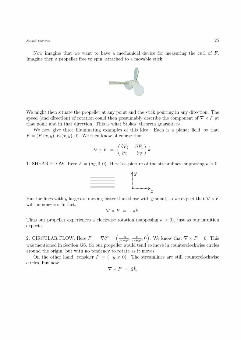
Now imagine that we want to have a mechanical device for measuring the curl of F .Imagine then a propeller free to spin, attached to a movable stick:

We might then situate the propeller at any point and the stick pointing in any direction. Thespeed (and direction) of rotation could then presumably describe the component of ∇× F atthat point and in that direction. This is what Stokes’ theorem guarantees.

We now give three illuminating examples of this idea. Each is a planar field, so thatF = (F1(x, y), F2(x, y), 0). We then know of course that

∇× F =

(∂F2

∂x− ∂F1

∂y

)k.

1. SHEAR FLOW. Here F = (ay, 0, 0). Here’s a picture of the streamlines, supposing a > 0.

But the lines with y large are moving faster than those with y small, so we expect that ∇×Fwill be nonzero. In fact,

∇× F = −ak.

Thus our propeller experiences a clockwise rotation (supposing a > 0), just as our intuitionexpects.

2. CIRCULAR FLOW. Here F = “∇θ” =(

−yx2+y2 ,

xx2+y2 , 0

). We know that ∇× F = 0. This

was mentioned in Section G6. So our propeller would tend to move in counterclockwise circlesaround the origin, but with no tendency to rotate as it moves.

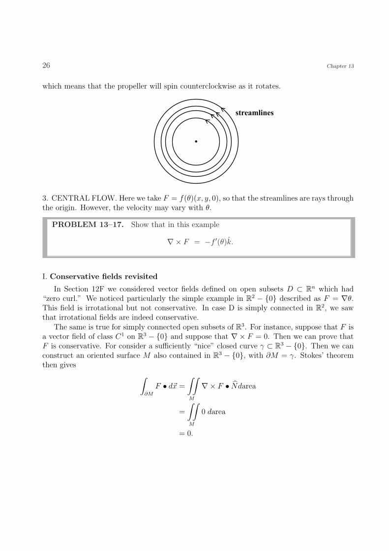
On the other hand, consider F = (−y, x, 0). The streamlines are still counterclockwisecircles, but now

∇× F = 2k,

26 Chapter 13

which means that the propeller will spin counterclockwise as it rotates.

streamlines

3. CENTRAL FLOW. Here we take F = f(θ)(x, y, 0), so that the streamlines are rays throughthe origin. However, the velocity may vary with θ.

PROBLEM 13–17. Show that in this example

∇× F = −f ′(θ)k.

I. Conservative fields revisited

In Section 12F we considered vector fields defined on open subsets D ⊂ Rn which had“zero curl.” We noticed particularly the simple example in R2 − {0} described as F = ∇θ.This field is irrotational but not conservative. In case D is simply connected in R2, we sawthat irrotational fields are indeed conservative.

The same is true for simply connected open subsets of R3. For instance, suppose that F isa vector field of class C1 on R3 − {0} and suppose that ∇× F = 0. Then we can prove thatF is conservative. For consider a sufficiently “nice” closed curve γ ⊂ R3 − {0}. Then we canconstruct an oriented surface M also contained in R3 − {0}, with ∂M = γ. Stokes’ theoremthen gives

∫

∂M

F • d~x =

∫∫

M

∇× F • Ndarea

=

∫∫

M

0 darea

= 0.


This verifies the validity of the second criterion in the theorem of Section 12E, and thus F isconservative.

The reason for the difference between R2−{0} and R3−{0} is clear: in R3−{0} there isroom to maneuver to fill in a loop with a surface missing the origin.

PROBLEM 13–18. Show that the same result holds for the open set

R3 − R× [0,∞)× {0}.

chapter 13 stokes' theorem

Documents