chapter 12 solutions - home | department of statistics | …ghobbs/stat511hw/ips6e.ism.ch1… ·...

Chapter 12 Solutions

12.1. (a) H0 says the population means are all equal. (b) Experiments are best for establishingcausation. (c) ANOVA is used when the explanatory variable has two or more values.

12.2. (a) If we reject H0, we conclude that at least one mean is different from the rest.(b) There is no theoretical limit to the number of means that can be compared. (c) Two-wayANOVA is used to examine the effect of two explanatory variables on a response variable.

12.3. We were given sample sizes n1 = 25, n2 = 22, and n3 = 19 and standard deviationss1 = 22, s2 = 20, and s3 = 18. (a) Yes: The guidelines for pooling standard deviationssay that the ratio of largest to smallest should be less than 2; we have 22

18.= 1.22 < 2.

(b) Squaring the three standard deviations gives s21 = 484, s2

2 = 400, and s23 = 324.

(c) s2p = 24s2

1 + 21s22 + 18s2

3

24 + 21 + 18.= 410.2857. (d) sp =

√s2p

.= 20.2555.

12.4. These pictures are shown below. Note that for (b), there are four curves, but two coincidealmost exactly (one centered at 20, the other at 20.1).

(a) (b) (c)

18 24 30 3660 12 15 20 255 10

twocurves

1510 2520

12.5. (a) This sentence describes between-group variation. Within-group variation is thevariation that occurs by chance among members of the same group. (b) The sum of squares(not the mean squares) in an ANOVA table will add. (c) The common population standarddeviation σ (not its estimate sp) is a parameter.

12.6. The answers are found in Table E (or using software) with p = 0.05 and degrees offreedom I − 1 and N − I . (a) I = 5, N = 15, df 4 and 10: F > 3.48 (software: 3.4781).(b) I = 5, N = 30, df 4 and 25: F > 2.76 (software: 2.7587). (c) I = 5, N = 45, df 4and 40: F > 2.61 (software: 2.6060). (d) As the degrees of freedom increase, values froman F distribution tend to be smaller (closer to 1), so smaller values of F are statisticallysignificant. In terms of ANOVA conclusions, we have learned that with smaller samples(fewer observations per group), the F statistic needs to be fairly large in order to reject H0.

12.7. Assuming the t (ANOVA) test establishes that the means are different, contrasts andmultiple comparison provide no further useful information. (With two means, there is onlyone comparison to make, and it has already been made by the t test.)

12.8. (a) The stated hypothesis is µ50% < 12(µ0% + µ100%), so we use the contrast

ψ = 12(µ0% + µ100%) − µ50%, with coefficients 0.5, −1, and 0.5. The hypotheses

can then be stated H0: ψ = 0 vs. Ha: ψ > 0. (b) The estimated contrast is

c = 12(50 + 120) − 75 = 10 cm3, with standard error SEc = sp

√0.2540 + 1

40 + 0.2540

.= 5.8095, so

324

Solutions 325

the test statistic is t.= 10

5.8095.= 1.7213 with df = 117. The one-sided P-value is P = 0.0439,

so this is significant at α = 0.05, but not at α = 0.05.Note: We wrote the contrast so that it would be positive when Ha is true (in

keeping with the text’s advice). We could also test this hypothesis using the contrastψ ′ = µ50% − 1

2(µ0% + µ100%), or even ψ ′′ = µ0% + µ100% − 2µ50%. The resulting t statisticis the same (except possibly in sign) regardless of the way the contrast is stated.

12.9. (a) Response: egg cholesterol level. Populations: chickens with different diets or drugs.I = 3, n1 = n2 = n3 = 25, N = 75. (b) Response: rating on five-point scale. Populations:the three groups of students. I = 3, n1 = 31, n2 = 18, n3 = 45, N = 94. (c) Response: quizscore. Populations: students in each TA group. I = 3, n1 = n2 = n3 = 14, N = 42.

12.10. (a) Response: time to complete VR path. Populations: children using differentnavigation methods. I = 4, ni = 10 (i = 1, 2, 3, 4), N = 40. (b) Response:calcium content of bone. Populations: chicks eating diets with differing pesticide levels.I = 5, ni = 13 (i = 1, 2, 3, 4, 5), N = 65. (c) Response: total sales between 11:00 a.m.and 2:00 p.m. Populations: customers responding to one of four sample offers. I = 4,ni = 5 (i = 1, 2, 3, 4) and N = 20.

12.11. For all three situations, the hypotheses are H0: µ1 = µ2 = µ3 vs. Ha: at least onemean is different. The degrees of freedom are DFG = DFM = I − 1 (“model” or “betweengroups”), DFE = DFW = N − I (“error” or “within groups”), and DFT = N − 1 (“total”).The degrees of freedom for the F test are DFG and DFE.

Situation I N DFG DFE DFT df for F statisticEgg cholesterol level 3 75 2 72 74 F(2, 72)

Student opinions 3 94 2 91 93 F(2, 91)

Teaching assistants 3 42 2 39 41 F(2, 39)

12.12. For all three situations, the hypotheses are H0: µ1 = µ2 = · · · = µI vs. Ha: at least onemean is different. The degrees of freedom are DFG = DFM = I − 1 (“model” or “betweengroups”), DFE = DFW = N − I (“error” or “within groups”), and DFT = N − 1 (“total”).The degrees of freedom for the F test are DFG and DFE.

Situation I N DFG DFE DFT df for F statisticVR navigation methods 4 40 3 36 39 F(3, 36)

Effect of pesticide on birds 5 65 4 60 64 F(4, 60)

Effect of free food on sales 4 20 3 16 19 F(3, 16)

12.13. (a) This sounds like a fairly well designed experiment, so the results should at leastapply to this farmer’s breed of chicken. (b) It would be good to know what proportion ofthe total student body falls in each of these groups—that is, is anyone overrepresented inthis sample? (c) How well a TA teaches one topic (power calculations) might not reflect thatTA’s overall effectiveness.

326 Chapter 12 One-Way Analysis of Variance

12.14. (a) This sounds like a fairly well designed experiment, assuming the subjects comefrom a group which is representative of the population. (We assume that this teaching tool isintended for use with children and that the children used in the experiment were themselvesdeaf.) (b) This should at least give information about pesticide effect on bone calcium inchicks. It might not apply to adult chickens, or other species of birds. (c) The results mightextend to similar sandwich shops, and perhaps to other times of day, or to weekend sales.

12.15. (a) With I = 4 groups and N = 32, we havedf I − 1 = 3 and N − I = 28. In Table E, we seethat 2.95 < F < 3.63. (b) The sketch on the rightshows the observed F value and the critical valuesfrom Table E. (c) 0.025 < P < 0.050 (software gives0.0337). (d) The alternative hypothesis states that atleast one mean is different, not that all means are different.

0 1 2 3 4 5

3.33

2.95 (p = 0.05)

3.63 (p = 0.025)

12.16. Compare each F statistic to an F(I − 1, N − I ) distribution:

Critical P-value P-valueF I N DFG DFE values (Table E) (software)

(a) 2.31 7 35 6 28 2.00 < F < 2.45 0.050 < P < 0.100 0.0615(b) 2.83 5 55 4 50 2.56 < F < 3.05 0.025 < P < 0.050 0.0342(c) 4.08 6 66 5 60 3.34 < F < 4.76 0.001 < P < 0.010 0.0030

12.17. (a) I = 5 and N = 45, so the degrees of freedom are 4 and 40. F = 12750 = 2.54.

Comparing to the F(4, 40) distribution in Table E, we find 2.09 < F < 2.61, so0.050 < P < 0.100. (Software gives P

.= 0.0546.) (b) I = 4 and N = 28, so the degrees

of freedom are 3 and 24. F = 40/3153/24

.= 2.0915. Comparing to the F(3, 24) distribution in

Table E, we find F < 2.33, so P > 0.100. (Software gives P.= 0.1279.)

0 1 2 3 4

F = 2.54

0 1 2 3 4

F = 2.09

Solutions 327

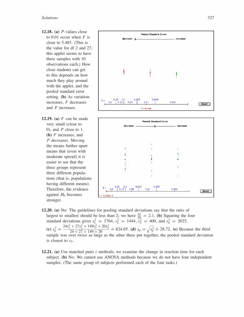
12.18. (a) P-values closeto 0.01 occur when F isclose to 5.483. (This isthe value for df 2 and 27;this applet seems to havethree samples with 10observations each.) Howclose students can getto this depends on howmuch they play aroundwith the applet, and thepooled standard errorsetting. (b) As variationincreases, F decreasesand P increases.

12.19. (a) F can be madevery small (close to0), and P close to 1.(b) F increases, andP decreases. Movingthe means farther apartmeans that (even withmoderate spread) it iseasier to see that thethree groups representthree different popula-tions (that is, populationshaving different means).Therefore, the evidenceagainst H0 becomesstronger.

12.20. (a) No: The guidelines for pooling standard deviations say that the ratio oflargest to smallest should be less than 2; we have 42

20 = 2.1. (b) Squaring the fourstandard deviations gives s2

1 = 1764, s22 = 1444, s2

3 = 400, and s24 = 2025.

(c) s2p = 24s2

1 + 27s22 + 149s2

3 + 20s24

24 + 27 + 149 + 20.= 824.65. (d) sp =

√s2p

.= 28.72. (e) Because the thirdsample was over twice as large as the other three put together, the pooled standard deviationis closest to s3.

12.21. (a) Use matched pairs t methods; we examine the change in reaction time for eachsubject. (b) No: We cannot use ANOVA methods because we do not have four independentsamples. (The same group of subjects performed each of the four tasks.)


12.22. We have x1 = 96.38, s1 = 29.78, n1 = 71, x2 = 109.44, s2 = 31.05, and n2 = 37. Forthe pooled t procedure, we find sp

.= 30.22 and t = −2.13 (df = 106, P.= 0.035). The

Minitab output below shows that F = 4.54 (t2, up to rounding error).

Minitab outputAnalysis of VarianceSource DF SS MS F pFactor 1 4149 4149 4.54 0.035Error 106 96787 913Total 107 100936

12.23. (a) With I = 4 and N = 2290, the degrees of freedom are DFG = I − 1 = 3 andDFE = N − I = 2286. (b) MSE = s2

p = 4.6656, so F = MSGMSE = 11.806

4.6656.= 2.5304. (c) The

F(3, 1000) entry in Table E gives 0.05 < P < 0.10; software give P.= 0.0555.

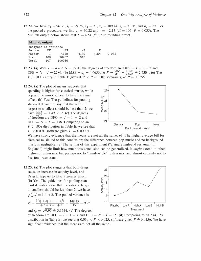
12.24. (a) The plot of means suggests thatspending is higher for classical music, whilepop and no music appear to have the sameeffect. (b) Yes: The guidelines for poolingstandard deviations say that the ratio oflargest to smallest should be less than 2; wehave 3.332

2.243.= 1.49 < 2. (c) The degrees

of freedom are DFG = I − 1 = 2 andDFE = N − I = 138. Comparing to anF(2, 100) distribution in Table E, we see thatP < 0.001; software gives P

.= 0.00005.We have strong evidence that the means are not all the same. (d) The higher average bill forclassical music led to this conclusion; the difference between pop music and no backgroundmusic is negligible. (e) The setting of this experiment (“a single high-end restaurant inEngland”) might limit how much this conclusion can be generalized. It might extend to otherhigh-end restaurants, but perhaps not to “family-style” restaurants, and almost certainly not tofast-food restaurants.

X

XX

Classical Pop None21

22

23

24

Mea

n bi

ll ($

)

Background music

12.25. (a) The plot suggests that both drugscause an increase in activity level, andDrug B appears to have a greater effect.(b) Yes: The guidelines for pooling stan-dard deviations say that the ratio of largestto smallest should be less than 2; we have√

12.256.25 = 1.4 < 2. The pooled variance is

s2p = 3(s2

1 + s22 + · · · + s2

5)

3 + 3 + 3 + 3 + 3= 149.25

15= 9.95

and sp = √9.95 .= 3.1544. (c) The degrees

of freedom are DFG = I − 1 = 4 and DFE = N − I = 15. (d) Comparing to an F(4, 15)

distribution in Table E, we see that 0.010 < P < 0.025; software gives P.= 0.0156. We have

significant evidence that the means are not all the same.

X

X

X

X

X

Placebo Low A High A Low B High B12

14

16

18

20

22

Act

ivity

leve

l

Treatment

Solutions 329

12.26. (a) It is useful to connect the points onthe plot, to make the pattern (or lack thereof)more evident. There is some suggestion thataverage grade decreases as the number ofaccommodations increases. (b) Having toomany decimal points is distracting; in thissituation, no useful information is gainedby having more than one or two digitsafter the decimal point. For example, thefirst mean and standard deviation wouldbe more effectively presented as 2.79 and0.85. (c) The largest-to-smallest SD ratio is slightly over 2 (about 2.009), so pooling is notadvisable. (If we pool in spite of this, we find sp

.= 0.8589.) (d) Eliminating data points(without a legitimate reason) is always risky, although we could run the analysis with andwithout them. Combining the last three groups would be a bad idea if the data suggested thatgrades rebounded after 2 accommodations (i.e., if the average grades were higher for 3 and4 accommodations), but as that is not the case, lumping 2, 3, and 4 accommodations seemsreasonable. (e) ANOVA is not appropriate for these data, chiefly because we do not have 245independent observations. (f) There may be a number of local factors (for example, studentdemographics or teachers’ attitudes toward accommodations) which affected grades; theseeffects might not be the same elsewhere. (g) One weakness is that we do not have a controlgroup for comparison; that is, we cannot tell what grades these students (or a similar group)would have had without accommodations.

0 1 2 3 42.4

2.5

2.6

2.7

2.8

2.9

Mea

n gr

ade

Number of accommodations

12.27. (a) The variation in sample size is some causefor concern, but there can be no extreme outliersin a 1-to-7 scale, so ANOVA is probably reliable.(b) Pooling is reasonable: 1.26

1.03.= 1.22 < 2. (c) With

I = 5 groups and total sample size N = 410, we usean F(4, 405) distribution. We can compare 5.69 to anF(4, 200) distribution in Table E and conclude that P < 0.001, or with software determinethat P

.= 0.0002. (d) Hispanic Americans have the highest emotion scores, Japanese are inthe middle, and the other three cultures are the lowest (and very similar).

60 1 2

5.69

3 4 5


12.28. (a) The largest-to-smallest SD ratios are2.84, 1.23, and 1.14, so the text’s guidelinesare satisfied for intensity and recall, but notfor frequency. (b) As in the previous exercise,I = 5 and N = 410, so we use an F(4, 405)

distribution. From the F(4, 200) distribution inTable E, we can conclude that P < 0.001 forall three response variables. With software, wefind that the P-values are much smaller; all areless than 0.00002. We conclude that, for eachvariable, we have strong evidence that somegroup mean is different. (This conclusion iscautious in the case of frequency because of ourconcern about the standard deviations.) (c) Thetable below shows one way of summarizing themeans. For each variable, it attempts to identifylow (underlined), medium, and high (boldface)values of that variable. Hispanic Americans werehigher than other groups for all four variables.Asian Americans were low for all variables (thelowest in all but global score). Japanese were low on all but global score, while EuropeanAmericans and Indians were in the middle for all but global score. (d) The results might notgeneralize to, for example, subjects who are from different parts of their countries or not in acollege or university community. (e) Create a two-way table with counts of men and womenin each cultural group. The Minitab output on the right gives X2 = 11.353, df = 4, andP = 0.023, so we have evidence (significant at α = 0.05) that the gender mix was not thesame for all cultures. Specifically, Hispanic Americans and European Americans had higherpercentages of women, which might further affect how much we can generalize the results.

Minitab outputWomen Men Total

1 38 8 4631.64 14.36

2 22 11 3322.70 10.30

3 57 34 9162.59 28.41

4 102 58 160110.05 49.95

5 63 17 8055.02 24.98

Total 282 128 410

ChiSq = 1.279 + 2.817 +0.021 + 0.047 +0.499 + 1.100 +0.589 + 1.297 +1.156 + 2.547 = 11.353

df = 4, p = 0.023

Score Frequency Intensity RecallEuropean Amer. 4.39 82.87 2.79 49.12Asian Amer. 4.35 72.68 2.37 39.77Japanese 4.72 73.36 2.53 43.98Indian 4.34 82.71 2.87 49.86Hispanic Amer. 5.04 92.25 3.21 59.99

Solutions 331

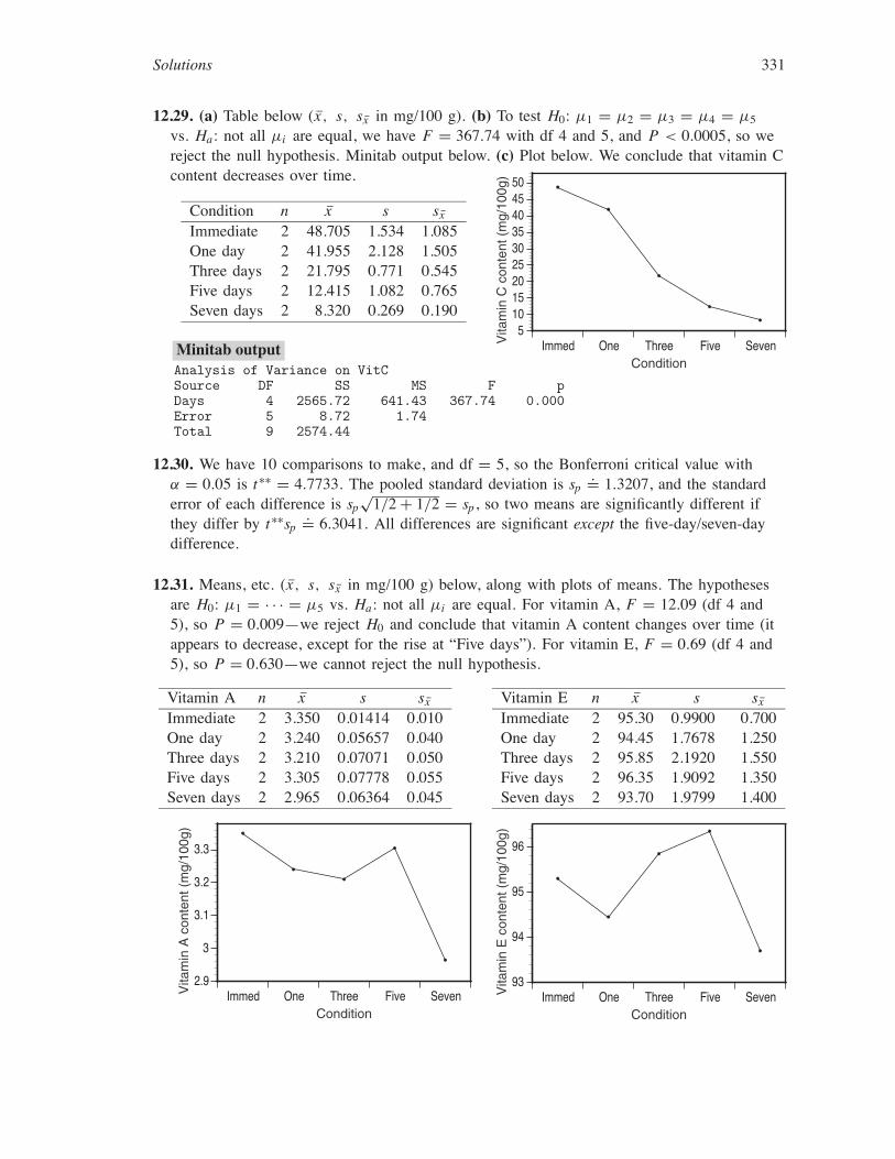
12.29. (a) Table below (x, s, sx in mg/100 g). (b) To test H0: µ1 = µ2 = µ3 = µ4 = µ5

vs. Ha: not all µi are equal, we have F = 367.74 with df 4 and 5, and P < 0.0005, so wereject the null hypothesis. Minitab output below. (c) Plot below. We conclude that vitamin Ccontent decreases over time.

Condition n x s sx

Immediate 2 48.705 1.534 1.085One day 2 41.955 2.128 1.505Three days 2 21.795 0.771 0.545Five days 2 12.415 1.082 0.765Seven days 2 8.320 0.269 0.190

Immed One Three Five Seven5

101520253035404550

Vita

min

C c

onte

nt (

mg/

100g

)

ConditionMinitab outputAnalysis of Variance on VitCSource DF SS MS F pDays 4 2565.72 641.43 367.74 0.000Error 5 8.72 1.74Total 9 2574.44

12.30. We have 10 comparisons to make, and df = 5, so the Bonferroni critical value withα = 0.05 is t∗∗ = 4.7733. The pooled standard deviation is sp

.= 1.3207, and the standarderror of each difference is sp

√1/2 + 1/2 = sp, so two means are significantly different if

they differ by t∗∗sp.= 6.3041. All differences are significant except the five-day/seven-day

difference.

12.31. Means, etc. (x, s, sx in mg/100 g) below, along with plots of means. The hypothesesare H0: µ1 = · · · = µ5 vs. Ha: not all µi are equal. For vitamin A, F = 12.09 (df 4 and5), so P = 0.009—we reject H0 and conclude that vitamin A content changes over time (itappears to decrease, except for the rise at “Five days”). For vitamin E, F = 0.69 (df 4 and5), so P = 0.630—we cannot reject the null hypothesis.

Vitamin A n x s sx


Vitamin E n x s sx


Immed One Three Five Seven2.9

3

3.1

3.2

3.3

Vita

min

A c

onte

nt (

mg/

100g

)

ConditionImmed One Three Five Seven

93

94

95

96

Vita

min

E c

onte

nt (

mg/

100g

)

Condition


Minitab outputAnalysis of Variance on VitASource DF SS MS F pDays 4 0.17894 0.04473 12.09 0.009Error 5 0.01850 0.00370Total 9 0.19744---------------------------------------------------Analysis of Variance on VitESource DF SS MS F pDays 4 9.09 2.27 0.69 0.630Error 5 16.47 3.29Total 9 25.56

12.32. (a) We did not reject H0 for vitamin E, so we have no reason to believe that any meansare different. (b) As in Exercise 12.30, t∗∗ = 4.7733. The pooled standard deviation issp

.= 0.06083 and the standard error of each difference is sp√

1/2 + 1/2 = sp, so twomeans are significantly different if they differ by t∗∗sp

.= 0.2903. By this standard, only theimmediate/seven-day and five-day/seven-day differences are significant.

12.33. There is no significant evidence of change in vitamin E content. Vitamin C contentdecreases over time, with significant change occurring over the first five days. Forvitamin A, the fluctuations over the first five days are not significant, but the drop fromday 5 to day 7 is.

12.34. (a) Means, standard deviations, and standard errors of the mean are below, along witha plot of the means. Note that the standard deviations grossly violate our guideline forpooling: 1066.97

89.94.= 11.86. As we might expect, spores are highest in the summer, and lowest

in the winter. (b) ANOVA gives F = 4.83 (df 3 and 8) and P = 0.033—the differences aresignificant at the 5% level. (The small samples and large variation make the seemingly largedifferences not as significant as we might expect.)

n x s sx

Fall 3 1191 89.94 51.926Winter 3 195 163.72 94.522Spring 3 1216 773.12 446.360Summer 3 2263.6 1066.97 616.014

Fall Winter Spring Summer0

500

1000

1500

2000

Mea

n sp

ores

(C

FU

/m3 a

ir)

SeasonMinitab outputAnalysis of VarianceSource DF SS MS F pFactor 3 6422013 2140671 4.83 0.033Error 8 3542047 442756Total 11 9964060

Solutions 333

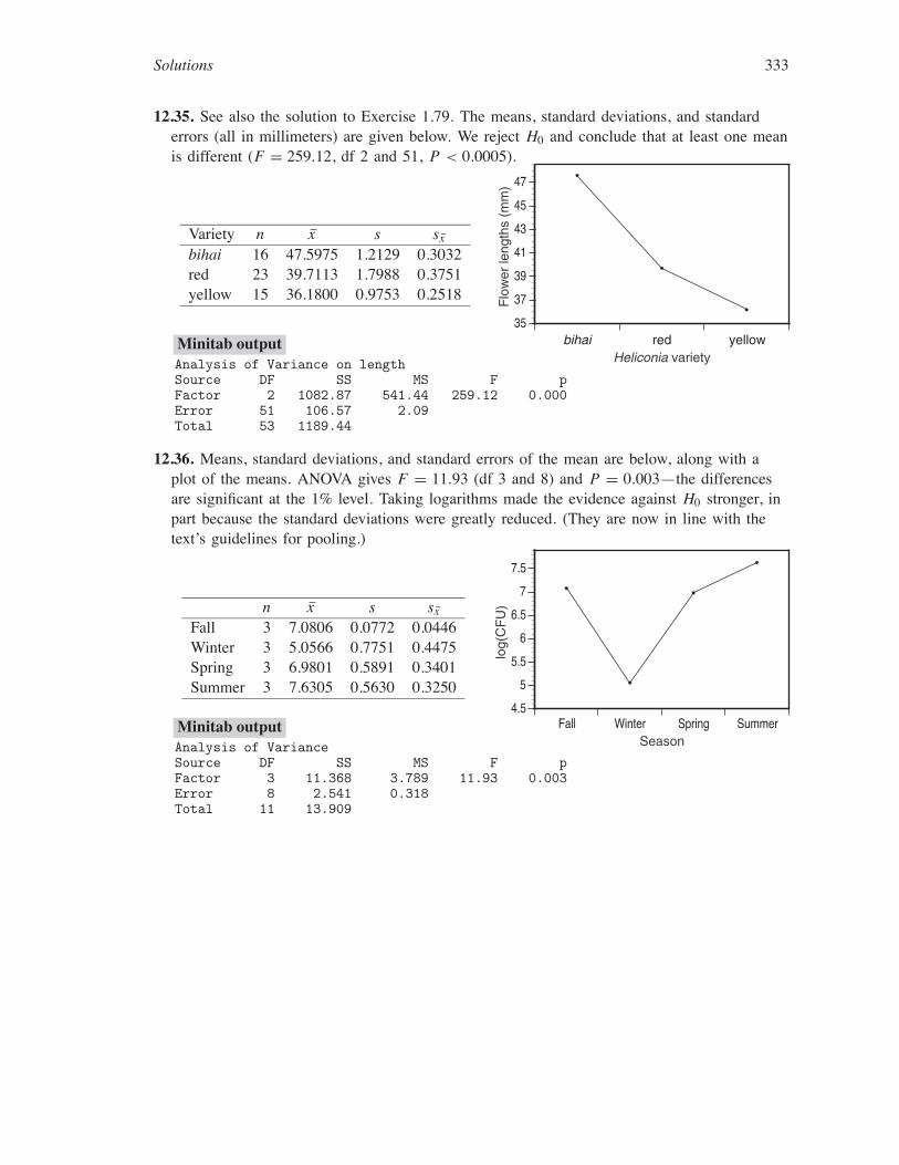
12.35. See also the solution to Exercise 1.79. The means, standard deviations, and standarderrors (all in millimeters) are given below. We reject H0 and conclude that at least one meanis different (F = 259.12, df 2 and 51, P < 0.0005).

Variety n x s sx

bihai 16 47.5975 1.2129 0.3032red 23 39.7113 1.7988 0.3751yellow 15 36.1800 0.9753 0.2518

bihai red yellow35

37

39

41

43

45

47

Flo

wer

leng

ths

(mm

)

Heliconia varietyMinitab outputAnalysis of Variance on lengthSource DF SS MS F pFactor 2 1082.87 541.44 259.12 0.000Error 51 106.57 2.09Total 53 1189.44

12.36. Means, standard deviations, and standard errors of the mean are below, along with aplot of the means. ANOVA gives F = 11.93 (df 3 and 8) and P = 0.003—the differencesare significant at the 1% level. Taking logarithms made the evidence against H0 stronger, inpart because the standard deviations were greatly reduced. (They are now in line with thetext’s guidelines for pooling.)

n x s sx

Fall 3 7.0806 0.0772 0.0446Winter 3 5.0566 0.7751 0.4475Spring 3 6.9801 0.5891 0.3401Summer 3 7.6305 0.5630 0.3250

Fall Winter Spring Summer4.5

5

5.5

6

6.5

7

7.5

log(

CF

U)

SeasonMinitab outputAnalysis of VarianceSource DF SS MS F pFactor 3 11.368 3.789 11.93 0.003Error 8 2.541 0.318Total 11 13.909


12.37. The means, standard deviations, and standard errors are given below. We reject H0 andconclude that at least one mean is different (F = 244.27, df 2 and 51, P < 0.0005). Theseresults are essentially the same as in Exercise 12.35.

Variety n x s sx

bihai 16 3.8625 0.02515 0.006286red 23 3.6807 0.04496 0.009374yellow 15 3.5882 0.02698 0.006966

bihai red yellow3.55

3.6

3.65

3.7

3.75

3.8

3.85

log(

Flo

wer

leng

ths)

Heliconia varietyMinitab outputAnalysis of Variance on loglenSource DF SS MS F pFactor 2 0.61438 0.30719 244.27 0.000Error 51 0.06414 0.00126Total 53 0.67852

12.38. (a) Statistics and plots are below. (b) The standard deviations satisfy the text’sguidelines for pooling. One concern is that all three distributions are slightly left-skewed andthe youngest nonfiction death is an outlier. (c) ANOVA gives F = 6.56 (df 2 and 120) andP = 0.002, so we conclude that at least one mean is different. (d) The appropriate contrastis ψ1 = 1

2(µnov + µnf) − µp. (This is defined so that the ψ1 > 0 if poets die younger. Thisis not absolutely necessary but is in keeping with the text’s advice.) The null hypothesis isH0: ψ1 = 0; the Yeats quote hardly seems like an adequate reason to choose a one-sidedalternative, but students may have other opinions. For the test, we compute c

.= 10.9739,SEc

.= 3.0808, and t.= 3.56 with df = 120. The P-value is very small regardless of whether

Ha is one- or two-sided, so we conclude that the contrast is positive (and poets die young).(e) For this comparison, the contrast is ψ2 = µnov − µnf, and the hypotheses are H0: ψ2 = 0vs. Ha: ψ2 �= 0. (Because the alternative is two-sided, the subtraction in this contrast can goeither way.) For the test, we compute c

.= −5.4272, SEc.= 3.4397, and t

.= −1.58 withdf = 120. This gives P = 0.1172; the difference between novelists and nonfiction writers isnot significant. (f) With three comparisons and df = 120, the Bonferroni critical value ist∗∗ = 2.4280. The pooled standard deviation is sp

.= 14.4592, so the differences, standarderrors, and t values are:

xnov − xp.= 8.2603, SEnov−p = sp

√167 + 1

32.= 3.1071, t

.= 2.66

xnov − xnf.= −5.4272, SEnov−nf = sp

√1

67 + 124

.= 3.4397, t.= −1.58

xp − xnf.= −13.6875, SEp−nf = sp

√132 + 1

24.= 3.9044, t

.= −3.51

The first and last differences are greater (in absolute value) than t∗∗, so those differencesare significant. The second difference is the same one tested in the contrast of part (e); thestandard error and the conclusion are the same.

Solutions 335

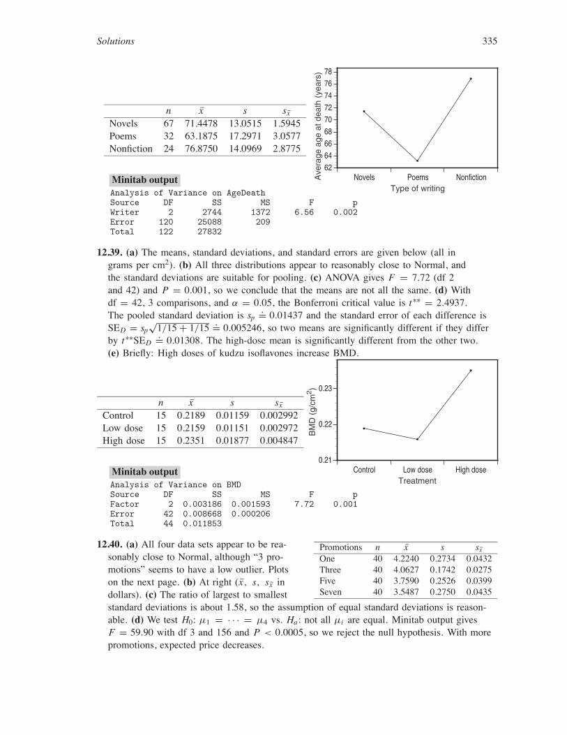
n x s sx

Novels 67 71.4478 13.0515 1.5945Poems 32 63.1875 17.2971 3.0577Nonfiction 24 76.8750 14.0969 2.8775

Novels Poems Nonfiction626466687072747678

Ave

rage

age

at d

eath

(ye

ars)

Type of writingMinitab outputAnalysis of Variance on AgeDeathSource DF SS MS F pWriter 2 2744 1372 6.56 0.002Error 120 25088 209Total 122 27832

12.39. (a) The means, standard deviations, and standard errors are given below (all ingrams per cm2). (b) All three distributions appear to reasonably close to Normal, andthe standard deviations are suitable for pooling. (c) ANOVA gives F = 7.72 (df 2and 42) and P = 0.001, so we conclude that the means are not all the same. (d) Withdf = 42, 3 comparisons, and α = 0.05, the Bonferroni critical value is t∗∗ = 2.4937.The pooled standard deviation is sp

.= 0.01437 and the standard error of each difference isSED = sp

√1/15 + 1/15 .= 0.005246, so two means are significantly different if they differ

by t∗∗SED.= 0.01308. The high-dose mean is significantly different from the other two.

(e) Briefly: High doses of kudzu isoflavones increase BMD.

n x s sx

Control 15 0.2189 0.01159 0.002992Low dose 15 0.2159 0.01151 0.002972High dose 15 0.2351 0.01877 0.004847

Control Low dose High dose0.21

0.22

0.23

BM

D (

g/cm

2 )

TreatmentMinitab outputAnalysis of Variance on BMDSource DF SS MS F pFactor 2 0.003186 0.001593 7.72 0.001Error 42 0.008668 0.000206Total 44 0.011853

12.40. (a) All four data sets appear to be rea-sonably close to Normal, although “3 pro-motions” seems to have a low outlier. Plotson the next page. (b) At right (x, s, sx indollars). (c) The ratio of largest to smalleststandard deviations is about 1.58, so the assumption of equal standard deviations is reason-able. (d) We test H0: µ1 = · · · = µ4 vs. Ha: not all µi are equal. Minitab output givesF = 59.90 with df 3 and 156 and P < 0.0005, so we reject the null hypothesis. With morepromotions, expected price decreases.

Promotions n x s sx

One 40 4.2240 0.2734 0.0432Three 40 4.0627 0.1742 0.0275Five 40 3.7590 0.2526 0.0399Seven 40 3.5487 0.2750 0.0435


One Promotion

3.50

3.75

4.00

4.25

4.50

4.75

–3 –2 –1 0 1 2 3

Exp

ecte

d pr

ice

z score

Three Promotions

3.50

3.75

4.00

4.25

–3 –2 –1 0 1 2 3

Exp

ecte

d pr

ice

z score

Five Promotions

3.25

3.50

3.75

4.00

4.25

–3 –2 –1 0 1 2 3

Exp

ecte

d pr

ice

z score

Seven Promotions

2.75

3.00

3.25

3.50

3.75

4.00

–3 –2 –1 0 1 2 3

Exp

ecte

d pr

ice

z score

Minitab outputAnalysis of Variance on ExpPriceSource DF SS MS F pNumPromo 3 10.9885 3.6628 59.90 0.000Error 156 9.5388 0.0611Total 159 20.5273

12.41. We have six comparisons to make, and df = 156, so the Bonferroni critical valuewith α = 0.05 is t∗∗ = 2.6723. The pooled standard deviation is sp

.= 0.2473, so thestandard error of each difference is SED = sp

√1/40 + 1/40 .= 0.05529. Two means must

differ by t∗∗SED.= 0.1477 in order to be significantly different; all six differences are

significant. (Note that because the means decrease, we could consider only the differences inconsecutive means, that is, x1 − x3, x3 − x5, and x5 − x7. Since these three differences aresignificant, it follows that the others must be, too.)

x1 − x3 = 0.16125 t13 = 2.916x1 − x5 = 0.46500 t15 = 8.410x1 − x7 = 0.67525 t17 = 12.212x3 − x5 = 0.30375 t35 = 5.493x3 − x7 = 0.51400 t37 = 9.296x5 − x7 = 0.21025 t57 = 3.802

One Three Five Seven3.50

3.75

4.00

4.25

Exp

ecte

d pr

ice

Promotions

Solutions 337

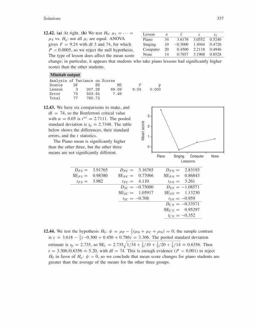
12.42. (a) At right. (b) We test H0: µ1 = · · · =µ4 vs. Ha: not all µi are equal. ANOVAgives F = 9.24 with df 3 and 74, for whichP < 0.0005, so we reject the null hypothesis.The type of lesson does affect the mean scorechange; in particular, it appears that students who take piano lessons had significantly higherscores than the other students.

Lesson n x s sx

Piano 34 3.6176 3.0552 0.5240Singing 10 −0.3000 1.4944 0.4726Computer 20 0.4500 2.2118 0.4946None 14 0.7857 3.1908 0.8528

Minitab outputAnalysis of Variance on ScoresSource DF SS MS F pLesson 3 207.28 69.09 9.24 0.000Error 74 553.44 7.48Total 77 760.72

12.43. We have six comparisons to make, anddf = 74, so the Bonferroni critical valuewith α = 0.05 is t∗∗ = 2.7111. The pooledstandard deviation is sp

.= 2.7348. The tablebelow shows the differences, their standarderrors, and the t statistics.

The Piano mean is significantly higherthan the other three, but the other threemeans are not significantly different.

Piano Singing Computer None

0

1

2

3

Mea

n sc

ore

Lessons

DP S = 3.91765SEP S = 0.98380

tP S = 3.982

DPC = 3.16765SEPC = 0.77066

tPC = 4.110

DP N = 2.83193SEP N = 0.86843

tP N = 3.261DSC = −0.75000

SESC = 1.05917tSC = −0.708

DSN = −1.08571SESN = 1.13230

tSN = −0.959DC N = −0.33571

SEC N = 0.95297tC N = −0.352

12.44. We test the hypothesis H0: ψ = µP − 13(µS + µC + µN) = 0; the sample contrast

is c.= 3.618 − 1

3(−0.300 + 0.450 + 0.786) = 3.306. The pooled standard deviation

estimate is sp = 2.735, so SEc = 2.735√

1/34 + 19/10 + 1

9/20 + 19/14 .= 0.6356. Then

t = 3.306/0.6356 .= 5.20, with df = 74. This is enough evidence (P < 0.001) to rejectH0 in favor of Ha: ψ > 0, so we conclude that mean score changes for piano students aregreater than the average of the means for the other three groups.


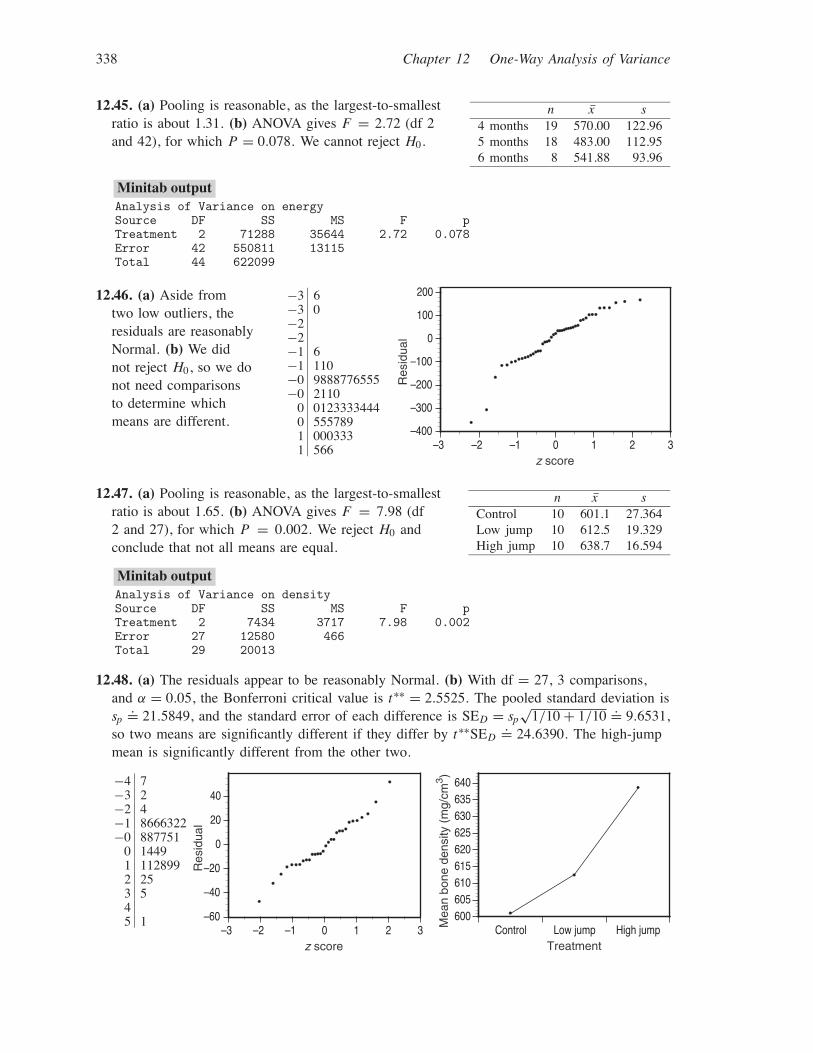
12.45. (a) Pooling is reasonable, as the largest-to-smallestratio is about 1.31. (b) ANOVA gives F = 2.72 (df 2and 42), for which P = 0.078. We cannot reject H0.

n x s4 months 19 570.00 122.965 months 18 483.00 112.956 months 8 541.88 93.96

Minitab outputAnalysis of Variance on energySource DF SS MS F pTreatment 2 71288 35644 2.72 0.078Error 42 550811 13115Total 44 622099

12.46. (a) Aside fromtwo low outliers, theresiduals are reasonablyNormal. (b) We didnot reject H0, so we donot need comparisonsto determine whichmeans are different.

−3 6−3 0−2−2−1 6−1 110−0 9888776555−0 2110

0 01233334440 5557891 0003331 566

–400

–300

–200

–100

0

100

200

–3 –2 –1 0 1 2 3

Res

idua

l

z score

12.47. (a) Pooling is reasonable, as the largest-to-smallestratio is about 1.65. (b) ANOVA gives F = 7.98 (df2 and 27), for which P = 0.002. We reject H0 andconclude that not all means are equal.

n x sControl 10 601.1 27.364Low jump 10 612.5 19.329High jump 10 638.7 16.594

Minitab outputAnalysis of Variance on densitySource DF SS MS F pTreatment 2 7434 3717 7.98 0.002Error 27 12580 466Total 29 20013

12.48. (a) The residuals appear to be reasonably Normal. (b) With df = 27, 3 comparisons,and α = 0.05, the Bonferroni critical value is t∗∗ = 2.5525. The pooled standard deviation issp

.= 21.5849, and the standard error of each difference is SED = sp√

1/10 + 1/10 .= 9.6531,so two means are significantly different if they differ by t∗∗SED

.= 24.6390. The high-jumpmean is significantly different from the other two.

−4 7−3 2−2 4−1 8666322−0 887751

0 14491 1128992 253 545 1 –60

–40

–20

0

20

40

–3 –2 –1 0 1 2 3

Res

idua

l

z scoreControl Low jump High jump

600605610615620625630635640

Mea

n bo

ne d

ensi

ty (

mg/

cm3 )

Treatment

Solutions 339

12.49. (a) Pooling is risky because 0.6283/0.2520 =2.49 > 2. (b) ANOVA gives F = 31.16 (df 2 and 9),for which P < 0.0005. We reject H0 and conclude thatnot all means are equal.

n x sAluminum 4 2.0575 0.2520Clay 4 2.1775 0.6213Iron 4 4.6800 0.6283

Minitab outputAnalysis of Variance on ironSource DF SS MS F pPot 2 17.539 8.770 31.16 0.000Error 9 2.533 0.281Total 11 20.072

12.50. (a) There are no clear violations of Normality, but the number of residuals is so smallthat is difficult to draw any conclusions. (b) With df = 9, 3 comparisons, and α = 0.05,the Bonferroni critical value is t∗∗ = 2.9333. The pooled standard deviation is sp

.= 0.5305,and the standard error of each difference is SED = sp

√1/4 + 1/4 .= 0.3751, so two means

are significantly different if they differ by t∗∗SED.= 1.1003. The iron mean is significantly

higher than the other two.

−0 8−0 6−0 4−0 2−0 0

0 000 330 455

–1–0.8–0.6–0.4–0.2

00.20.40.6

–2 –1 0 1 2

Res

idua

l

z scoreAluminum Clay Iron

1.5

2

2.5

3

3.5

4

4.5

Mea

n iro

n (m

g/10

0g)

Pot type

12.51. (a) Pooling is risky because 8.66/2.89 = 3 > 2.(b) ANOVA gives F = 137.94 (df 5 and 12), for whichP < 0.0005. We reject H0 and conclude that not allmeans are equal.

n x sECM1 3 65.0% 8.6603%ECM2 3 63.3% 2.8868%ECM3 3 73.3% 2.8868%MAT1 3 23.3% 2.8868%MAT2 3 6.6% 2.8868%MAT3 3 11.6% 2.8868%

Minitab outputAnalysis of Variance on gpiSource DF SS MS F pTreatment 5 13411.1 2682.2 137.94 0.000Error 12 233.3 19.4Total 17 13644.4

12.52. (a) The residuals have one low outlier, and a lot of granularity, so Normality isdifficult to assess. (b) With df = 12, 15 comparisons, and α = 0.05, the Bonferronicritical value is t∗∗ = 3.6489. The pooled standard deviation is sp

.= 4.4096%, andthe standard error of each difference is SED = sp

√1/3 + 1/3 .= 3.6004%, so two

means are significantly different if they differ by t∗∗SED.= 13.1375%. The three

ECM means are significantly higher than the three MAT means. (c) The contrast isψ = 1

3(µECM1 + µECM2 + µECM3) − 13(µMAT1 + µMAT2 + µMAT3), and the hypotheses are

H0: ψ = 0 vs. Ha: ψ �= 0. For the test, we compute c.= 53.33%, SEc

.= 2.0787%, and


t.= 25.66 with df = 12. This has a tiny P-value; the difference between ECM and MAT is

highly significant. This is consistent with the Bonferroni results from part (b).

−1 0−0−0−0−0 333−0 1111

0 1111110 330 55

–12–10–8–6–4–2

0246

–3 –2 –1 0 1 2 3

Res

idua

l

z scoreECM1 ECM2 ECM3 MAT1 MAT2 MAT3

0

10

20

30

40

50

60

70

Mea

n %

Gpi

cel

ls

Pot type

12.53. Let µ1 be the placebo mean, µ2 and µ3 be the means for low and high dosesof Drug A, and µ4 and µ5 be the means for low and high doses of Drug B.Recall that sp

.= 3.1544. (a) The first contrast is ψ1 = µ1 − 0.5µ2 − 0.5µ4;the second is ψ2 = µ3 − µ2 − (µ5 − µ4). (b) The estimated contrasts are c1 =14.00 − 0.5(15.25) − 0.5(16.75) = −2 and c2 = (18.25 − 15.25) − (22.50 − 16.75) = −2.75.The respective standard errors are:

SEc1 = sp

√14

+ 0.254

+ 04

+ 0.254

+ 04

.= 1.9316 and

SEc2 = sp

√04

+ 14

+ 14

+ 14

+ 14

.= 3.1544

(c) Neither contrast is significant (t1.= −1.035 and t2

.= −0.872, for which the P-valuesare 0.1584 and 0.1985). We do not have enough evidence to conclude that low dosesincrease activity level over a placebo, nor can we conclude that activity level changes due toincreased dosage are different between the two drugs.

12.54. (a) Below. (b) To test H0: µ1 = · · · = µ4 vs. Ha: not all µi are equal, ANOVA(Minitab output below) gives F = 967.82 (df 3 and 351), which has P < 0.0005. Weconclude that not all means are equal; specifically, the “Placebo” mean is much higher thanthe other three means.

Shampoo n x s sx

PyrI 112 17.393 1.142 0.108PyrII 109 17.202 1.352 0.130Keto 106 16.028 0.931 0.090Placebo 28 29.393 1.595 0.301

PyrI PyrII Keto Placebo15

20

25

30

Mea

n sc

alp

flaki

ng r

atin

g

ShampooMinitab outputAnalysis of Variance on FlakingSource DF SS MS F pCode 3 4151.43 1383.81 967.82 0.000Error 351 501.87 1.43Total 354 4653.30

Solutions 341

12.55. (a) The plot (below) shows granularity (which varies between groups), but that shouldnot make us question independence; it is due to the fact that the scores are all integers.(b) The ratio of the largest to the smallest standard deviations is 1.595/0.931 .= 1.714—lessthan 2. (c) Apart from the granularity, the quantile plots (below) are reasonably straight.(d) Again, apart from the granularity, the quantile plot looks pretty good.

12.55(a)

–4

–3

–2

–1

0

1

2

3

4

0 50 100 150 200 250 300 350

Res

idua

l

Case

12.55(d)

–4

–3

–2

–1

0

1

2

3

4

–3 –2 –1 0 1 2 3

Res

idua

l

z score

12.55(c)–PyrI

14

15

16

17

18

19

20

–3 –2 –1 0 1 2 3

Pyr

I fla

king

sco

re

z score

12.55(c)–PyrII

131415161718192021

–3 –2 –1 0 1 2 3

Pyr

II fla

king

sco

re

z score

12.55(c)–Keto

13

14

15

16

17

18

–3 –2 –1 0 1 2 3

Ket

o fla

king

sco

re

z score

12.55(c)–Placebo

25

26

27

28

29

30

31

32

–3 –2 –1 0 1 2 3

Pla

cebo

flak

ing

scor

e

z score


12.56. We have six comparisons to make, and df = 351, so the Bonferroni critical value withα = 0.05 is t∗∗ = 2.6533. The pooled standard deviation is sp = √

MSE .= 1.1958; thedifferences, standard errors, and t statistics are below. The only nonsignificant difference isbetween the two Pyr treatments (meaning the second application of the shampoo is of littlebenefit). The Keto shampoo mean is the lowest; the placebo mean is by far the highest.

DPy1−Py2 = 0.19102SEPy1−Py2 = 0.16088

tPy1−Py2 = 1.187

DPy1−K = 1.36456SEPy1−K = 0.16203

tPy1−K = 8.421

DPy1−P = −12.0000SEPy1−P = 0.25265

tPy1−P = −47.497DPy2−K = 1.17353

SEPy2−K = 0.16312tPy2−K = 7.195

DPy2−P = −12.1910SEPy2−P = 0.25334

tPy2−P = −48.121DK−P = −13.3646

SEK−P = 0.25407tK−P = −52.601

12.57. (a) The three contrasts are:

ψ1 = 13µPy1 + 1

3µPy2 + 13µK − µP

ψ2 = 12µPy1 + 1

2µPy2 − µK

ψ3 = µPy1 − µPy2

(b) The pooled standard deviation is sp = √MSE .= 1.1958. The estimated contrasts and

their standard errors are in the table. For example:

SEc1 = sp

√19/112 + 1

9/109 + 19/106 + 1/28 .= 0.2355

(c) We test H0: ψi = 0 vs. Ha: ψi �= 0 for each contrast. The t- and P-values are given inthe table.

The Placebo mean is significantly higher than the average of the other three, while theKeto mean is significantly lower than the average of the two Pyr means. The differencebetween the Pyr means is not significant (meaning the second application of the shampoo isof little benefit)—this agrees with our conclusion from Exercise 12.56.

c1 = −12.51 c2 = 1.269 c3 = 0.191SEc1

.= 0.2355 SEc2

.= 0.1413 SEc3

.= 0.1609t1 = −53.17 t2 = 8.98 t3 = 1.19P1 < 0.0005 P2 < 0.0005 P3

.= 0.2359

12.58. (a) At right. (b) Each new value(except for n) is simply:

(old value)/64 × 100%

(c) The SS and MS entries differ fromthose of Exercise 12.29—by a factor of(100/64)2. However, everything else isthe same: F = 367.74 with df 4 and 5; P < 0.0005, so we (again) reject H0 and concludethat vitamin C content decreases over time.

Condition n x s sx

Immediate 2 76.102% 2.3975% 1.6953%One day 2 65.555% 3.3256% 2.3516%Three days 2 34.055% 1.2043% 0.8516%Five days 2 19.398% 1.6904% 1.1953%Seven days 2 13.000% 0.4198% 0.2969%

Minitab outputAnalysis of Variance on VitCPctSource DF SS MS F pDays 4 6263.97 1565.99 367.74 0.000Error 5 21.29 4.26Total 9 6285.26

Solutions 343

12.59. Transformed values for vitamin A are atright; each value is:

(old value)/5 × 100%

(or equivalently, multiply by 20%). The trans-formation has no effect on vitamin E since thenumber of milligrams remaining is also the percentage of the original 100 mg.

For vitamin A, the SS and MS entries differ from those of Exercise 12.31—by a factor of(100/5)2 = 400. Everything else is the same: F = 12.09 with df 4 and 5; P = 0.009, so we(again) reject H0 and conclude that vitamin A content decreases over time.

Since the vitamin E numbers are unchanged, the ANOVA table is unchanged, and weagain fail to reject H0 (F = 0.69 with df 4 and 5; P = 0.630).

In summary, transforming to percents (or doing any linear transformation) has no effect onthe results of the ANOVA.

Condition n x s sx

Immediate 2 67.0% 0.2828% 0.2%One day 2 64.8% 1.1314% 0.8%Three days 2 64.2% 1.4142% 1.0%Five days 2 66.1% 1.5556% 1.1%Seven days 2 59.3% 1.2728% 0.9%

Minitab outputAnalysis of Variance on VitAPctSource DF SS MS F pDays 4 71.58 17.89 12.09 0.009Error 5 7.40 1.48Total 9 78.98

12.60. There is no effect on the test statistic, df, P-value, and conclusion. The degrees offreedom are not affected, since the number of groups and sample sizes are unchanged;meanwhile, the SS and MS values change (by a factor of b2), but this change does notaffect F since the factors of b2 cancel out in the ratio F = MSG/MSE. With the same F-and df values, the P-value and conclusion are necessarily unchanged.

Proof of these statements is not too difficult, but it requires careful use of the SSformulas. For most students, a demonstration with several choices of a and b wouldprobably be more convincing than a proof. However, here is the basic idea: Using resultsof Chapter 1, we know that the means undergo the same transformation as the data(x∗

i = a + bxi ), while the standard deviations are changed by a factor of |b|. Let x be theaverage of all the data; note that x∗ = a + bx . Now SSG = ∑I

i=1 ni (xi − x)2, so:

SSG∗ = ∑i ni (x∗

i − x∗)2 = ∑i ni (b xi − b x)2 = ∑

i ni b2(xi − x)2 = b2SSG

Similarly, we can establish that SSE∗ = b2SSE and SST∗ = b2SST. Since the MS values aremerely SS values divided by the (unchanged) degrees of freedom, these also change by afactor of b2.

12.61. A table of means and standard deviations is given on the next page. Quantile plots arenot shown, but apart from the granularity of the scores and a few possible outliers, there areno marked deviations from Normality. Pooling is reasonable for both PRE1 and PRE2; theratios are 1.24 and 1.48.

For both PRE1 and PRE2, we test H0: µB = µD = µS vs. Ha: at least one mean isdifferent. Both tests have df 2 and 63. For PRE1, F = 1.13 and P = 0.329; for PRE2,F = 0.11 and P = 0.895. There is no reason to believe that the mean pretest scores differbetween methods.


PRE1 PRE2Method n x s x s

Basal 22 10.5 2.9721 5.27 2.7634DRTA 22 9.72 2.6936 5.09 1.9978Strat 22 9.136 3.3423 4.954 1.8639

Minitab outputAnalysis of Variance on pre1Source DF SS MS F pGroup 2 20.58 10.29 1.13 0.329Error 63 572.45 9.09Total 65 593.03

Analysis of Variance on pre2Source DF SS MS F pGroup 2 1.12 0.56 0.11 0.895Error 63 317.14 5.03Total 65 318.26

12.62. Some of the distributions have mild outliersor skewness, but there are no serious violations ofNormality evident. Pooling is appropriate for allthree response variables.

The three F statistics, all with df 2 and 63, are 5.32 (P = 0.007), 8.41 (P = 0.001), and4.48 (P = 0.015). We conclude that at least one mean is different for each posttest.

For multiple comparisons, we have three comparisons, df 63, and α = 0.05, so theBonferroni critical value is t∗∗ = 2.4596. In the table on the right are the pooled standarddeviations, standard error of each difference, and values of t∗∗SED (the “minimum significantdifference,” or MSD) for each response variable. For both POST1 and POST3, DRTA issignificantly greater than Basal, but no other comparisons are significant. For POST2, Strat issignificantly greater than both Basal and DRTA.

We also may examine the contrasts ψ1 = −µB + 12(µD + µS), which is positive if the

average of the new methods is greater than the basal mean, and ψ2 = µD − µS, whichcompares the two new methods. Estimated contrasts, standard errors, t , and P are given inthe table below. (The P-values are one-sided for ψ1 and two-sided for ψ2.) We see that c1 issignificantly positive for all three variables. The second contrast was included in our multiplecomparisons, where we found the difference significant only for POST2, but this time, whenwe are testing only this difference, rather than all three possible differences, we conclude thatµD > µS for POST1, in addition to the difference for POST2.

Variable sp SED t∗∗SED

POST1 3.1885 0.9614 2.3646POST2 2.3785 0.7171 1.7639POST3 6.3141 1.9038 4.6825

Variable c1 SEc1 t1 P1 c2 SEc2 t2 P2

POST1 2.0909 0.8326 2.51 0.0073 2.0000 0.9614 2.08 0.0415POST2 1.7500 0.6211 2.82 0.0032 −2.1364 0.7171 −2.98 0.0041POST3 4.4545 1.6487 2.70 0.0044 2.4545 1.9038 1.29 0.2019

Solutions 345

Basal DRTA Strat6.5

7

7.5

8

8.5

9

9.5

10

Mea

n P

OS

T1

scor

e

Teaching methodBasal DRTA Strat

5

5.5

6

6.5

7

7.5

8

8.5

Mea

n P

OS

T2

scor

e

Teaching methodBasal DRTA Strat

40

41

42

43

44

45

46

47

Mea

n P

OS

T3

scor

e

Teaching method

Test Method x sPOST1 Basal 6.6818 2.7669

DRTA 9.7727 2.7243Strat 7.7727 3.9271

POST2 Basal 5.5455 2.0407DRTA 6.2273 2.0915Strat 8.3636 2.9040

POST3 Basal 41.0455 5.6356DRTA 46.7273 7.3884Strat 44.2727 5.7668

Basal/POST1

12 03 04 0005 000006 07 008 0009 000

10 01112 00

DRTA/POST1

12345 0067 0008 00009

10 000011 0012 00013 0014 00

Strat/POST1

1 023 04 00005 006 07 0008 09 00

1011 0012 0013 014 015 0

Basal/POST2

0123 0004 000005 0000006 07 008 0009 0

10 0

DRTA/POST2

0 0123 045 006 00000000007 00008 009 0

1011 0

Strat/POST2

01 0234 05 006 07 008 0009 0000

10 00011 0012 0013 0

Basal/POST3

33 2233 53 663 994 00114 234 45554 664 9555 4

DRTA/POST3

3 01333 734 014 2344 74 88899995 05 335 4555 7

Strat/POST3

33 333 433 84 14 22234 4554 74 8889995 015 3


Minitab outputAnalysis of Variance on POST1Source DF SS MS F pMethod 2 108.1 54.1 5.32 0.007Error 63 640.5 10.2Total 65 748.6

Analysis of Variance on POST2Source DF SS MS F pMethod 2 95.12 47.56 8.41 0.001Error 63 356.41 5.66Total 65 451.53

Analysis of Variance on POST3Source DF SS MS F pMethod 2 357.3 178.7 4.48 0.015Error 63 2511.7 39.9Total 65 2869.0

12.63. The regression equation is:

y = 4.3645 − 0.1165x

(y is the expected price and x is the numberof promotions). The regression is significant(i.e., the slope is significantly different from0): t = −13.31 with df = 158, givingP < 0.0005. The regression on numberof promotions explains r2 = 52.9% of thevariation in expected price. (This is similarto the ANOVA value: R2 = 53.5%.)

The granularity of the “Number of promotions” observations makes interpreting the resid-ual plot a bit tricky. For five promotions, the residuals seem to be more likely to be nega-tive (in fact, 26 of the 40 residuals are negative), while for 3 promotions, the residuals areweighted toward the positive side. (We also observe that in the plot of mean expected pricevs. number of promotions—see the solution to Exercise 12.40—the mean for 3 promotions isnot as small as one would predict from a line near the other three points.) This suggests thata linear model may not be appropriate.

–0.8

–0.6

–0.4

–0.2

0

0.2

0.4

0.6

1 3 5 7

Res

idua

l

Number of promotions

Minitab outputThe regression equation is ExpPrice = 4.36 - 0.116 NumPromo

Predictor Coef Stdev t-ratio pConstant 4.36452 0.04009 108.87 0.000NumPromo -0.116475 0.008748 -13.31 0.000

s = 0.2474 R-sq = 52.9% R-sq(adj) = 52.6%

Analysis of Variance

SOURCE DF SS MS F pRegression 1 10.853 10.853 177.26 0.000Error 158 9.674 0.061Total 159 20.527

Solutions 347

12.64. The pooled standard deviation sp is found by looking at the spread of each observationabout its group mean xi . The “total” standard deviation s given in Exercise 12.26 is thespread about the grand mean (the mean of all the data values, ignoring distinctions betweengroups). When we ignore group differences, we have more variation (uncertainty) in ourdata, so s is almost always larger than sp.

This can be made clearer (to sufficiently mathematical students) by noting that

the total variance s2 can be found in the ANOVA table: Just as s2p = SSE

DFE= MSE,

s2 = SSTDFT

= MST. (The total mean square is not included in the ANOVA table but is easilycomputed from the values on the bottom line.) Because SSM + SSE = SST, we always haveSSE ≤ SST, with equality only when the model is completely worthless (that is, when allgroup means equal the grand mean). Because DFE < DFT, it might be that MSE ≥ MSTbut that does not happen very often.

12.66. With σ = 7 and means µ1 = 40, µ2 = 47, and µ3 = 43, we have µ = 40+47+433 = 43.3

and noncentrality parameter:

λ = n∑

(µi − µ)2

σ 2 = (10)[(40 − 43.3)2 + (47 − 43.3)2 + (43 − 43.3)2

]49

= (10)(24.6)

49.= 5.0340

(The value of λ in the G•Power output below is slightly different due to rounding.) Thedegrees of freedom and critical value are the same as in Example 12.27: df 2 and 27,F∗ = 3.35. Software reports the power as about 46%. Samples of size 10 are not adequatefor this alternative; we should increase the sample size so that we have a better chance ofdetecting it. (For example, samples of size 20 give nearly 80% power for this alternative.)

G•Power outputPost-hoc analysis for "F-Test (ANOVA)", Global, Groups: 3:Alpha: 0.0500Power (1-beta): 0.4606Effect size "f": 0.4096Total sample size: 30Critical value: F(2,27) = 3.3541Lambda: 5.0332

12.67. (a) Sampling plans will vary but should attempt to address how cultural groups will bedetermined: Can we obtain such demographic information from the school administration?Do we simply select a large sample then poll each student to determine if he or she belongsto one of these groups? (b) Answers will vary with choice of Ha and desired power. Forexample, with the alternative µ1 = µ2 = 4.4, µ3 = 5, and standard deviation σ = 1.2,three samples of size 75 will produce power 0.89. (See G•Power output below.) (c) Thereport should make an attempt to explain the statistical issues involved; specifically, it shouldconvey that sample sizes are sufficient to detect anticipated differences among the groups.

G•Power outputPost-hoc analysis for "F-Test (ANOVA)", Global, Groups: 3:Alpha: 0.0500Power (1-beta): 0.8920Effect size "f": 0.2357Total sample size: 225Critical value: F(2,222) = 3.0365Lambda: 12.4998


12.68. Recommended sample sizes will vary with choice of Ha and desired power. Forexample, with the alternative µ1 = µ2 = 0.22, µ3 = 0.24, and standard deviation σ = 0.015,three samples of size 10 will produce power 0.84, and samples of size 15 increase the powerto 0.96. (See G•Power output below.) The report should make an attempt to explain thestatistical issues involved; specifically, it should convey that sample sizes are sufficient todetect anticipated differences among the groups.

G•Power outputPost-hoc analysis for "F-Test (ANOVA)", Global, Groups: 3:Alpha: 0.0500Power (1-beta): 0.8379Effect size "f": 0.6285Total sample size: 30Critical value: F(2,27) = 3.3541Lambda: 11.8504Note: Accuracy mode calculation.

Post-hoc analysis for "F-Test (ANOVA)", Global, Groups: 3:Alpha: 0.0500Power (1-beta): 0.9622Effect size "f": 0.6285Total sample size: 45Critical value: F(2,42) = 3.2199Lambda: 17.7756

12.69. The design can be similar, although the types of music might be different. Bear inmind that spending at a casual restaurant will likely be less than at the restaurants examinedin Exercise 12.24; this might also mean that the standard deviations could be smaller. Apilot study might be necessary to get an idea of the size of the standard deviations. Decidehow big a difference in mean spending you would want to detect, then do some powercomputations.

chapter 12 solutions - home | department of statistics | …ghobbs/stat511hw/ips6e.ism.ch1… ·...

Documents