chapter 1 the nature of remote sensing -...
TRANSCRIPT

CHAPTER 1
The Nature of Remote Sensing
IIIIIII IIIIIIIIII IINN IIIIIIII I IIIIIIIIrllll IIIIIIIIIIIIIII IIIII IHII I rll IIIIIRII
1.1 Introduction
The first Landsat Multispectral Scanner System (MSS) launched in 1972, with its 4 spectral bands, each about 100nm wide, and 80m pixel size, began the modern era of land remote sensing from space. Remote-sensing systems now exhibit a diversity and range of performance that make the MSS specifications appear modest indeed. There are operational satellite systems that sample nearly all available parts of the electromagnetic spectrum with dozens of spectral bands, and with pixel sizes ranging from less than lm to 1000m, complemented by a number of airborne hyper- spectral systems with hundreds of spectral bands, each on the order of 10nm wide. The general characteristics of these remote-sensing electro-optical imaging instruments and of the images pro- duced by them are described in this chapter.

2 Chapter 1 The Nature of Remote Sensing
1.2 Remote Sensing
Remote sensing is defined, for our purposes, as the measurement of object properties on the earth's surface using data acquired from aircraft and satellites. It is therefore an attempt to measure some- thing at a distance, rather than in situ. Since we are not in direct contact with the object of interest, we must rely on propagated signals of some sort, for example optical, acoustical, or microwave. In this book, we will limit the discussion to remote sensing of the earth's surface using optical signals. While remote-sensing data can consist of discrete, point measurements or a profile along a flight path, we are most interested here in measurements over a two-dimensional spatial grid, i.e., images. Remote-sensing systems, particularly those deployed on satellites, provide a repetitive and consis- tent view of the earth that is invaluable to monitoring short-term and long-term changes and the impact of human activities. Some of the important applications of remote-sensing technology are:
• environmental assessment and monitoring (urban growth, hazardous waste)
• global change detection and monitoring (atmospheric ozone depletion, deforestation, global warming)
• agriculture (crop condition, yield prediction, soil erosion)
• nonrenewable resource exploration (minerals, oil, natural gas)
• renewable natural resources (wetlands, soils, forests, oceans)
• meteorology (atmosphere dynamics, weather prediction)
• mapping (topography, land use, civil engineering)
• military surveillance and reconnaissance (strategic policy, tactical assessment)
• news media (illustrations, analysis)
To meet the needs of different data users, many remote-sensing systems have been developed, offering a wide range of spatial, spectral, and temporal parameters. Some users may require fre- quent, repetitive coverage with relatively low spatial resolution (meteorology). 1 Others may desire the highest possible spatial resolution with repeat coverage only infrequently (mapping); while some users need both high spatial resolution and frequent coverage, plus rapid image delivery (mil- itary surveillance). Properly calibrated remote-sensing data can be used to initialize and validate large computer models, such as Global Climate Models (GCMs), that attempt to simulate and pre- dict the earth's environment. In this case, high spatial resolution may be undesirable because of computational requirements, but accurate and consistent sensor calibration over time and space is essential. An example of the use of remote sensing data for global monitoring of vegetation is shown in Plate 1-1.
1. "Resolution" is a term that can lead to much confusion. We use the common meaning in this chapter, namely the spacing between pixel samples on the earth's surface (Fig. 1-11). The subject is discussed in detail in Chapter 3.

1.2 Remote Sensing 3
The modern era of earth remote sensing from satellites began when the Landsat Multispectral Scanner System (MSS) provided, for the first time, in 1972 a consistent set of synoptic, high resolu- tion earth images to the world scientific community. The characteristics of this new sensor were multiple spectral bands (sensing four regions of the electromagnetic spectrum, each about 100nm wide2--a coarse spectrometer, if you will), with reasonably high spatial resolution for the time (80m), large area (185km by 185km), and repeating (every 18 days) coverage. Moreover, the MSS provided general purpose satellite image data directly in digital form. Much of the foundation of multispectral data processing was developed in the early 1970s by organizations such as the National Aeronautics and Space Administration (NASA), Jet Propulsion Laboratory (JPL), U.S. Geological Survey (USGS), Environmental Research Institute of Michigan (ERIM), and the Labo- ratory for Applications of Remote Sensing (LARS) at Purdue University. An excellent history and discussion of the motivations for the Landsat program and data processing are provided in (Landgrebe, David, 1997).
Since 1972, there have been four additional MSS systems, two Thematic Mapper (TM) systems, and the Enhanced Thematic Mapper Plus (ETM+) in the Landsat series. There have also been five higher resolution French SPOT systems, several lower resolution AVHRR and GOES systems, and NASA's sensor suites on the Earth Observing System (EOS) Terra and Aqua satellites, as well as a wide variety of other multispectral sensors on aircraft and satellites. Many countries, including Canada, India, Israel, Japan, South Korea, and Taiwan, and multinational agencies such as the European Space Agency (ESA) now operate remote sensing systems. A depiction of some of these optical remote sensing systems in a performance space defined by two key sensor parameters, the number of spectral bands and the Ground-projected Sample Interval (GSI), 3 is shown in Fig. 1-1. An example TM image is shown in Plate 1-2. Many remote sensing systems have been described in detail in special issues of scientific journals (Table 1-1).
A so-called hyperspectral sensor class occupies the upper portion of Fig. 1-1. The Advanced Visible/InfraRed Imaging Spectrometer (AVIRIS) and the HyMap are airborne sensors that produce hundreds of images of the same area on the ground in spectral bands about 10nm wide over the solar reflective portion of the spectrum from 400 to 2400nm. The Hyperion was on NASA's Earth- Observing-1 (EO-1) satellite as the first civilian hyperspectral satellite system. Although it has rel- atively fewer spectral bands, the European Space Agency's MEdium Resolution Imaging Spec- trometer (MERIS) is also an imaging spectrometer. The separation of spectral bands in these systems is achieved with a continuously dispersive optical element, such as a grating or prism. The MODerate Imaging Spectroradiometer (MODIS), a discrete filter-based system, on Terra and Aqua provides images in 36 spectral bands over the range 0.4 to 14 ~tm. Such sensors have provided large improvements in the quantity and quality of information that can be gathered about the earth's sur- face and near environment (Table 1-2). Example AVIRIS and Hyperion images are shown in Plates 1-3 and 1-4 and MODIS images in Fig. 1-22.
2. The spectral range of sensitivity is referred to as the bandwidth and can be defined in a number of ways (Chapter 3). It determines the spectral resolution of the sensor.
3. The GSI is synonymous with the simple meaning of spatial resolution used here.

4 Chapter 1 The Nature of Remote Sensing
0
t - 1 0 0 0 . . . . . . . . . . . . I_ . . . . . . . . . . . . . . . . L _ _ J _ _ ! _ _ I _ _ L _ L . . . . . . . . . . . . . . . . . . . ] . . . . . I . . . . t _ _ J . _ _ [ _ J _ . l . . . . . . . . . . . . . . . . . . . . . . . . . . . J _ _ _ J . . . t . . L . J _ J _ J . . . . . . . . . . . . J . . . . . . . . . . . . . . . . J _ _ _ l _ _ I _ _ ! _ J _
....... i- ....... : ..... "---i---i--L-i--i--.'-' . . . . . . . . . . . : ....... ~ ..... i .... i---i--i-'--i--: . . . . . . . . . . . . . : ............. " .... i---i---i--i--!--;' . . . . . . . . . . . . i . . . . . . . . . . . . ':----.:---i---!--i-~- . . . . . . . . . . . . ~ . . . . . . ~ . . . . . r - - - ~ - - 4 - - ; - - ' , - - ~ - ~ . . . . . . . . . . . . , . . . . . . . ~ . . . . -; . . . . b - - 4 - - ~ - 4 - - ' , - - ; . . . . . . . . . . . . . . . . . . . . . . . . . 4 - - - 4 - - 4 - - ' - 4 - 4 - 4 . . . . . . . . . . . . 4 . . . . . . . ~ . . . . , - - - 4 - - - ~ - - ' , - - ~ - 4 -
. . . . . . . . . . . . L . . . . . . . . . . . . . . . . L _ _ . I _ _ I . _ L _ L _ L . . . . . . . . . . . . . . . . . . . . i . . . . .~ . . . . L _ _ i _ _ [ _ _ ; _ _ L _ ; . . . . . . . . . . . . . . . . . . . . . . . . . j . . . _ l . _ . L . . L . j . . : . . ; . . . . . . . . . . . . J . . . . . . . . . . . . . . . . . : . . . L . . L . I . J _ . . . . . . . . . . . . . . . . . . . . . . . . . . . .
. . . . . . ' . . . . . . . . . . L _ _ I _ . I _ _ L _ L . L . . . . . . . . . . . . . . . . . . . . . . . . . . . . . L _ _ I _ _ L _ J . _ L . ; . . . . . . . . . . . . : . . . . . . . . . . . . J . . . ' . _ . L . _ L _ ' . ' . ; . . . . . . . . . . . . .; . . . . . . . . . . . . . . . . " . . . L . . ' , . . i . . 1 _ . . . . . . . . . . . . . . . . . . . . . . . . . . . . .
. . .___'._~..i__'.'." . . . . . . . . . . . . . . . . . . . " .... ~ .... "._i..'_'..L." ..... ' : : : : : : : : l : : : : L
', ', ', ', l ; ' , ' , . . . . . . . . . . . .
. . . . . . . . . . . . [ ...... i :: :::::::: ....... i .... i .... i__i__i_H, yper ion i . . . . . . . : : : : : : : . . . . . . . . . . ~--~--~--~--~-~ . . . . . . . . . . . . . ! . . . . . . . , A v i P a s ' - - i - i - i - i . . . . . . . . . . . . i . . . . . . . . . . . . . . . . i---~--::--1-i-
..... ! ........... } { { - " i } ... . . . . . . . . . i . . .HyMa p .[..!..[.j..::..i . . . . . . . . . . . . ' ..... .0. ....... !.._[._L_J_i.J .. . . . . . . . . . . J . . . . . . . . . . . . . . . . J.._L_.::__i_J_ ', : : : : : ' , i i O i i i i i : : ', ', ', : ' , l : l : : :', ' : ', ; ', ; I : ', ', ', ', I l l ', ', ', ', ', l ', l ', ', ', ', i ',
1 0 0 . . . . . ~ i ~ . ~ ! ~ i ~ i ~ i ~ i ~ ~ ; ~ i ~ i ~ i ~ i ~ i ~ i ~ ~ i ~ i ~ : . ~ i ~ i ~ i ~ i ~ i ~ i ~ ~ i ~ : ~ i ~ i ~ . ~ i + . . . . . . . . . . . . " . . . . . . -, . . . . . ~ - - - ~ . - - 4 - - ~ - - l - - ' , - - b . . . . . . . . . . . . I . . . . . . . ~ . . . . -', . . . . b - - ~ - - - l - - - , ' - - ; - - I . . . . . . . . . . . . . ; . . . . . . . . . . . . - , - - - - i - - - b - - b - - ; - - l - " . . . . . . . . . . . . -', . . . . . . . 'r . . . . T - - - ' - - - b - + - ~ - - : - -
- : : : : . . . . . . . ? . . . . . . : . . . . . ,~ - - -? - -~- -~- -~- ,<~ . . . . . . . . . . . . ~ . . . . . . : ~ : : : : j : : : : ~ : : ~ : : ~ : ~ : : i : : ~ : : : : : : : : : : : ~ : : : : : : : ~ : : : : : : : : ~ : : : ~ : : ~ : ! : ~ : ! : : : : : : : : : : : : ~ : : : : : : : ~ : : : : ! : : : ~ : : : ~ : : : : : : ~ : ~ - - . . . . . . . . . . . . . . . . . . . . . . . . . . . .
. . . . . ' . . . . . . . . . . . L . . Z . I . . ; . . L _ L . . . . . . . . . . . . ; . . . . . . . . . . . . , . . . . L _ _ I _ _ : _ . L _ L _ ; . . . . . . . . . . . . , . . . . . . . . . . . . . . . . ; _ _ . L _ . L _ Z ' . " . . . . . . . . . . . . ; . . . . . . . L . . . . . . . . , _ _ . L . _ I _ _ I . ' _ . . . . . . . . . . . . . . . . . . . . . . . . . . . . . . . . . . . . . . . . . . . . . . . . . . . . . . . . . .
. . . . . . . . . . . . " . . . . . . . . . . . . . . . . ~ - - ' - - ; - - ' - ~ - " . . . . . . . . . . . . " . . . . . . . . . . . 4 . . . . ~ - - ; - - ' - 4 - - ' , - - " . . . . . . . . . . . 4 . . . . . . . . . . . . . . . . " - - - ~ - - ' - ' - ' - " . . . . . . . . . . . . " . . . . . . . . . . . . , - - - 4 - - - ; - - ' , - - ' - ' - . . . . . . . . . . . . . . . . . . . . . . . . . . . . . . . . . . . . . . . . . . . . . . . . . . . . . . . . . .
. . . . . . . . . . . . i . . . . . . . . . . . . . . . . i -- i- i-- i- i i . . . . . . . . . . . . i . . . . . . . . . . . . i .... i i i i i i . . . . . . . . . . . . i ....... ~ .... 4---i--MODiS ( V S W I R / M W I R / L W I R ) i ' . . . . . . . . . . . . . . . . ', . . . . . . . . . . . . .
. . . . . . . . . . . . . . . . . . . . . . . . . . . . i--i--i .. . . i-i . . . . . . . . . . . . . . . . . . . . . . . . . . . . . i--i--i-i . . . . . . . . . . . . . . . . . . . . . . . . . . . . . . . . . . . . . i--i-i-i-! . . . . . . . . . . . . ! . . . . . . . } ..... :Moi is: :- :: i ::::i:: i :: :: i:: M E R I S .~ ( V S W l R /
:: :: :: :: :: : : : : A L I ( V S W I R ) i :: :: :::: i :: M W I R )
1 0 - 7 : ! ! ! ! ! ! ! ! ! i ! ! ! ! ! ! i ! ! ! ! ! i ! ! ! i ! ! i ! ! ~ ! ! i ! i ! i ! ! ! ! ! ! ! ! ! ! ! ! i ! ! ! ! ! ! i ! ! ! ! i ! ! ! ! i ! ! i ! ! i ! ? ! ! ! ! i ! ! ! ! ! ! ! ! ~ : ~ : ~ . . * . . : ~ : i ~ : A s ~ i ~ ` i ~ w i R . j ~ . i ! ! ! ! ! ! ! i ! ! ! ! i ! ! ! ~ ! . ! ~ ! ! ! ! ~
. . . . . . . . . . . . .~ ...... ~ ..... =--i--4--i--i-44 . . . . . . . . . . - ........ 4 ...... ~ ( ) i ....... i .... i - - ! ! / i - A V H R R .. . . . . . . . . . . " ...... " ..... "--- ' - - ' - -~-*- ' -~IKONOS/OrbView3 ( V N I R ) ......... " ....... " . . . . . . E T M + V S W l R 4 ....... " .... " " -~ . . . . .
. . . . . . . . . . . . i ...... i ..... i---i--4--i--i--i-i . . . . . . . . . . . . i ....... {--x~----i--{SPOT5 - A S T E R - - } .... i - - i - i - - i - i O A S T E R iLWiR)'--~,--i--::--i-i*
. . . . . . . . . . . . " . . . . . . " . . . . . :-Qu!c,kB,~d ( V N I R ) o - - i - - - - 9 - - - I - - I ( V N I R ) - - ( V N I R ) - [ . . . . J - M S , S , @ , J - i . . . . . . . . . . . . ] . . . . . . . [ . . . . i - J - i i i i -
. . . . . . . . . . . . . . . . . . . . . . . . . . . . . ~-1--i--::--~-~ .................... { .... ! .... ~ - ! ' ! ! : : , O ..... " J ° - I R S - i D ' ( L I ~ ; S - ' I i I V N I R i - - i ~ - 6 i S i s - ~ i k ' i - S P O T 5 (P) _i. .~l~ t" A "~ i D 'T4 t' kX)'/ '~ • . . . . . . . . . . . . . . . . . . . " :.----,,--:--,, ,. ..... .... . . . . . . . . . . . . . . ; ..... , ,,,.,~,- 1D , P - N , - - , . - S , O . . , ,S ,, , R , ....... '. l ' , - '.---'. --',--',-',- . . . . . ....
! ! i i i i I K O N O S / ! i ! i , i i i : ! i i ! i ! i i i i i ! ! i !! Q u i c k B , r d : ( P ) ' ' 9=rbView3, ( P ) , , ~ ~ , ( P ) E ~ M ~ R s + I p '(L~,S~S-III SWI~ R) . . . . . . .
v v v v v v v v 1 O. 1 1 10 1 O0 1 0 0 0
G S I ( m )
FIGURE 1-1. A plot o f some remote-sensing systems in a two-dimensional parameter space. The sensor acronyms are defined in Appendix A and the notations in the graph refer to the sensor spectral regions: V = Visible, NIR = Near InfraRed, LWIR = Long Wave IR, MWIR = Mid Wave IR, SWIR = Short Wave IR, and P = Panchromatic. These terms are explained later in this chapter. All o f these systems are on satellites, except AVIRIS and HyMap. There are a number of airborne simulators of satellite systems which are not shown, e.g. the MODIS Airborne Simulator (MAS), the Airborne MISR (AirMISR), and the Thematic Mapper Simulator (TMS). A list of these and other sensor acronyms is given in Appendix A. For
a thorough survey of remote sensing systems, the book by Kramer is recommended (Kramer, 2002).
T h e i n c r e a s i n g n u m b e r a n d r e s o l u t i o n o f s e n s o r s y s t e m s p r e s e n t a c o n t i n u i n g c h a l l e n g e f o r
m o d e m d a t a s t o r a g e a n d c o m p u t i n g s y s t e m s . F o r e x a m p l e , t h e L a n d P r o c e s s e s D i s t r i b u t e d A c t i v e
A r c h i v e C e n t e r ( L P D A A C ) a t t h e U S G S C e n t e r f o r E a r t h R e s o u r c e s O b s e r v a t i o n a n d S c i e n c e
( E R O S ) i n S i o u x F a l l s , S o u t h D a k o t a , s u r p a s s e d o n e p e t a b y t e o f d a t a h o l d i n g s i n N o v e m b e r 2 0 0 3 . 4
N o n - c o m m e r c i a l d a t a h a v e b e e n m a d e a v a i l a b l e f o r l i t t l e o r n o c h a r g e b y e l e c t r o n i c d i s t r i b u t i o n
f r o m I n t e r n e t s i t e s o p e r a t e d b y u n i v e r s i t i e s a n d o t h e r n o n - p r o f i t o r g a n i z a t i o n s o v e r t h e l a s t f e w
y e a r s . T h i s f o r m o f d a t a " s h a r i n g " i s l i k e l y t o c o n t i n u e a n d i n c r e a s e i n t h e f u t u r e .
4 . O n e p e t a b y t e = 1 , 1 2 5 , 8 9 9 , 9 0 6 , 8 4 2 , 6 2 4 b y t e s .

12 Remote Sensing 5
TABLE 1-1. Some special issues of scientific journals that contain design, performance, calibration and application articles for specific sensors.
sensor or platform journal issue
Aqua IEEE Transactions on Geoscience and Remote Sensing, Vol 41, No 2, February 2003
ASTER
(science results)
ASTER
(calibration and performance)
EO-1
IKONOS
Landsat-4
Landsat-5, -7
(performance characterization)
MERIS
MODIS
(land science)
MTI
Terra
Remote Sensing of Environment, Vol 99, Nos 1-2, November 15, 2005
IEEE Transactions on Geoscience and Remote Sensing, Vo143, No 12, December 2005
IEEE Transactions on Geoscience and Remote Sensing, Vol 41, No 6, June 2003
Remote Sensing of Environment, Vol 88, Nos 1-2, November 30, 2003
IEEE Transactions on Geoscience and Remote Sensing, Vol GE- 22, No 3, May 1984
Photogrammetric Engineering and Remote Sensing, Vol LI, No 9, September 1985
IEEE Transactions on Geoscience and Remote Sensing, Vo142, No 12, December 2004
International Journal of Remote Sensing, Volume 20, Number 9, June 15, 1999
Remote Sensing of Environment. Vol 83, Nos 1-2, November 2002
IEEE Transactions on Geoscience and Remote Sensing, Vo143, No 9, September 2005
IEEE Transactions on Geoscience and Remote Sensing, Vo136, No 4, July 1998
Although electro-optical imaging sensors and digital images dominate earth remote sensing today, earlier technologies remain viable. For instance, aerial photography, although the first remote-sensing technology, is still an important source of data because of its high spatial resolution and flexible coverage. Photographic imagery also still plays a role in remote sensing from space. Firms such as SOVINFORMSPUTNIK, SPOT Image, and GAF AG market scanned photography from the Russian KVR-1000 panchromatic film camera, with a ground resolution of 2 m, and the TK-350 camera, which provides stereo coverage with a ground resolution of 10m. The U.S. gov- ernment has declassified photography from its early national surveillance satellite systems, CORONA, ARGON, and LANYARD (McDonald, 1995a; McDonald, 1995b). This collection

6 Chapter 1 The Nature of Remote Sensing
TABLE 1-2. Primary geophysical variables measurable with each spectral band of the EOS MODIS system (Salomonson et al., 1995). Note the units of spectral range are nanometers (nm) for bands 1-19 and micrometers (tzm) for bands 20-36.
general
land/cloud boundaries
geophysical variables
land/cloud properties
ocean color
atmosphere/ clouds
thermal properties
atmosphere/ clouds
thermal properties
specific
vegetation chlorophyll cloud and vegetation
soil, vegetation differences green vegetation
leaf/canopy properties snow/cloud differences
land and cloud properties
chlorophyll observations chlorophyll observations chlorophyll observations chlorophyll observations
sediments sediments, atmosphere
cholorophyll flourescence aerosol properties
aerosol/atmosphere properties
cloud/atmosphere properties cloud/atmosphere properties cloud/atmosphere properties
sea surface temperatures forest fires/volcanoes
cloud/surface temperature cloud/surface temperature
troposphere temp/cloud fraction troposphere temp/cloud fraction
cirrus clouds
mid-troposphere humidity upper-troposphere humidity
surface temperature
total ozone
cloud/surface temperature cloud/surface temperature
cloud height and fraction cloud height and fraction cloud height and fraction cloud height and fraction
band
8 9 10 11 12 13 14 15 16
17 18 19
20 21 22 23
24 25
26
27 28 2 9
30
31 32
33 34 35 36
spectral range
620-670nm 841-876
459-479 545-565
1230-1250 1628-1652 2105-2155
405-420 438-448 483-493 526-536 546-556 662-672 673-683 743-753 862-877
890-920 931-941 915-965
3.66-3.84ttm 3.929-3.989 3.929-3.989 4.02-4.08
4.433-4.498 4.482-4.549
1.36-1.39
6.535-6.895 7.175-7.475
8.4-8.7
9.58-9.88
10.78-11.28 11.77-12.27
13.185-13.485 13.485-13.785 13.785-14.085 14.085-14.385
GSI (m)
250
500
1000

1.2 Remote Sensing 7
consists of more than 800,000 photographs (some scanned and digitized), mostly black and white, but some in color and stereo, over large portions of the earth at resolutions of 2 to 8 m. The imagery covers the period 1959 to 1972 and, although less systematically acquired over the whole globe than Landsat data, provides a previously unavailable, 12-year historical record that is an invaluable baseline for environmental studies. These data are available from the USGS Center for EROS.
Commercial development in the late 1990s of high-performance orbital sensors (Fritz, 1996), with resolutions of 0.5 to 1 m in panchromatic mode and 2.5 to 4m in multispectral mode, has opened new commercial markets and public service opportunities for satellite imagery, such as real estate marketing, design of cellular telephone and wireless Personal Communications System (PCS) coverage areas (which depend on topography and building structures), urban and transporta- tion planning, and natural and man-made disaster mapping and management. These systems also have value for military intelligence and environmental remote sensing applications. The first gener- ation includes the IKONOS, QuickBird, and OrbView sensors, and further development is expected, particularly toward higher resolution capabilities, subject to legal regulations and security concerns of various countries. An example QuickBird image is shown in Plate 1-5.
The highest ground resolution of all is possible with airborne sensors, which have traditionally been photographic cameras. However, digital array cameras and pushbroom scanners have been developed to the point where they are beginning to compete with photography for airborne map- ping projects. An example of imagery from digital airborne systems is shown in Plate 1-6.
1.2.1 In fo rmat ion Ext rac t ion f rom R e m o t e - S e n s i n g Images
One can view the use of remote-sensing data in two ways. The traditional approach might be called image-centered. Here the primary interest is in the spatial relationships among features on the ground, which follows naturally from the similarity between an aerial or satellite image and a carto- graphic map. In fact, the common goal of image-centered analyses is the creation of a map. Histor- ically, aerial photographs were analyzed by photointerpretation. This involves a skilled and experienced human analyst who locates and identifies features of interest. For example, rivers, geo- logic structures, and vegetation may be mapped for environmental applications, or airports, troop convoys, and missile sites for military purposes. The analysis is done by examination of the photo- graph, sometimes under magnification or with a stereo viewer (when two overlapping photos are available), and transfer of the spatial coordinates and identifying attributes of ground features to a map of the area. Special instruments like the stereoplotter are used to extract elevation points and contours from stereo imagery. Examples of photointerpretation are provided in many textbooks on remote sensing (Colwell, 1983; Lillesand et al., 2004; Sabins, 1997; Avery and Berlin, 1992; Campbell, 2002).
With most remote-sensing imagery now available in digital form, the use of computers for information extraction is standard practice. For example, images can be enhanced to facilitate visual interpretation or classified to produce a digital thematic map (Swain and Davis, 1978; Moik, 1980; Schowengerdt, 1983; Niblack, 1986; Mather, 1999; Richards and Jia, 1999; Landgrebe, 2003; Jensen, 2004). In recent years, the process of creating feature and elevation maps from

8 Chapter 1 The Nature of Remote Sensing
remote-sensing images has been partially automated by softcopy photogrammetry. Although these computer tools speed and improve analysis, the end result is still a map; and in most cases, visual interpretation cannot be supplanted completely by computer techniques (Fig. 1-2).
The second view of remote sensing might be called data-centered. In this case, the scientist is primarily interested in the data dimension itself, rather than the spatial relationships among ground features. For example, specialized algorithms are used with hyperspectral data to measure spectral absorption features (Rast et al., 1991; Rubin, 1993) and estimate fractional abundances of surface materials for each pixel (Goetz et al., 1985; Vane and Goetz, 1988). 5 Atmospheric and ocean parameters can be obtained with profile retrieval algorithms that invert the integrated signal along the view path of the sensor. Accurate absolute or relative radiometric calibration is generally more important for data-centered analysis than for image-centered analysis. Even in data-centered anal- ysis, however, the results and products should be presented in the context of a spatial map in order to be fully understood.
Interest in global change and in long-term monitoring of the environment and man's effect on it naturally leads to the use of remote-sensing data (Townshend et al., 1991). Here the two views, image-centered and data-centered, converge. The science required for global change monitoring means that we must not only extract information from the spectral and temporal data dimensions, but also must integrate it into a spatial framework that can be understood in a global sense. It is par- ticularly important in this context to ensure that the data are spatially and radiometrically calibrated and consistent over time and from one sensor to another. For example, imagery is georeferenced to a fixed spatial grid relative to the earth (geodetic coordinates) to facilitate analysis of data from different sensors acquired at different times. The data can then be "inverted" by algorithms capable of modeling the physics of remote sensing to derive sensor-independent geophysical variables.
1.2.2 Spectral Factors in Remote Sensing
The major optical spectral regions used for earth remote sensing are shown in Table 1-3. These par- ticular spectral regions are of interest because they contain relatively transparent atmospheric "win- dows" through which (barfing clouds in the non-microwave regions) the ground can be seen from above, and because there are effective radiation detectors in these regions. Between these windows, various constituents in the atmosphere absorb radiation, e.g., water vapor and carbon dioxide absorb from 2.5-3~tm and 5-8~tm. In the microwave region given in Table 1-3, there is a minor water absorption band near 22GHz frequency (about 1.36 cm wavelength) 6 with a transmittance of about 0.85 (Curlander and McDonough, 1991). Above 50GHz (below 0.6cm wavelength), there is a major oxygen absorption region to about 80GHz (Elachi, 1988). At the frequencies of high
5. A pixel is one element of a two-dimensional digital image. It is the smallest sample unit available for pro- cessing in the original image.
6. For all electromagnetic waves, the frequency in Hertz (Hz; cycles/second) is given by v = c/Z., where c is the speed of light (2..998 x 108m/sec in vacuum) and ~, is the wavelength in meters (Slater, 1980; Schott, 1996). A useful nomograph is formed by a log-log plot of Z. versus v (Fig. 1-4).

12 Remote Sensing 9
line map aerial photo
photo registered to map composite
FIGURE 1-2. An example of how maps and imagery complement each other. The line map of an area in Phoenix, Arizona, produced manually from a stereo pair of aerial photographs and scanned into the digital raster form shown here, is an abstraction of the real worM; it contains only the information that the cartographer intended to convey: an irrigation canal (the Grand Canal across the top), roads, elevation contours (the curved line through the center), and large public or commercial buildings. An aerial photograph can be registered to the map using image processing techniques and the two superimposed to see the differences. The aerial photo contains information about land use which is missing from the map. For example, an apartment complex that may not have existed (or was purposely ignored) when the map was made can be seen as a group of large white buildings to the left-center. Also, agricultural fields are apparent in the aerial photo to the right of the apartment complex, but are not indicated on the line map. In the lower half, the aerial photo shows many individual houses that also are not documented on the map.

10 Chapter 1 The Nature of Remote Sensing
atmospheric transmittance, microwave and radar sensors are noted for their ability to penetrate clouds, fog, and rain, as well as an ability to provide nighttime reflected imaging by virtue of their own active illumination.
TABLE 1-3. The primary spectral regions used in earth remote sensing. The boundaries of some atmospheric windows are not distinct and one will find small variations in these values in different references.
wavelength surface property name radiation source
range of interest
Visible (V) 0.4-0.7 ~m solar reflectance
Near InfraRed (NIR) 0.7-1.1 ~tm solar reflectance
Short Wave InfraRed (SWIR)
MidWave InfraRed (MWIR)
Thermal or LongWave InfraRed (TIR or LWIR)
microwave, radar
1.1-1.351xm 1.4-1.8~tm 2-2.5~tm
3-4txm 4.5-5 ~tm
8-9.5 ~tm 10-14~tm
solar
solar, thermal
thermal
lmm- lm thermal (passive), artificial (active)
reflectance
reflectance, temperature
temperature
temperature (passive), roughness (active)
Passive remote sensing in all of these regions employs sensors that measure radiation naturally reflected or emitted from the ground, atmosphere, and clouds, The Visible, NIR, and SWIR regions (from 0.4~tm to about 3 lxm) are the solar-reflective spectral range because the energy supplied by the sun at the earth's surface exceeds that emitted by the earth itself. The MWIR region is a transi- tion zone from solar-reflective to thermal radiation. Above 5 ~tm, self-emitted thermal radiation from the earth generally dominates. Since this phenomenon does not depend directly on the sun as a source, TIR images can be acquired at night, as well as in the daytime. This self-emitted radiation can be sensed even in the microwave region as microwave brightness temperature, by passive sys- tems such as the Special Sensor Microwave/Imager (SSM/I) (Hollinger et al., 1987; Hollinger et al., 1990). An example multispectral VSWlR and TIR image is shown in Fig. 1-3.
Active remote-sensing techniques employ an artificial source of radiation as a probe. The result- ing signal that scatters back to the sensor characterizes either the atmosphere or the earth, For example, the radiation scattered and absorbed at a particular wavelength from a laser beam probe into the atmosphere can provide information on molecular constitutents such as ozone. In the microwave spectral region, Synthetic Aperture Radar (SAR) is an imaging technology in which radiation is emitted in a beam from a moving sensor, and the backscattered component returned to the sensor from the ground is measured. The motion of the sensor platform creates an effectively larger antenna, thereby increasing the spatial resolution. An image of the backscatter spatial

12 Remote Sensing 11
TMS3 TMS4 TMS5
TMS7 TMS6 TMS6 (high gain)
FIGURE 1-3. This airborne Thematic Mapper Simulator (TMS) image of a devastating wildfire in Yellowstone National Park, Wyoming, was acquired on September 2, 1988. The TMS bands are the same as those of TM. In the VNIR bands, TMS3 and TMS4, only the smoke from the fire is visible. The fire itself begins to be visible in TMS5 (1.55-1.751~m) and is clearly visible in TMS7 (2.08-2.35 l~m) and TMS6 (8.5-141~m). The high gain setting in the lower right image provides higher signal level in the TIR. (Imagery courtesy of Jeffrey Myers, Aircraft Data Facility, NASA~Ames Research Center.)

12 Chapter 1 The Nature of Remote Sensing
distribution can be reconstructed by computer processing of the amplitude and phase of the returned signal. Wavelengths used for microwave remote sensing, active and passive, are given in Table 1-4 and graphically related to frequencies in Fig. 1-4. An example SAR image is shown in Fig. 1-5.
TABLE 1-4. Microwave wavelengths and frequencies used in remote sensing. Compiled from Sabins, 1987, Hollinger et al., 1990, Way and Smith, 1991, and Curlander and McDonough, 1991.
band frequency wavelength (GHz) (cm) examples (frequency in GHz)
Ka 26.5-40 0.8-1.1 SSM/I (37.0)
K 18-26.5 1.1-1.7 SSM/I (19.35, 22.235)
Ku 12.5-18 1.7-2.4 Cassini (13.8)
X 8-12.5 2.4-3.8 X-SAR (9.6)
C 4-8 3.8-7.5 SIR-C (5.3), ERS-1 (5.25), RADARSAT (5.3)
S 2-4 7.5-15 Magellan (2.385)
L 1-2 15-30 Seasat (1.275), SIR-A (1.278), SIR-B (1.282), SIR-C (1.25), JERS- 1 (1.275)
P 0.3-1 30-100 NASA/JPL DC-8 (0.44)
Figure 1-6 shows the solar energy spectrum received at the earth (above the atmosphere), with an overlaying plot of the daylight response of the human eye. Notice that what we see with our eyes actually occupies only a small part of the total solar spectrum, which in turn is only a small part of the total electromagnetic spectrum. Much remote-sensing data is therefore "non-visible" although we can, of course, display the digital imagery from any spectral region on a monitor. Visual inter- pretation of TIR and microwave imagery is often considered difficult, simply because we are not innately familiar with what the sensor "sees" outside the visible region.
As indicated, most optical remote-sensing systems are multispectral, acquiring images in sev- eral spectral bands, more or less simultaneously. They provide multiple "snapshots" of spectral properties which are often much more valuable than a single spectral band or broad band (a so- called "panchromatic") image. Microwave systems, on the other hand, tend to be single frequency, with the exception of the passive SSMTI. SAR systems emit radiation in two polarization planes, horizontal (H) and vertical (V), and sense the return in either the same planes (HH, VV modes) or in the orthogonal planes (HV, VH modes) (Avery and Berlin, 1992; Richards and Jia, 1999). More and more, images from different spectral regions, different sensors or different polarizations are combined for improved interpretation and analysis. Examples include composites of thermal and visible imagery (Haydn et al., 1982), radar and visible imagery (Wong and Orth, 1980; Welch and Ehlers, 1988), aerial photography and hyperspectral imagery (Filiberti et al., 1994), and gamma ray maps with visible imagery (Schetselaar, 2001).

1.3 Spectral Signatures 13
1000
100
10
1 -
. . . . . . . . . . . . . . . . . I . . . . . . . . I . . . . . . . ~.
0 . ] | | i | | | |
0.1 1
/ C
• NN~ / X \ Ku / K \ / K a
i i J J l i i i i i i i i I ~ ~ l i i i i i
10 100 1000 f requency (GHz)
FIGURE 1-4. A nomograph for finding wavelength given frequency, or vice versa, in the microwave spectral region. The major radar bands are indicated. A similar nomograph can be drawn for any region of the electromagnetic spectrum.
1.3 Spectral Signatures
The spatial resolution of satellite remote-sensing systems is too low to identify many objects by their shape or spatial detail. In some cases, it is possible to identify such objects by spectral mea- surements. There has, therefore, been great interest in measuring the spectral signatures of surface materials, such as vegetation, soil, and rock, over the spectral range in Fig. 1-6. The spectral signa- ture of a material may be defined in the solar-reflective region by its reflectance as a function of wavelength, measured at an appropriate spectral resolution. In other spectral regions, signatures of interest are temperature and emissivity (TIR) and surface roughness (radar). The motivation of mul- tispectral remote sensing is that different types of materials can be distinguished on the basis of dif- ferences in their spectral signatures. Although this desirable situation is often reached in practice, it is also often foiled by any number of factors, including
• natural variability for a given material type
• coarse spectral quantization of many remote-sensing systems

14 Chapter 1 The Nature of Remote Sensing
Example pahoehoe lava
flow. (Image from U.S. Geological Survey.)
FIGURE 1-5. Spaceborne imaging radar image of lsla Isabella in the western Galapagos Islands taken by the L-band radar in HH polarization from the Spaceborne Imaging Radar C/X-Band Synthetic Aperture Radar on the 40th orbit of the space shuttle Endeavour on April 15, 1994. The image is centered at about 0.5 o south latitude and 91 ° west longitude. The radar incidence angle at the center of the image is about 20 degrees. The western Galapagos Islands, which lie about 1200km west of Ecuador in the eastern Pacific, have six active volcanoes, and since the time of Charles Darwin's visit to the area in 1835, there have been over 60 recorded eruptions. This SIR-C/X-SAR image of Alcedo and Sierra Negra volcanoes shows the rougher lava flows as bright features, while ash deposits and smooth pahoehoe lava flows appear dark. (Image and description courtesy of NASA/JPL.)

1.3 Spectral Signatures 15
2 5 0 0 L ~ t~ . . . . . . . . . . . I . . . . 1
t i ,,
t i
. . . . . . . . . . . . . . . . . . . . . . . i . . . . . . . . . . . . . . . . . . . . . . . . . . . . i . . . . . . . . . . . . . . . . . . . . . . . . . . . . i . . . . . . . . . . . . . . . . . . . . . . . . . . .
~ i - - solar irradiance . . . . . . . . . . . . ! . . . . . . . . . . . . . . . . . . . . . . . . . . . . ~, . . . . - . . . . .
i I, ~. i :: . . . . . daylight sensitivity
t t ', i ',
.......... ~ ............. i ............................ "~. ............................. i ........................... I I ', °', i il;!i iiill i iii ...... ............................. , ...........................
~- /lll l I II~\ 4 1 "
400 900 1400 1900 2400 wavelength (nm)
~. 2000 i
e q
1500
1000
-~ 500 O
0.8
0.6 ~-
0.4 ~: . < b..~.
0.2
FIGURE 1-6. Exo-atmospheric (i.e., arriving at the top of the atmosphere) solar spectral irradiance and the daylight-adapted response of the human eye.
• modification of signatures by the atmosphere
Therefore, even though we may wish to apply different labels to different materials, there is no guarantee that they will exhibit measurably different signatures in the natural environment.
Figure 1-7 shows spectral reflectance curves for different types of grasses and agricultural crop types. Note that all of these vegetation "signatures" exhibit similar general characteristics, namely a low reflectance in the green-red spectrum, 7 a sharp increase in reflectance near 710nm, 8 and strong dips in reflectance near 1400nm and 1900nm caused by liquid water absorption in the plant leaves. The spectral signature for vegetation is perhaps the most variable in nature since it changes completely during the seasonal life cycle of many plants, acquiring a "yellow" characteristic in senescence, with a corresponding increase in the red region reflectance caused by a loss of photo- synthetic chlorophyll.
Spectral reflectance data for some geologic materials are shown in Fig. 1-8. The dry and wet clay example illustrates the overall decrease in reflectance that results from an increase in water content in the sample material. Note also the characteristic SWIR water absorption bands, similar to those seen in vegetation. The curves for the alteration minerals are high spectral resolution labo- ratory measurements. Each mineral shows distinguishing absorption features, in some cases "dou- blets?' Such features will not be seen with broadband sensors, such as Landsat TM and SPOT, but can be measured with a narrowband hyperspectral sensor, such as AVIRIS, with a 10nm spectral
7. The small peak in the green near 550nm is due to low chlorophyll absorption relative to the blue and red spectral regions on either side. This peak is the reason healthy plants appear green to the human eye.
8. This so-called vegetation "red edge" is caused by the cellular structure within plant leaves.
16 Chapter 1 The Nature of Remote Sensing
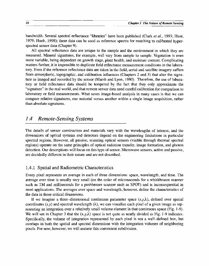
bandwidth. Several spectral reflectance "libraries" have been published (Clark et al., 1993; Hunt, 1979; Hook, 1998); these data can be used as reference spectra for matching to calibrated hyper- spectral sensor data (Chapter 9).
All spectral reflectance data are unique to the sample and the environment in which they are measured. Mineral signatures, for example, will vary from sample to sample. Vegetation is even more variable, being dependent on growth stage, plant health, and moisture content. Complicating matters further, it is impossible to duplicate field reflectance measurement conditions in the labora- tory. Even if the reference reflectance data are taken in the field, aerial and satellite imagery suffers from atmospheric, topographic, and calibration influences (Chapters 2 and 3) that alter the signa- ture as imaged and recorded by the sensor (Marsh and Lyon, 1980). Therefore, the use of labora- tory or field reflectance data should be tempered by the fact that they only approximate the "signature" in the real world, and that remote sensor data need careful calibration for comparison to laboratory or field measurements. What saves image-based analysis in many cases is that we can compare relative signatures, one material versus another within a single image acquisition, rather than absolute signatures.
1.4 Remote-Sensing Systems
The details of sensor construction and materials vary with the wavelengths of interest, and the dimensions of optical systems and detectors depend on the engineering limitations in particular spectral regions. However, all passive, scanning optical sensors (visible through thermal spectral regions) operate on the same principles of optical radiation transfer, image formation, and photon detection. Our descriptions will focus on this type of sensor. Microwave sensors, active and passive, are decidedly different in their nature and are not described.
1.411 Spatial and Radiometric Characteristics
Every pixel represents an average in each of three dimensions: space, wavelength, and time. The average over time is usually very small (on the order of microseconds for a whiskbroom scanner such as TM and milliseconds for a pushbroom scanner such as SPOT) and is inconsequential in most applications. The averages over space and wavelength, however, define the characteristics of the data in those critical dimensions.
If we imagine a three-dimensional continuous parameter space (x,y~L), defined over spatial coordinates (x,y) and spectral wavelength (Z.), we can visualize each pixel of a given image as rep- resenting an integration over a relatively small volume element in that continuous space (Fig. 1-9). We will see in Chapter 3 that the (x,y)~) space is not quite as neatly divided as Fig. 1-9 indicates. Specifically, the volume of integration represented by each pixel is not a well-defined box, but overlaps in both the spatial and spectral dimensions with the integration volumes of neighboring pixels. For now, however, we will assume this convenient subdivision.

1.4 Remote-Sensing Systems 17
0 . 5 ~ , , , I ' ' ' ' ' ' I ' ' ' .I ' ' ' _ : \ i i -
. . . . . 1 , ~ . . ' . _ . \ ~ . ~ . ~ . ~ - K e n t u c k y B l u e G r a s s - 0 . 4 ~ . . . . . . . . . . -/; • - ~ , : - , ~ ~ ......... - R e d F e s c u e G r a s s ]
j : :: ~ . . . . . . . . . P e r e n n i a l R y e G r a s s
................ :t i .... . . . . . . . . . . . . . . . . . . . . . . . . . . i ..... f ' ', . . . . . . . . . . . . . . . . . ~ . . . . . . . . . . . . . . . . . . . . . . . . . i . . . . . . . . . . . . . . . . . . . . . . -
0 . 2 , . . . . . . . . . . . . . . . . . . . . . . . . r - ' - --'-"-,- . . . . . . . . . . . . _
0 . 1 . . . . . . . . . . . . . . . 1 ~. : ~ : - ,~ , L 7 . . . . . . . . . . . . . . . . . . . . . . . ~ . . . . . .
~ ~ _
i - 0 J J i I i i I I i I i I i i i I
4 0 0 8 0 0 1 2 0 0 1 6 0 0 2 0 0 0 2 4 0 0
w a v e l e n g t h ( n m )
. . . . . . . . . . . . . . . . . . . . . . . ~ ~ . , z 2 x . . . . . . . . . . . . . . . . . . - - W h e a t ....
0 . 5 b /if.: ~ ~ - S u g a r B e e t s - t
0 . 4
0 . 3
0 . 2
0 . 1
° f-, ~', , , , , ~ , - - - ; - ~ 4 0 0 8 0 0 1 2 0 0 1 6 0 0 2 0 0 0 2 4 0 0
w a v e l e n g t h ( n m )
FIGURE 1-7. Example vegetation spectral reflectance curves (Bowker et al., 1985). The curves in the upper graph show variability among three types of grasses; even under relatively well-controlled laboratory conditions, the reflectance of corn leaves has been found to vary as much as :d 7% near the reflectance edge at 0.67pm (Landgrebe, 1978).

18 Chapter I The Nature of Remote Sensing
0 . 6
0 .5
0 . 4
0 .3
0 . 2
0 .1
_ I I I I I I I I I I 1 I I I I . ~
_ -
- i / " i ", i i -
. . . . . . . : . . . . _ 7 . . . . . . . . . .::.._._-. . . . . . . . . . . . . . . . . . . . . .,,~ . . . . . . . . . . . . . - . . . . . -~ . . . . . ~ . . . . . . . . . . . . . . . . ~ . . . . . . . . . ~ . . . . . . . . . . . . . . . . . . . . . . . -5_
_~----
_- / Wet Red Clay (20% water) i _-
0 - i I I i i i I ~ i I I i i i I i i i -
4 0 0 800 1200 1600 2 0 0 0 2 4 0 0
w a v e l e n g t h (nm)
1 ~ ~ , , I ' ' ' I ' ' ' ' ' ' ' ' '
~ 0 . 6 ............... ::"i:--: ..................... ! ........... ! , ...... :-" . . . . . . . . . . . . . . . . . . . . : : -
' .
~ 0 . 4
~ - - B u d d ' m g t ° n i t - e G D S 8 5 ...... , i - - - ~ ...... ....... , , ~
0 . 2 ~ ~ ........ • . D°I0miteKaolinite C M 9 HS 102 .......... i ...... i ..............
0 i , , I , , , i , , , 4 0 0 800 1200 1600 2 0 0 0 2 4 0 0
w a v e l e n g t h (nm)
FIGURE 1-8. Example mineral spectral reflectance curves for clay (top) and several alteration minerals (bottom) (Bowker et al., 1985; Clark et al., 1993). The presence o f liquid water in any material generally
lowers the reflectance; for a theory o f this effect, see Twomey et al., 1986.

1.4 Remote-Sensing Systems 19
band 4 50 3 . ~ TM b a n ~ A V I R I S
1
-~ 900 900
\ \ wavelength " - ~ ~ ~ ' ~ wavelength (nm) (nm) X
400 40O
FIGURE 1-9. Comparison of the spatial and spectral sampling of the Landsat TM and AVIRIS in the VNIR spectral range. Each small rectangular box represents the spatial-spectral integration region of one image pixel. The TM samples the spectral dimension incompletely and with relatively broad spectral bands, while AVIRIS has relatively continuous spectral sampling over the VNIR range. AVIRIS also has a somewhat smaller GSI (20m) compared to TM (30m). This type of volume visualization for spatial-spectral image data is called an "image cube" (Sect. 9.9.1).
The grid of pixels that constitutes a digital image is achieved by a combination of scanning in the cross-track direction (orthogonal to the motion of the sensor platform) and by the platform motion along the in-track direction (Fig. 1-10) (Slater, 1980). A pixel is created whenever the sen- sor system electronically samples the continuous data stream provided by the scanning. A line scanner uses a single detector element to scan the entire scene. Whiskbroom scanners, such as the Landsat TM, use several detector elements, aligned in-track, to achieve parallel scanning during each cycle of the scan mirror. A related type of scanner is the paddlebroom, exemplified by AVHRR and MODIS, with a two-sided mirror that rotates 360 °, scanning continuously cross-track. A signif- icant difference between paddlebroom and whiskbroom scanners is that the paddlebroom always scans in the same direction, while the whiskbroom reverses direction for each scan. Pushbroom scanners, such as SPOT, have a linear array of thousands of detector elements, aligned cross-track, which scan the full width of the collected data in parallel as the platform moves. For all types of scanners, the full cross-track angular coverage is called the Field Of View (FOV) and the corre- sponding ground coverage is called the Ground-projected Field Of View (GFOV). 9
9. Also called the swath width, or sometimes, the footprint of the sensor.

20 Chapter 1 The Nature of Remote Sensing
line scanner whiskbroom scanner
in-track ~ ~ " ' " a :
GFOV ~ ~ ETM+ GOES
AVHRR pushbroom scanner MODIS
MSS
TM
ALl
IKONOS
MTI
QuickBird SPOT
FIGURE 1-10. Definition of basic scanner parameters and depiction of three scanning methods, with specific examples of whiskbroom and pushbroom scanners. The solid arrows represent motion relative to a stationary earth. In reality, the earth is rotating during the scanning process, approximately in the cross- track direction since most satellite remote-sensing systems are in a near-polar orbit. This results in a east- west skew in the surface coverage over the full scene.
The spacing between pixels on the ground is the Ground-projected Sample Interval (GSI). The cross-track and in-track GSIs are determined by the cross-track and in-track sampling rates, respectively, and the in-track platform velocity. It is common practice to design the sample rates so that the GSI equals the Ground-projected Instantaneous Field of View (GIFOV), 1° the geometric projection of a single detector width, w, onto the earth's surface (Fig. 1-11 and Fig. 1-12). Thus, the GIFOVs of neighboring pixels will abut, both in-track and cross-track. The in-track GSI is deter- mined by the necessary combination of platform velocity and sample rate (pushbroom) or scan velocity (line and whiskbroom) to match the in-track GIFOV at nadir. Some systems have a higher cross-track sample rate that leads to overlapping GIFOVs, e.g. the Landsat MSS and the AVHRR KLM models. This cross-track "over-sampling" results in some improvement in the data quality.
10.Also called the Ground Sample Distance (GSD).

1.4 Remote-Sensing Systems 21
one detector elemant focal plane width = 14 /~
/
focal lengthf image space
optics
W O altitude H object space
GIFOV ~ i ~ /
Earth's surface
FIGURE 1-11. Simple geometric description of a single detector element in the focal plane of an optical sensor. The sizes of w and fare greatly exaggerated relative to H for clarity. Likewise for the optics (which, more often than not, would be a series of curved mirrors, possibly with multiple, folded optical paths). Angular parameters, such as the IFOV, are the same in image and object space in this model, but linear dimensions are related by the magnification f/H between the two spaces. Everything in this diagram is assumed stationary and in a nadir view; with scan, sensor platform, and earth motion, the GIFOV moves during the integration time of the detector, resulting in an effective GIFOV somewhat larger than shown. Also, as the scan proceeds off-nadir, the effective GIFOV increases (sometimes called "pixel growth") from oblique projection onto the earth. These effects are discussed in Chapter 3.
The GSI is determined by the altitude of the sensor system H, the sensor's focal length, f, and the inter-detector spacing (or spatial sample rate as explained previously). If the sample rate is equal to one pixel per inter-detector spacing, the relation for the GSI at nadir, i.e., directly below the sensor, is simply,
H inter-detector spacing GSI = inter-detector spacing × - = (1-1)
f m
where f /H is the geometric magnification, m, from the ground to the sensor focal plane. 11 As we mentioned, the inter-detector spacing is usually equal to the detector width, w.
11.Since f<< H, m is much less than one.

22 Chapter 1 The Nature of Remote Sensing
typical sensor
GIFOV
GSI I '
+ + , | |
! |
. . . . . + . . . . . . i
| |
|
+ + , + : ! i
in-track I
Landsat MSS, AVHRR
cross-track cross-track
+ + + |
- . . + - + - . i
|
| | |
+ + , .+ | | |
|
_ _ _ ~ m . L . _ ~ m . , . . _ _ _
in-track I
y
FIGURE 1-12. The relationship between GIFOV and GSl for most scanning sensors and for the Landsat MSS and AVHRR. Each cross is a pixel. For MSS, the cross-track GSI was 57m and the GIFOV was 80m, resulting in 1.4 cross-track pixels/GIFOV. Similarly, the AVHRR KLM models have 1.36 cross-track pixels/ GIFOV. The higher cross-track sample density improves data quality, but also increases correlation between neighboring pixels and results in more data collected over the GFOV.
The GIFOV depends in a similar fashion on H, f, and w. System design engineers prefer to use the Instantaneous Field o f View (IFOV), defined as the angle subtended by a single detector element on the axis of the optical system (Fig. 1-11),
I F O V = 2 atan(2j ) _~wf (1-2)
The IFOV is independent of sensor operating altitude, H, and is the same in the image and the object space. It is a convenient parameter for airborne systems where the operating altitude may vary. For the GIFOV, we therefore have,
. _ _ _w G I F O V = 2Htan = w x f m
The GSI and GIFOV are found by scaling the inter-detector spacing and width, respectively, by the geometric magnification, m. Users of satellite and aerial remote-sensing data generally (and justifi- ably) prefer to use the GIFOV, rather than the IFOV, in their analyses. Sensor engineers, on the other hand, often prefer the angular parameters FOV and IFOV because they have the same values in image and object space (Fig. 1-11).

1.4 Remote-Sensing Systems 23
The detector layout in the focal plane of scanners is typically not a regular row or grid arrange- ment. Due to sensor platform and scan mirror velocity, various sample timings for bands and pixels, the need to physically separate different spectral bands, and the limited area available on the focal plane, the detectors are often in some type of staggered pattern as depicted in Fig. 1-13 to Fig. 1-16.
The sensor collects some of the electromagnetic radiation (radiance 12) that propagates upward from the earth and forms an image of the earth's surface on its focal plane. Each detector integrates the energy that strikes its surface (irradiance 13) to form the measurement at each pixel. Due to sev- eral factors, the actual area integrated by each detector is somewhat larger than the GIFOV-squared (Chapter 3). The integrated irradiance at each pixel is converted to an electrical signal and quan- tized as a integer value, the Digital Number (DN). 14 As with all digital data, a finite number of bits, Q, is used to code the continuous data measurements as binary numbers. The number of discrete DNs is given by,
NDN = 2 Q (1-4)
and the DN can be any integer in the range,
DNrange = [ 0, 2 Q - 1 ] . (1-5)
The larger the value of Q, the more closely the quantized data approximates the original continuous signal generated by the detectors, and the higher the radiometric resolution of the sensor. Both SPOT and TM have 8 bits per pixel, while AVHRR has 10bits per pixel. To achieve high radiomet- ric precision in a number of demanding applications, the EOS MODIS is designed with 12bits per pixel, and most hyperspectral sensors use 12bits per pixel. Not all bits are always significant for science measurements, however, especially in bands with low signal levels or high noise levels.
In summary, a pixel is characterized, to the first order, by three quantities: GSI, GIFOV, and Q. These parameters are always associated with the term "pixel" Whenever there may be confusion as to what is meant between the GSI and GIFOV, "pixel" should be reserved to mean the GSI.
Discrete multispectral channels are typically created in an optical sensor by splitting the optical beam into multiple paths and inserting different spectral filters in each path or directly on the detec- tors. Some hyperspectral sensors, such as HYDICE, use a two-dimensional array of detectors in the focal plane (Fig. 1-17). A continuous spectrum is created across the array by an optical component such as a prism or diffraction grating. For HYDICE, the detector array has 320 elements cross-track and 210 in-track. The cross-track dimension serves as a line of pixels in a pushbroom mode, while the optical beam is dispersed over wavelength by a prism along the other direction (in-track) of the array. Therefore, as the sensor platform (an aircraft in the case of HYDICE) moves in-track, a full
12.Radiance is a precise scientific term used to describe the power density of radiation; it has units of W-m -2- sr-l-~tm-1, i.e., watts per unit source area, per unit solid angle, and per unit wavelength. For a thorough dis- cussion of the role of radiometry in optical remote sensing, see Slater (1980) and Schott (1996).
13.Irradiance has units of W-m-2-~tm -1. The relationship between radiance and irradiance is discussed in Chapter 2.
14.Also known as Digital Count.

24 Chapter I The Nature of Remote Sensing
band 8 [] [] [] [] [] [] [] [] [] [] [] [] [] [] [] []
1 2
-1 [3 -1D N D Z] E] FI n -1 [3 iZ] D Z] F1 i -1N
3 E] r-1D 3 D D D --1D [3 D
D r-1 prime focal plane (Si)
3 4
N
D N
r--I
N
[3 f-I I-1
i I 7 5 6
I ~ [3 ~-~ I E] D ~-~ I D ~ ~-~ I Fq D ~-~ I D D
G [---] I D
I D D [---]
I cold focal plane (InSb and (IIgCdTe) I
I> cross-track
t in-track
FIGURE 1-13. Focal plane detector layout of ETM+. The prime focal plane contains the lOm (GIFOV) panchromatic and 30m VNIR bands with silicon (Si) detectors; the cold focal plane is cooled to reduce detector noise and contains the 30m SWIR bands with Indium-Antimonide (InSb) detectors and the 60m LWIR bands with Mercury-Cadmium-Telluride (HgCdTe) detectors. As the scan mirror sweeps the image across the focal planes in the cross-track direction, data are acquired in all bands simultaneously; electronic sample timing is used to correct the cross-track phase differences among pixels. The photographs of the focal plane assemblies indicate the detector array's actual s i ze-a few millimeters. (Raytheon photographs courtesy of Ken J. Ando.)

1.4 Remote-Sensing Systems 25
band 10 9 8
I - -
, ~ - - - _
I
11
i
VIS focal plane (Si)
1
I
12 I 19 18
!
cross-track
in-track
13 2 1 14
NIR focal plane (Si)
15 16 17
| |
- H -
ZM- , ,
ZU-
FIGURE 1-14. Detector layout of the MODIS uncooled VIS and NIR focal planes. The arrays appear dark in both cases because of anti-reflection optical coatings. The NIR focal plane contains the 250m red and NIR bands I and 2 that are used mainly for land remote sensing. The double columns of detectors in bands 13 and 14 employ Time Delay Integration (TDI) to increase signal and reduce noise levels for dark scenes such as oceans. The data from one column are electronically delayed during scanning to effectively align with the data from the other column, and then the two sets of data are summed, in effect increasing the integration time at each pixel in bands 13 and 14. (Raytheon photographs courtesy of Ken J. Ando and John Vampola.)
26 Chapter I The Nature of Remote Sensing
band i
26 25 24 7 6 5 20 21 22 23 I 30 29 28 27 33 34 35 36 31 32
_ _ _ _ _ _ J _
_ _ _ i 7_
L__._ _ _
7 - - -
i
SWIR/MWIR focal plane (PV HgCdTe) i
l - -
i
i ! -
I l -
i , - -
I
I -
i
I I I I (PV HgCdTe) ] (PC HgCdTe)
LWIR focal plane
I I cross-track
in-track
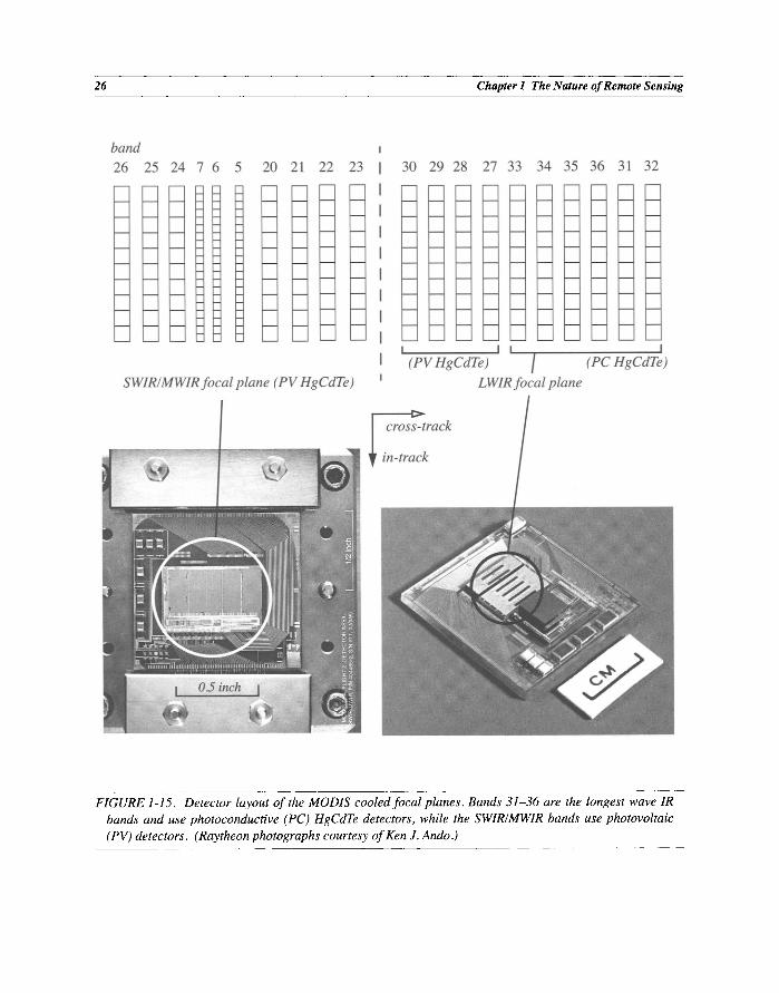
FIGURE 1-15. Detector layout of the MODIS cooled focal planes. Bands 31-36 are the longest wave IR bands and use photoconductive (PC) HgCdTe detectors, while the SWIR/MWIR bands use photovoltaic (PV) detectors. (Raytheon photographs courtesy of Ken J. Ando.)

1.4 Remote-Sensing Systems 27
I
S C A 3 I : [
S C A 4 I S C A 2 i
I- !
S C A 1
SCA detail:
b a n d
p a n
1
l p
VNIR 2
(Si) 3
4
4p
cross-track
in-track
pixels 0, 2, 4 . . . . oooooa
aaaaaa
1,3 5 . . . .
- - ." "., 0 , 2 , 4 . . . . . . . . ,..-_--'+ [] [] [] []
. . - . ~ D D D D " - 1 3 , 5 . . . .
s
960 pixels/line
320 pixels/line
5p . 0 , 2 , 4 . . . . S WIR "- [] [] [] []
5 - " ' " [] [] [] [] (HgCdTe) 320 pixels/line - " D D D D
7 - " []DDD 1 , 3 , 5 . . . . .
FIGURE 1-16. The four sensor chip assemblies (SCAs) in the ALl. The even- and odd-numbered detectors in each band are in separate rows on the SCA; the phase difference is corrected by data processing. The double rows of detectors in the SWIR bands 5p (the "p" denotes a band that does not correspond to a ETM+ band), 5, and 7 allow TDI for higher signal-to-noise (SNR) (see also Fig. 1-14 for an explanation of TDI). There are a total of 3850 panchromatic detectors and 11,520 multispectral detectors on the four SCAs. The pixels resulting from overlapping detectors between SCAs are removed during geometric processing of the imagery (Storey et al., 2004).
28 Chapter 1 The Nature of Remote Sensing
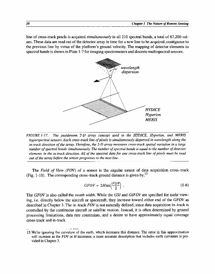
line of cross-track pixels is acquired simultaneously in all 210 spectral bands, a total of 67,200 val- ues. These data are read out of the detector array in time for a new line to be acquired, contiguous to the previous line by virtue of the platform's ground velocity. The mapping of detector elements to spectral bands is shown in Plate 1-7 for imaging spectrometers and discrete multispectral sensors.
~ w a v e l e n g t h ersion
YDICE Hyperion MERIS
FIGURE 1-17. The pushbroom 2-D array concept used in the HYDICE, Hyperion, and MERIS hyperspectral sensors. Each cross-track line of pixels is simultaneously dispersed in wavelength along the in-track direction of the array. Therefore, the 2-D array measures cross-track spatial variation in a large number of spectral bands simultaneously. The number of spectral bands is equal to the number of detector elements in the in-track direction. All of the spectral data for one cross-track line of pixels must be read out of the array before the sensor progresses to the next line.
The Field o f View (FOV) of a sensor is the angular extent of data acquisition cross-track (Fig. 1-10). The corresponding cross-track ground distance is given by, 15
GFOV = 2Htan(-~-~ . (1-6)
The GFOV is also called the swath width. While the GSI and GIFOV are specified for nadir view- ing, i.e. directly below the aircraft or spacecraft, they increase toward either end of the GFOV as described in Chapter 3. The in-track FOV is not naturally defined, since data acquisition in-track is controlled by the continuous aircraft or satellite motion. Instead, it is often determined by ground processing limitations, data rate constraints, and a desire to have approximately equal coverage cross-track and in-track.
15.We're ignoring the curvature of the earth, which increases this distance. The error in this approximation will increase as the FOV or H increases; a more accurate description that includes earth curvature is pro- vided in Chapter 3.

1.4 Remote-Sensing Systems 29
m
| 320 columns (pixels) 12.8mm
210 rows (bands 1--206) 8.4mm
cross-track
in-track
InSb detector array
FIGURE 1-18. The 2-D detector array layout used in HYDICE. Each detector element is 40pro on a side, and there are 67,200 detectors in the array. The array is segmented into three regions (400-1000, 1000- 1900 and 1900-2500nm) with different electronic gains (Chapter 3) to compensate for different solar energy levels across the VSWIR spectrum (Fig. 1-6). (Photo courtesy of Bill Rappoport, Goodrich Electro- Optical Systems.)

30 Chapter I The Nature of Remote Sensing
Sensors with multiple detectors per band, such as whiskbroom and pushbroom scanners, require relative radiometric calibration of each detector. The MSS had 6 detectors in each of 4 bands, for a total of 24, and the TM has 16 detectors in each of the 6 non-TIR bands (30m GS1), plus 4 in band 6 (120m GSI), for a total of 100 detectors. The Landsat-7 ETM+ has, in addition to the normal TM complement, 32 detectors in the panchromatic band (15m GS1) and 8 in band 6 (60m GSI), making a total of 136 detectors. Each detector is a discrete electronic element with its own particular responsitivity characteristics, so relative radiometric calibration among detectors is particularly important. Errors in calibration lead to cross-track "striping" and "banding" noise in these systems, which can be quite visible artifacts. A pushbroom system has a very large number of cross-track detector elements (6000 in the SPOT panchromatic mode, averaged to 3000 in the multispectral mode), requiring proportionally more calibration effort. The most severe calibration requirements are for 2-D array hyperspectral sensors such as HYDICE--its focal plane has 67,200 individual detector elements within a single array (Fig. 1-18).
Line and whiskbroom scanners clearly have many dynamic motions occuring during scene acquisition (mirror rotation, earth rotation, satellite or aircraft roll/pitch/yaw) and consequently require complex post-processing to achieve accurate geometry. This can be done to a high level, however, as exemplified by the high quality of Landsat TM imagery. The geometry of a pushbroom scanner such as SPOT or ALI is comparatively simple, since scanning is achieved by the detector motion in-track. Factors such as earth rotation and satellite pointing during image acquisition affect the image geometry in any case. A comparison of ETM+ and ALI geometric performance is shown in (Fig. 1-19).
The total time required to "build" an image of a given in-track length depends on the satellite ground velocity, which is about 7 km/sec for low altitude, earth-orbiting satellites. A full TM scene therefore requires about 26 seconds to acquire, and a full SPOT scene about 9 seconds. The number of detectors scanning in parallel directly affects the amount of time available to integrate the incom- ing optical signal at each pixel. Pushbroom systems therefore have an advantage because all pixels in a line are recorded at the same time (Fig. 1-10). If there were no satellite motion, the radiometric quality of the image would increase with increased integration time, because the signal would increase relative to detector noise. With platform motion, however, longer integration times also imply greater smearing of the image as it is being sensed, leading to reduced spatial resolution. This effect is more than offset by the increased signal-to-noise ratio of the image (Fig. 1-20).
1.4.2 Spec t ra l Cha rac t e r i s t i c s
The spectral location of sensor bands is constrained by atmospheric absorption bands and further determined by the reflectance features to be measured. If a sensor is intended for land or ocean applications, atmospheric absorption bands are avoided in sensor band placement. On the other hand, if a sensor is intended for atmosphere applications, it may very well be desirable to put spec- tral bands within the absorption features. An example of a sensor designed for all three applica- tions, MODIS collects spectral images in numerous and narrow (relative to ETM+) wavelength

1.4 Remote-Sensing Systems 31
ETM+ Level 1G band I ALl Level 1R band 2
FIGURE 1-19. Visual comparison of ETM+ whiskbroom and ALl pushbroom imagery acquired on July 27, 2001, of center-pivot irrigated agricultural fields near Maricopa, Arizona. The ALl Level 1R image, which has no geometric processing, depicts the circular shape of the center pivot irrigated fields more accurately than does the ETM+ Level 1G image, which has geometric corrections applied with nearest-neighbor resampling (Chapter 7). The pushbroom geometry of ALl is inherently better than that of a whiskbroom scanner like ETM+. Also, the superior SNR characteristics of ALl produces an image that shows somewhat better detail definition and less "noise." (ETM+ image provided by Ross Bryant and Susan Moran of USDA-ARS, Southwest Watershed Research Center, Tucson.)
bands from the visible through the thermal infrared. The MODIS spectral band ranges are plotted in Fig. 1-21. All of the 36 bands are nominally co-registered and acquired at nearly the same time dur- ing scan mirror rotation.
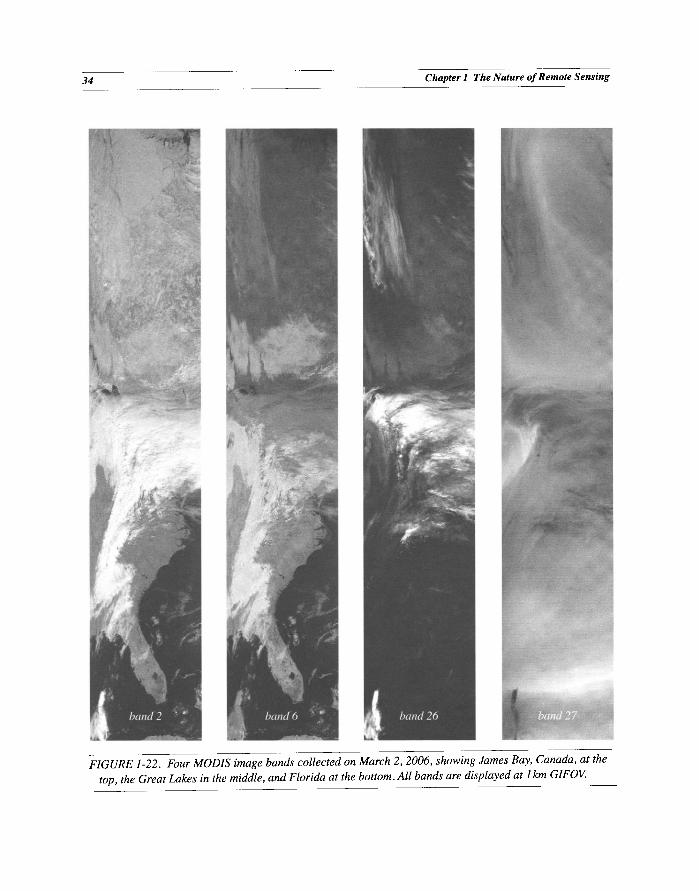
The diversity of information in different bands is illustrated in Fig. 1-22 (all bands are displayed at 1 km GIFOV). These are Direct Broadcast (DB) data received at the USGS National Center for EROS in Sioux Falls, South Dakota. DB data are processed rapidly without the full ancillary data used for archived MODIS data. This winter image shows ice and snow in St. James Bay and Can- ada, thick clouds over the northeastern United States and clear skies along the eastern coast down to Florida. Band 2 is the NIR, band 6 is a band designed to distinguish ice and snow from clouds (ice and snow have low reflectance relative to clouds in this band), band 26 is designed to detect cirrus clouds, and band 27 senses mid-tropospheric water vapor. Note that the Earth's surface is not visi- ble in bands 26 and 27 because they are in major atmospheric absorption bands (Fig. 1-21).

32 Chapter 1 The Nature of Remote Sensing
. . . . ~ i ¸ •~•
f
ETM+ pan ALl pan
FIGURE 1-20. Visual comparison of ETM+ whiskbroom and ALl pushbroom panchromatic imagery of an area in Alaska acquired by ETM+ on November 27, 1999, and ALl on November 25, 2000 (Storey, 2005). The solar irradiance level was quite low because of the high latitude of the site 'and the winter acquisition dates, and both images have been strongly contrast stretched for visibility. The ALl clearly produced a better image with less "noise," largely because of the superior signal-to-noise properties of its pushbroom sensor.
1.4.3 Temporal Characteristics
One of the most valuable aspects of unmanned, near polar-orbiting satellite remote-sensing systems is their inherent repeating coverage of the same area on the earth. Regular revisits are especially important for monitoring agricultural crops; in fact, temporal signatures can be defined for certain crop types in different regions of the world and used to classify them from multitemporal images (Haralick et al., 1980; Badhwar et al., 1982). Other applications for multitemporal data are change detection of both natural and cultural features and monitoring of the atmosphere and oceans.
Many remote sensing satellites, including Landsat, AVHRR, and SPOT, are in sun-synchronous orbits which means that each always passes over the same spot on the ground at the same local time. The interval between revisits depends solely on the particulars of the satellite orbit for sensors that have a fixed view direction (nadir), such as the Landsat TM. If more than one system is in orbit

1.4 Remote-Sensing Systems 33
' '- . . . . . . ' . . . . . . . I . . . . . . : . . . . . . i . . . . . . '_ . . . . . . . . . . . . . ' . _ . ~ i i i i i i i i i i i i i . . . . . . . . . . . . . ~ . . . . . . . . . ~9 . . . . . . . . . . . i . . . . . . . . .
. . . . . . . . . . . . . . . . . . . . . . . . . . i . . . . . . . . . . . ] 8 . . . . . . . . . . . . i . . . . . . . . .
. . . . . . . . . . . . . . . . . . . . . . . . . . i . . . . . - - . - 1 7 . . . . . . . . . . . . . ~ . . . . . . . . .
1 6
..................... 1 4 ! ' ......................... i ......... | . . . . . . . . . . . . . . . . . . . 1 3 . . . . . . . . . . . . . . . . . . . . . . . . . . . . . . i . . . . . . . . .
. . . . . . . . . . . 1 2 . . . . . . . . . . . i . . . . . . . . . . . . . . . . . . . . . . . . . . . i . . . . . . . . .
' . . . . . . . 11 . . . . . . . . . . . . . :: . . . . . . . . . . . . . . . . . . . . . . . . . . . i . . . . . . . . .
. . . . . . . l o . . . . . . . . . . . . . . . :: . . . . . . . . . . . . . . . . . . . . . . . . . . . i . . . . . . . . .
- - - 9 . . . . . . . . . . . . . . . . . . . . :: . . . . . . . . . . . . . . . . . . . . . . . . . . . i . . . . . . . . .
___i ................................................. i---5-- . . . . . . . . . . . 4 . . . . . . . . . . . . i . . . . . . . . . . . . . . . . . . . . . . . . . . . ~ ..
- - - ~ - 3 - . . . . . . . . . . . . . . . . . . . . . . . . . . . . . . . . . . . . . . . . . . . . i . . . . . . . . . "
. . . . . . . . . . . . . . . . . . . . . . . . . . :: . . . . 2 . . . . . . . . . . . . . . . . . . ~ . . . . . . . . .
. . . . . i . . . . . . i - , ~ . . . . :: . . . . . . ; . . . . . . i . . . . . . i . . . . . . i . . . . . . i---
0 . 4 0 . 8 1 . 2
- 2 6 - - ' . . . . . . ! . . . . . . . . . . . . . . . . . ? . . . . . . . . . . . '- . . . . . .
............. i ............. i ~ s v s w ~ -
1.6 2 2.4
w a v e l e n g t h ( k t m )
....... - ' H i / ' ' 3] 4 - - iiiiiiiiiiiiiiii iiiiiiiiiiiiiiiiiiiiiiiiiiiiiiiiiiil. ~ ..... , ........... J ..... i ...................... ~ .......... ~---
_ _ ~ . . . . . . . . . . . . . . . . . ~ . . . . . i . . . . . . . . . . . . . . , 3 2 . . . . . . . . . . . . . . . .
....................... - . . . . . ! . . . . . . . . . . . ~ . . . . . "-- 3 1 . . . . . . . ~ . . . . . . . . . . . . . . . . . . . ~ ' - " - - ' - ' - ~ - i m :
~- ~ i i ~ i i ~ i i i i ~ i i i i l J i ~ i i i i i i ~ i i i i i ~ ................. - i -!
2 3 ~ . . . . . . . . . . . . . . . . . . . . . . . ! . . . . . . . . . . . . . . . . . . . . . . ! . . . . . . . . . . . . . . . . . . . .
. . . . . : 2 - m ~ ~ . . . . . . i . . . . . . . . . . . . . . . . i . . . . . . . . . . . . . . . . . . . . . . i . . . . . . . . . . . . . . . . . . . .
. . . . . : 1 . . . . . . . . . . . . . . . . . . . . . ~ . . . . . i . . . . . . . . . MODIS'MWIR,LWIR-
~ o N ~ ... . . . . i . . . . . . . . . ; d i : , ..... i : ~ 2 . 5 4 . 5 6 . 5 8 . 5 1 0 . 5 1 2 . 5 1 4 . 5
w a v e l e n g t h ( g r n )
FIGURE 1-21. Spectral ranges for the 36 MODIS bands. The shaded areas are the major atmospheric absorption bands. Note that bands 1 and 2, the 250m GSI land sensing bands, straddle the vegetation reflectance "red edge" (Fig. 1-7). Bands 26, 27, 28, and 30, all located within atmospheric absorption bands, are designed to measure atmospheric properties. All bands were located to optimize measurement of specific land, ocean, and atmospheric features (Table 1-2).
34 Chapter I The Nature of Remote Sensing
FIGURE 1-22. Four MODIS image bands collected on March 2, 2006, showing James Bay, Canada, at the top, the Great Lakes in the middle, and Florida at the bottom. All bands are displayed at I km GIFOV.

1.4 Remote-Sensing Systems 35
at the same time, it is possible to increase the revisit frequency. The SPOT systems are pointable and can be programmed to point cross-track to a maximum of _+26 ° from nadir, which allows a sin- gle satellite to view the same area more frequently from different orbits. The high resolution com- mercial satellites, IKONOS and QuickBird, are even more "agile" i.e. they can point off-nadir within a short time. They can thus obtain two in-track views at different angles of the same area, within minutes of each other, to make a stereo pair. Without pointing, their revisit times are 1 to 3 days, depending on the latitude (more frequent at high latitudes). Manned systems, such as the Space Shuttle, which has carried several experimental SAR and other remote-sensing systems, and the International Space Station, have non-polar orbits which allow less regular revisit cycles. Some example revisit times of remote sensing satellites are given in Table 1-5. An example multitemporal image series is shown in Plate 1-8.
TABLE 1-5. Revisit intervals and equatorial crossing times for several satellite remote sensing systems. The specifications assume only one system in operation, with the exception of the AVHRR, which normally operates in pairs, and the two MODIS systems, allowing morning and afternoon viewing of the same area in one day. The GOES is in a geostationary orbit and is always pointed at the same area of the earth. Equatorial crossing times are only approximate, as they change continually by small amounts and orbit adjustments are needed periodically.
system
AVHRR
revisit interval
1 day (one system) 7 hours (two systems)
daylight equatorial crossing time
7:30 A.M. 2:30 P.M.
GOES 30 minutes NA
IKONOS minutes (same orbit), 1-3 days (pointing) 10:30 A.M.
IRS-1A, B 22 days 10:30 A.M.
Landsat 18 days (L-l, 2, 3)/16 days (L-4, 5, 7) 9:30 A.M./10:15 A.M.
MODIS 3 hours-1 day 10:30 A.M. descending (Terra) 1:30 P.M. ascending (Aqua)
QuickBird minutes; 1-3 days 10:30 A.M.
SPOT 26 days (nadir only); 1 day or 4-5 days (pointing) 10:30 A.M.
1.4.4 M u l t i - S e n s o r F o r m a t i o n F l y i n g
Since a single sensor cannot make all desired measurements of the Earth and its atmosphere, we must rely on combining data from several sensors to achieve a complete picture for scientific analy- sis. One of the ways to do this is to create a "train" of sensors on different satellites, traveling in the same orbit and separated by short time intervals, similar to planes flying in formation. The initial NASA demonstration of this concept was a morning formation, including Landsat-7 in the lead, EO-1 (1 minute behind Landsat-7), Terra (15 minutes behind), and the Argentine satellite SAC-C
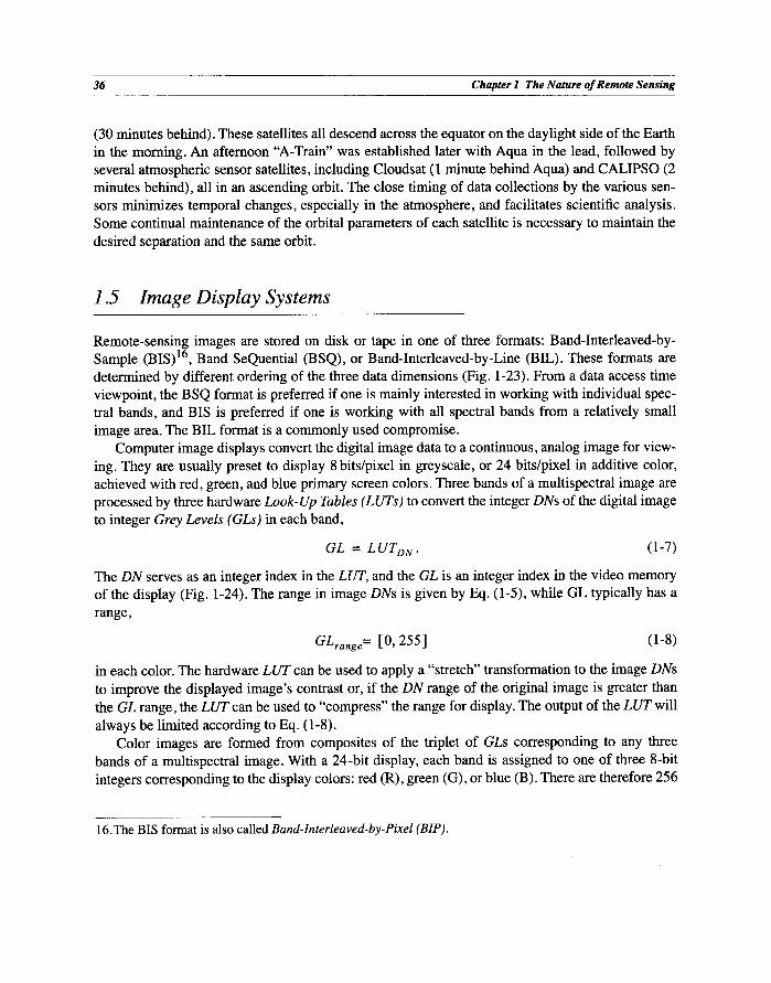
36 Chapter 1 The Nature of Remote Sensing
(30 minutes behind). These satellites all descend across the equator on the daylight side of the Earth in the morning. An afternoon "A-Train" was established later with Aqua in the lead, followed by several atmospheric sensor satellites, including Cloudsat (1 minute behind Aqua) and CALIPSO (2 minutes behind), all in an ascending orbit. The close timing of data collections by the various sen- sors minimizes temporal changes, especially in the atmosphere, and facilitates scientific analysis. Some continual maintenance of the orbital parameters of each satellite is necessary to maintain the desired separation and the same orbit.
1.5 Image Display Systems
Remote-sensing images are stored on disk or tape in one of three formats: Band-Interleaved-by- Sample (BIS) 16, Band SeQuential (BSQ), or Band-Interleaved-by-Line (BIL). These formats are determined by different ordering of the three data dimensions (Fig. 1-23). From a data access time viewpoint, the BSQ format is preferred if one is mainly interested in working with individual spec- tral bands, and BIS is preferred if one is working with all spectral bands from a relatively small image area. The B IL format is a commonly used compromise.
Computer image displays convert the digital image data to a continuous, analog image for view- ing. They are usually preset to display 8 bits/pixel in greyscale, or 24 bits/pixel in additive color, achieved with red, green, and blue primary screen colors. Three bands of a multispectral image are processed by three hardware Look-Up Tables (LUTs) to convert the integer DNs of the digital image to integer Grey Levels (GLs) in each band,
GL = L UTDN . (1-7)
The DN serves as an integer index in the LUT, and the GL is an integer index in the video memory of the display (Fig. 1-24). The range in image DNs is given by Eq. (1-5), while GL typically has a range,
GZrange = [0, 255] (1-8)
in each color. The hardware LUT can be used to apply a "stretch" transformation to the image DNs to improve the displayed image's contrast or, if the DN range of the original image is greater than the GL range, the LUT can be used to "compress" the range for display. The output of the LUT will always be limited according to Eq. (1-8).
Color images are formed from composites of the triplet of GLs corresponding to any three bands of a multispectral image. With a 24-bit display, each band is assigned to one of t~ee 8-bit integers corresponding to the display colors: red (R), green (G), or blue (B). There are therefore 256
16.The BIS format is also called Band-Interleaved-by-Pixel (BIP).

1.5 Image Display Systems 37
E lines 1-8
bands 1-7
BIS or BIP
samples 1-8
bands 1-7
lines 1-8
BSQ BIL
samples 1 - 8 samples 1 - 8 i i I ~ I
-bandsl_7 1 .........
lines 1-8
FIGURE 1-23. The three most common multispectral image formats: BIS, BSQ, and BIL, illustrated with an 8 sample-by-8 line-by-7 band TM image. Note the very low contrast in the TIR band 6 relative to the other bands.
GLs available for each band. Every displayed pixel has a color defined by a triplet of GLs, which we may consider a three-dimensional column vector RGB,17
R G B = [ GLR,GLG,GL~] r . (1-9)
There are 2563 possible R G B vectors, but fewer distinguishable display colors because there are no monitors that can display all of the colors in the color cube. The exact color displayed for a given R G B data vector depends on the phosphor characteristics and control settings of the monitor.
Computer monitors create color in an additive way; that is, a pixel with equal GLs in red, green,
and blue will appear as grey on the screen (if the monitor is properly adjusted); a pixel with equal amounts of red and green, and with no blue, appears as yellow, and so forth. Certain color combina- tions are widely used in remote sensing (Table 1-6). However, since many commonly-used bands are not even in the visible spectrum, color assignment in the display image is arbitrary. The "best"
17.The triplet is conveniently written as a row vector in Eq. (1-9). The superscript T converts it to a column vector by a transpose operation.
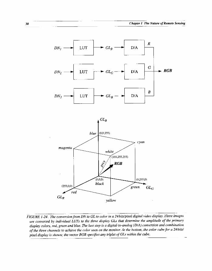
38 Chapter 1 The Nature of Remote Sensing
DN 1
DN 2
DN 3
LUT
LUT
LUT
GL R
GL G
GL B
D/A
D/A
D/A
G RGB
GLB
blue (o,0,255)
magenta ~ ~ cyan
I ~ RGB
(255'~ ~ ~/'a° 2~ [ ~ g r g r e e n GL G
red ~ l ~
GLR yellow
FIGURE 1-24. The conversion from DN to GL to color in a 24bits/pixel digital video display. Three images are converted by individual LUTs to the three display GLs that determine the amplitude of the primary display colors, red, green and blue. The last step is a digital-to-analog (D/A) conversion and combination of the three channels to achieve the color seen on the monitor. At the bottom, the color cube for a 24 bits/ pixel display is shown; the vector RGB specifies any triplet of GLs within the cube.

1.6 Data Systems 39
colors to use are those that enhance the data of interest. The popularity of the Color IR (CIR) type of display derives from its emulation of color IR photography, in which vegetation appears as red because of its relatively high reflectance in the NIR and low reflectance in the visible (Fig. 1-7). Anyone with photointerpretation experience is usually accustomed to interpreting such images. The natural color composite is sometimes called a "true" color composite, but that is misleading as there is no "true" color in remote sensing--natural color is more appropriate for the colors seen by the eye. The bands used to make TM CIR and natural color composites are shown in Plate 1-9.
Single bands of a multispectral image can be displayed as a greyscale image or pseudo-colored by converting each DN or range of DNs to a different color using the display's LUTs. Pseudo- coloring makes it easier to see small differences in DN.
TABLE 1-6. Sensor band mapping to RGB display color for standard color composites. A general false color composite is obtained by combining any three sensor bands.
sensor
composite type
natural color Color IR (CIR)
generic red: green:blue NIR: red: green
ALI 4:3:2 5:4:2
ASTER NA 3:2:1
AVIRIS 30:20:9 45:30:20
Hyperion 30:21:10 43:30:21
MODIS 13:12:9 16:13:12
MSS NA 4:2:1
SPOT NA 3:2:1
TM, ETM+ 3:2:1 4:3:2
1.6 Data Systems
The data volume and technical complexity of modem remote sensing systems dictate that some preprocessing of the data be performed before it is supplied to the science community. The aim of preprocessing is to create a consistent and reliable image database by
• calibrating the image radiometry
• correcting geometric distortions
• removing some types of sensor noise
• formatting to a standard prescription

40 Chapter 1 The Nature of Remote Sensing
The particular types of preprocessing required obviously depend on the sensor's characteristics, since the goal is to remove any undesirable image characteristics caused by the sensor. Since not all data users need, or can afford, the highest degree of correction, various levels of preprocessing are provided as options.
A taxonomy of data products has evolved for major remote-sensing systems along the lines shown in Table 1-7. A generic hierarchy that encompasses these examples is given by four major processing levels
• reformatted raw data
• sensor- corrected data
• geometric corrections
• radiometric corrections
• scene- corrected data
• geometric corrections
• radiometric corrections
• geophysical data
Each level normally requires more ancillary data and processing than the preceding level. Typically, only a small fraction of the total data collected is processed to the higher levels, and the cost to the data customer generally increases with the level of processing. NASA was responsible for Landsat TM data production until that task was assumed by the commercial firm, EOSAT, on September 27, 1985. The levels of processing produced by NASA during the pre-commercialization period are documented (Clark, 1990). In recent years, processing responsibility for Landsat-5 and -7 was returned to the government. The engineering characteristics of the Landsat TM also were described thoroughly in two special journal issues (Salomonson, 1984; Markham and Barker, 1985).
Information extraction from the preprocessed images is generally done by earth science researchers. But, since not all data are processed to the highest level at a central site, the earth scien- tist often must do equivalent processing before information extraction can begin, e.g., co-registra- tion of scenes from different dates or sensors. It is, therefore, important that ancillary calibration data (primarily radiometric and geometric) be included with data supplied to users.
The approach taken in the NASA EOS program has been somewhat different from that used earlier. EOS satellite data, such as that from ASTER and MODIS, are used to produce not only lower level 1A or 1B radiance products, but also higher level products, using production algorithms developed by teams of scientists in their respective fields. Examples are the ASTER AST07 and MODIS MOD09 products for Level 2 surface reflectance and the MODIS Vegetation Index product MOD13. Many higher level EOS products use not only sensor data, but also rely on the results of other product calculations. For example, the MODIS surface reflectance product (MOD09) uses Level 1B MODIS bands 1-7 for radiance values, band 26 to detect cirrus clouds, MOD35 for cloud detection and masking, MOD05 for atmospheric water vapor correction, MOD04 for atmospheric aerosol correction, MOD07 for atmospheric ozone correction, and MOD43 for a coupling term involving the atmosphere and the surface Bi-directional Reflectance Distribution Function (BRDF).

1.6 Data Systems 41
TABLE 1-7. Processing levels for NASA earth remote-sensing systems.
processing system level description
NASA EOS (Asrar and
Greenstone, 1995)
EOSAT TM (EOSAT, 1993)
ETM+
(USGS, 2000)
1A
1B
Reconstructed unprocessed instrument/payload data at full resolu- tion; any and all communications artifacts (e.g., synchronization frames, communications headers) removed.
Reconstructed unprocessed instrument data at full resolution, time- referenced, and annotated with ancillary information, including radiometric and geometric calibration coefficients and georefer- encing parameters (i.e., platform ephemeris) computed and appended, but not applied, to the Level 0 data (or if applied, applied in a manner in which Level 0 data can be fully recovered).
Level 1A data that have been processed to calibrated sensor units (not all instruments will have a Level 1B equivalent; Level 0 data is not recoverable from Level 1B data).
Derived geophysical variables at the same resolution and location as the Level 1 source data.
Level 1 or 2 data or other variables mapped on uniform space-time grid scales, usually with some completeness and consistency.
Model output or results from analyses of lower level data, e.g., 4
variables derived from multiple measurements.
system
Geometric correction and projection to one of 20 map projections and rotation to north-up, using ephemeris data and systematic error models. Relative detector calibration non-thermal bands. UTM, SOM or polar stereographic projection with residual distortions of 200 300m (orbit-oriented product).
precision Map projection using Ground Control Points (GCPs).
terrain Orthographic projection using DEMs.
No radiometric or geometric corrections, but includes all necessary OR
data for radiometric and geometric corrections.
1R Radiometrically corrected for detector gains and offsets.
1G
Radiometrically corrected, resampled for geometric correction and registration to a geographic map projection. Includes satellite, sen- sor scan, and earth geometry corrections, but not topographic cor- rections.
In turn, the MOD09 product is used in generation of the vegetation products MOD 13 and MOD 15,
as well as many other products. Some example MODIS science products are listed in Table 1-8, and two MODIS science products are shown in Plate 1-10.
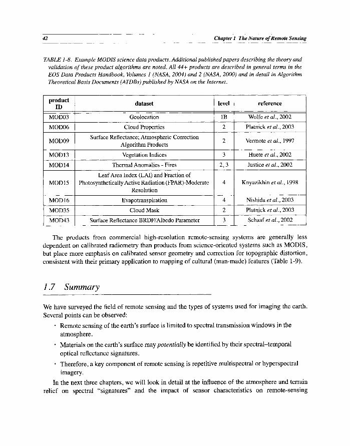
42 Chapter 1 The Nature of Remote Sensing
TABLE 1-8. Example MODIS science data products. Additional published papers describing the theory and validation of these product algorithms are noted. All 44+ products are described in general terms in the EOS Data Products Handbook, Volumes 1 (NASA, 2004) and 2 (NASA, 2000) and in detail in Algorithm Theoretical Basis Documents (ATDBs) published by NASA on the Internet.
product dataset ID
MOD03 Geolocation
MOD06 Cloud Properties
Surface Reflectance; Atmospheric Correction MOD09 Algorithm Products
MOD 13 Vegetation Indices
MOD 14 Thermal Anomalies - Fires
MOD15 Leaf Area Index (LAI) and Fraction of
Photosynthetically Active Radiation (FPAR)-Moderate Resolution
MOD 16 Evapotranspiration
MOD35 Cloud Mask
MOD43 Surface Reflectance BRDF/Albedo Parameter
level reference
1B Wolfe et al., 2002 ,
2 Platnick et al., 2003
2 Vermote et al., 1997
3 Huete et al., 2002
2, 3 Justice et al., 2002
4 Knyazikhin et al., 1998
4 Nishida et al., 2003
2 Platnick et al., 2003
3 Schaaf et al., 2002
The products from commercial high-resolution remote-sensing systems are generally less dependent on calibrated radiometry than products from science-oriented systems such as MODIS, but place more emphasis on calibrated sensor geometry and correction for topographic distortion, consistent with their primary application to mapping of cultural (man-made) features (Table 1-9).
1.7 Summary
We have surveyed the field of remote sensing and the types of systems used for imaging the earth. Several points can be observed:
• Remote sensing of the earth's surface is limited to spectral transmission windows in the
atmosphere.
• Materials on the earth's surface may potentially be identified by their spectral-temporal
optical reflectance signatures.
• Therefore, a key component of remote sensing is repetitive multispectral or hyperspectral
imagery.
In the next three chapters, we will look in detail at the influence of the atmosphere and terrain relief on spectral "signatures" and the impact of sensor characteristics on remote-sensing
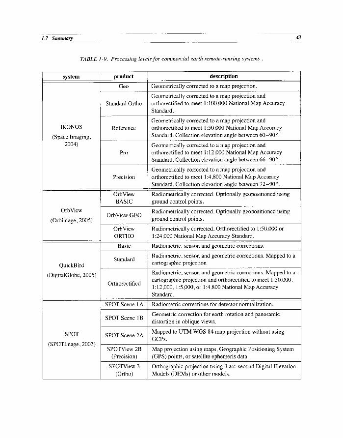
1.7 Summary 43
TABLE 1-9. Processing levels for commercial earth remote-sensing systems.
system product
IKONOS
(Space Imaging, 2004)
Geo
QuickBird
(DigitalGlobe, 2005)
Standard Ortho
Reference
Pro
Precision
description
Geometrically corrected to a map projection.
Geometrically corrected to a map projection and orthorectified to meet 1:100,000 National Map Accuracy Standard.
Geometrically corrected to a map projection and orthorectified to meet 1:50,000 National Map Accuracy Standard. Collection elevation angle between 60-90 ° .
Geometrically corrected to a map projection and orthorectified to meet 1:12,000 National Map Accuracy Standard. Collection elevation angle between 66-90 ° .
Geometrically corrected to a map projection and orthorectified to meet 1:4,800 National Map Accuracy Standard. Collection elevation angle between 72-90 ° .
OrbView Radiometrically corrected. Optionally geopositioned using BASIC ground control points.
OrbView Radiometrically corrected. Optionally geopositioned using OrbView GEO
(Orbimage, 2005) ground control points.
OrbView Radiometrically corrected. Orthorectified to 1:50,000 or ORTHO 1:24,000 National Map Accuracy Standard.
Basic Radiometric, sensor, and geometric corrections.
Radiometric, sensor, and geometric corrections. Mapped to a Standard
cartographic projection
Orthorectified
SPOT Scene 1A
SPOT
(SPOTImage, 2003)
SPOT Scene 1B
SPOT Scene 2A
SPOTView 2B (Precision)
SPOTView 3 (Ortho)
Radiometric, sensor, and geometric corrections. Mapped to a cartographic projection and orthorectified to meet 1:50,000, 1:12,000, 1:5,000, or 1:4,800 National Map Accuracy Standard.
Radiometric corrections for detector normalization.
Geometric correction for earth rotation and panoramic distortion in oblique views.
Mapped to UTM WGS 84 map projection without using GCPs.
Map projection using maps, Geographic Positioning System (GPS) points, or satellite ephemeris data.
Orthographic projection using 3 arc-second Digital Elevation Models (DEMs) or other models.

44 Chapter 1 The Nature of Remote Sensing
measurements. These interactions affect the quality and characteristics of remote-sensing data and the design and performance of image processing algorithms discussed in later chapters.
1.8 Exercises
Ex 1-1. Construct a nomograph like that of Fig. 1-4 for the full remote-sensing spectrum from 0.4 ~tm to 1 m and label each of the major atmospheric windows from Table 1-3.
Ex 1-2. A Landsat TM scene covers 185 km by 185 km. How many scenes are required to cover the entire earth, assuming an average 10% endlap (top and bottom) and 30% sidelap (adjacent orbital paths)? How many pixels does this correspond to? How many bytes?
Ex 1-3. We are able to visually interpret the aerial photograph of Fig. 1-2 to describe an apartment complex, roads, and agricultural fields. Think about how this interpretation might possibly be automated using computer analysis of the photograph. What physical (spatial, spectral, temporal) characteristics of these features could be used? What general algorithm charac- teristics would be required?
Ex 1-4. The data formats in Fig. 1-23 can be obtained by planar slices from different directions of the multispectral image cube in Fig. 1-9. Determine the slices and the order in which the data are extracted for each format.
Ex 1-5. Identify four important characteristics of a multispectral imaging system. Select one of the remote sensing applications discussed at the beginning of this chapter and explain how the sensor characteristics you identified affect the quality of the data for that application.
Ex 1-6. Suppose you are asked to design a remote-sensing system with a GIFOV of lm, an altitude of 700km, and a focal length of 10m. What is the required detector element size? If the sen- sor is a 1-D array pushbroom and has 4000 detectors, what are its FOV and GFOV, assum- ing a flat earth?
Ex 1-7. The ground velocity of earth-orbiting satellites in a sun synchronous orbit is about 7km/ sec. For a 185km in-track and cross-track GFOV and 30m GSI, what is the time between each pixel sample in TM or ETM+ multispectral bands? In the ETM+ panchromatic band? Suppose a pushbroom satellite sensor has the same GFOV and GSl--what is the time between each row of pixels?
Ex 1-8. The QuickBird satellite is at an altitude of 405km and has a GIFOV of 0.6m in the panchro- matic band. Calculate the IFOV in radians and in degrees.

Plate 1-1
The potential for remote sensing in global applications is illustrated in these two images. They show the Normalized Difference Vegetation Index (NDVI), calculated from AVHRR satellite data and spatially averaged to about 16km. To increase the potential for cloud-free coverage at every pixel, each image is a composite of many individual AVHRR images acquired throughout a l O-day period. The compositing process uses a set of rules to choose the "best" cloud-free image pixel at each location for the global mosaic. The result is that neighboring pixels in the final composite image may actually be from different dates, but they are never more than 10 days apart. The degree of "greeness" indicates the amount of green vegetation at the time. Note the increase in vegetation between the two periods corresponding to spring growth in the Northern Hemisphere. Similar global vegetation index products are also produced from MODIS data. The geometric projection used here is known as the Interrupted Goode Homolosine equal-area projection (Goode, 1925; Steinwand, 1994). (NDVI data courtesy U.S. Geological Survey; image coloring by the author.)

Plate 1-2
This TM Color InfraRed (CIR) composite from June 9, 1984, shows the All-American Canal used to irrigate agriculture in the desert west of Yuma, Arizona. The U.S.-Mexico border is between the canal and the fields; crops such as lettuce and melons are typically grown in this area. The degree of "redness" indicates the growth stage of the crop in a particular field; grey fields are fallow and black fields are flooded with water. The Algodones Dunes at the top show periodic sand dune patterns. An image acquired at a different date wouM likely show changes in these patterns, as well as in the agricultural area.

AVIRIS 51:27:17
at-sensor spectral radiance
2 5 0 0 ' ' ' ~1 . . . . . . I ' ' ' I ' ' '
i i\.~ s o i l
2 0 0 0 ........ , ...... ~!-"--~ .............................. grass
i ................................ w a t e r
1 5 0 0 . . . . . . . . . . . . . ~--; . . . . ,-~ . . . . . . . . : . . . . . . . . . . . . . . .
! ! ; :
+ : i . . . . i . . . . . . . . . . . . . . . . . -,. . . . . . . . . . . . . . . . . . . . . . . . . . . . . . . . . . . .
~ ~ i ̧
i ~: ~i! i ~r' !,A ',
5 o 0 ~ . ' ~ - i -~i+~.~!'~ ............ i . . . . . . . . . . . . . . . . . . -',, . . . . . . . . . . . . . . . . .
o ~ ~ ~ .... 4 0 0 8 0 0 1 2 0 0 1 6 0 0 2 0 0 0 2 4 0 0
w a v e l e n g t h ( n m )
Plate 1-3
This July 23, 1990 AVIRtS image of Palo Alto, California, illustrates hyperspectral data. The CIR composite is made from bands 51, 27 and 17 (at the wavelengths marked by the arrows in the graph) displayed in red, green and blue, respectively, and represents only about 1.5% of the total data in the image. Five pixels (center of yellow squares) were selected for extraction of spectral profiles. They represent dry grassland on the Stanford University campus, the roof of a large commercial building, the Palo Alto golf course, and a San Francisco Bay salt evaporator pond. The AVIRIS data are in at-sensor radiance units' and are not corrected for atmospheric effects'. Atmospheric scattering increasing towards the blue spectral region is evident in all the spectra, as are the major H20 and CO 2 absorption bands. (Image courtesy NASA/JPL.)

Plate 1-4
Three different color composites made from Hyperion hyperspectral data are shown. Hyperion was on the NASA testbed satellite Earth Observing-1 (EO-1), which also carried the Advanced Land Imager (ALl). The three bands used for each composite are assigned to red:green:blue respectively. The image on the left is a "natural color" composite that approximates a natural visual image. The one in the middle is a color IR composite, with vegetation appearing as red, and the image on the right uses the SWIR bands to display non- visual information. The image shows the east end of San Francisco Bay on July 31, 2002, and includes the Dumbarton Bridge at the bottom and the cities of Hayward, Union City and Fremont in the center. The large green features in the true color and color IR composites are salt evaporation ponds, many of which are in a plan of restoration to natural wetlands (http ://www.southbayrestoration.org).

Plate 1-5
This image of the Burchardkai Container Terminal at the Port of Hamburg, Germany, was collected by QuickBird on May 10, 2002. The image was produced by fusing the 0.6m panchromatic band and three 2.4m multispectral bands into a "natural color" composite (see Chapter 8). The many colored shipping containers are clearly distinguishable from each other in this "pan-sharpened" product. (Image © 2002 DigitalGlobe.)

Plate 1-6
This example of high-resolution airborne digital imagery shows an overlapping pair of natural color images (contrast enhanced) collected by Photo Science Inc. over the University of Kentucky on January 12, 2006, with an Applanix DSS 322 digital camera. Stereo analysis of such overlapping images can produce elevation and object height information (Chapter 8). Collection of imagery in winter during "leaf-ojj"' conditions is especially useful for mapping purposes in temperate climate regions. These images show part of the football stadium, tall light standards, and a parking lot. Note the change in perspective and in the location of moving vehicles in the two frames. The GSI is 0.18m, achieved with 91on detectors and a 60mm focal length lens at an altitude above ground level of about 1200m. Each image above is only about 5.8% of a full camera frame, which is 4092 lines-by-5436 pixels. A frame can be recorded every 2.5seconds, and the camera can produce either natural color or CIR images by a choice of filters. (Imagery and camera data courtesy Applanix Inc.)

band 1
32
A. 2-D array imaging spectrometer
band
B. 2-D array selective-band imaging spectrometer
band 1 2 3 4 ~ 5 6 w ---~
C. 1-D array discrete filter-based multispectral
sensor
D. Portion of a 2-D Bayer Array used in digital frame cameras
HYDICE flocal plane array imaging spectrometer assembly in a cold dewar. (photo courtesy of Bill Rappoport, Goodrich Electro-Optical Systems.)
Plate 1-7
MODIS detector bezel and filters for the SWIR/MWIR focal plane. The spectral bands are indicated. (Raytheon photograph courtesy of Ken J. Ando.)
Four generic focal plane array (FPA) designs for multispectral and hyperspectral imaging systems (top): A. An FPA of the type used in Hyperion• B. An FPA similar to that used in MERIS. Both of these designs have continuous spectral dispersion across the detector array. C. An FPA similar to the arrays in ALl. D. A Bayer Array used in some digital frame cameras, such as the DSS 322 that produced the images in Plate 1-6; the pixels in each color must be interpolated 2 x to produce registered bands. In all cases, the grey detectors are in the non-visible NIR and SWIR spectral regions. Photographs of the actual HYDICE 2-D array and MODIS SWIR/MWIR FPA are shown below. The colors in those FPAs do not represent the spectral sensitivity of the detectors, but result from anti-reflection coatings on the detectors in both cases.

22km
August 22,1972 November 15,1973 June 1, 1974
November 14, 1975 May 30, 1976 June 30, 1977
October 11,1978 July 13, 1983 June 14, 1985
Plate 1-8
Remote sensing imagery can provide a long-term record of man's impact on the environment. This series of Landsat MSS CIR images of the large copper mining complex south of Tucson, Arizona, also includes irrigated pecan orchards along the right side, and the growing retirement community of Green Valley between the orchards and the mines. There are three large open pit mines in this area: Mission, Twin Buttes and Sierrita. The large polygonal features are tailings waste ponds from the open pit mining, and the dark blue-black areas are moist material and standing surface water. Note the noisy data in the 1974 image and the cloud and its shadow in the 1977 image. The expansion of mining activity and Green Valley development during this 13 year period are evident.

color IR composite
TM5
TM5
natural color composite
Plate 1-9
Two common color composite combinations for Landsat TM and ETM+ imagery are shown.

Fire Map May 11-20, 2005
-2°C 35°C
Sea Surface Temperature June 2-9, 2001
Plate 1-10
Two regular MODIS products are global fire and sea surface temperature maps. In the fire map, red indicates at least one fire per pixel and yellow indicates a large number of detected fires per pixel during the lO-day compositing period. The details of the fire products and algorithms are given in Justice et al. (2002) and Giglio et al. (2003). The MODIS sensor measures sea surface temperature accurate to within about 0.25°C (as determined by comparison to sample data from ships and buoys), which is better than twice the accuracy of previous satellites. Daily global measurements of sea surface temperature (SST) accurate to within half a degree have been a goal of oceanographers for decades. (Images and descriptions courtesy NASA.)