Chapter 1 Random Process

1

1.0“Probabilities”is considered an important background for analysis and design of communications systems 1.1 Introduction (Physical phenomenon) Deterministic model : No uncertainty about its time- dependent behavior at any instant of time . (e.g. cos(wt)) Random model :The future value is subject to “chance” (probability) (e.g. cos(wt+θ), θis a random variable) ↑in the interval(-T,T) Example: Thermal noise , Random data stream

2012/9/10

1.1.1 Example of Stochastic Models

Channel noise and interference

Source of information, such as voice

2 2012/9/10

1.1.2 Relative Frequency

How to determine the probability of “head

appearance” for a coin?

† Answer: Relative frequency. Specifically, by

carrying out n coin-tossing experiments, the

relative frequency of head appearance is equal to

Nn(A)/n, where Nn(A) is

the number of head appearance in these n random

experiments.

3 2012/9/10

A1.1 Relative Frequency

Is relative frequency close to the true probability

(of head appearance)? „

It could occur that 4-out-of-10 tossing results

are “head” for a fair coin!

� Can one guarantee that the true “head appearance

probability” remains unchanged (i.e., time-

invariant) in each experiment (performed at

different time instance)?

4 2012/9/10

A1.1 Relative Frequency

Similarly, the previous question can be extended to

“In a communication system, can we estimate the

noise by repetitive measurements at consecutive

but different time instance?”

Some assumptions on the statistical models are

necessary!

5 2012/9/10

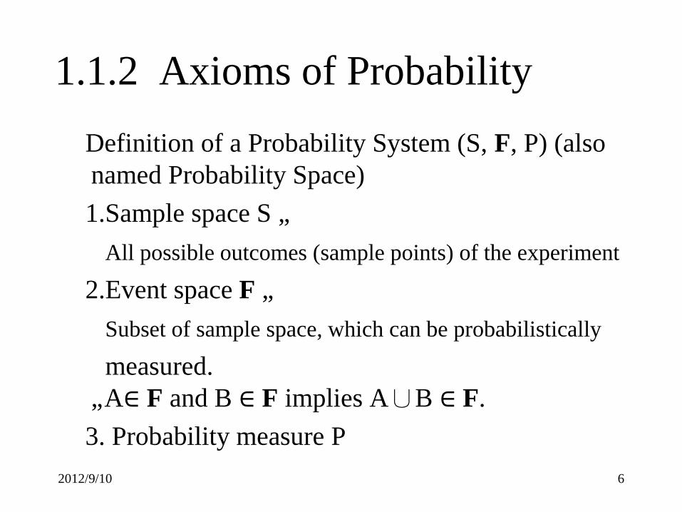
1.1.2 Axioms of Probability

Definition of a Probability System (S, F, P) (also

named Probability Space)

1.Sample space S „

All possible outcomes (sample points) of the experiment

2.Event space F „

Subset of sample space, which can be probabilistically

measured.

„ A∈ F and B ∈ F implies A∪B ∈ F.

3. Probability measure P

6 2012/9/10

1.1.2 Axioms of Probability

3. Probability measure P „

A probability measure satisfies:

† P(S) = 1 and P(EmptySet) = 0

For any A in F, 0 ≦ P(A) ≦ 1.

† For any two mutually exclusive events A

and B, P(A∪ B) = P(A) + P(B)

7 2012/9/10

1.1.2 Axioms of Probability

8 2012/9/10

1.1.3 Properties from Axioms

9 2012/9/10

1.1.4 Conditional Probability

10 2012/9/10

1.1.5 Random Variable

11 2012/9/10

1.1.5 Random Variable

12 2012/9/10

1.1.5 Random Variable

13 2012/9/10

1.1.5 Random Variable

14 2012/9/10

1.1.5 Random Variable

15 2012/9/10

1.1.6 Random Vector

16 2012/9/10

1.1.6 Random Vector

17 2012/9/10

1.1.6 Random Vector

18 2012/9/10

19

1.2 Mathematical Definition of a Random Process (RP)

The properties of RP

a. Function of time.

b. Random in the sense that before conducting an

experiment, not possible to define the waveform.

Sample space S function of time, X(t,s) (-T,T) mapping A random variable (r.v) is a real-valued function defined on the elements of the Sample space.

2012/9/10

20

(1.1)

2T:The total observation interval

(1.2)

= sample function λ←which is deterministic

At t = tk, the set{xj (tk) } constitutes a random

variable (RV).

To simplify the notation , let X(t,s) = X(t)

X(t):Random process, an ensemble of time functions

together with a probability rule.

Difference between RV and RP

RV: The outcome is mapped into a real number

RP: The outcome is mapped into a function of time

Tt-Tt,sX )( S

)(),( txstXs jjj

)(tx j

2012/9/10

21

Figure 1.1 An ensemble of sample functions:

Note:X(t1),X(t2)…X(tn) are statistically independent for any t1,t2 ,…, tn

},,2,1|)({ njtx j

2012/9/10

22

1.3 Stationary Process Stationary Process :

The statistical characterization of a process is independent of

the time at which observation of the process is initiated.

Nonstationary Process:

Not a stationary process (unstable phenomenon )

Consider X(t) which is initiated at t = ,

X(t1),X(t2)…,X(tk) denote the RV obtained at t1,t2…,tk

For the RP to be stationary in the strict sense (strictly stationary)

The joint distribution function independent of τ

(1.3)

For all time shift t, all k, and all possible choice of t1,t2…,tk

)...()..( ,)()(,,)(),...,( 11

11kk xxFxxF

kk t,...,XtXτtXτtX

2012/9/10

1.3 Random Process

23 2012/9/10

24

X(t) and Y(t) are jointly strictly stationary if the joint

finite-dimensional distribution of and

are invariant w.r.t. the origin t = 0.

Special cases of Eq.(1.3)

1. k = 1, for all t and t (1.4)

2. k = 2 , t = -t1

(1.5)

which only depends on t2-t1 (time difference)

)()( 1 ktXtX )()( 1 'tY'tY j

)(F)(F)(F )()( xxx XτtXtX

),(F),( 212 )((0),)(),( 121

21xxxxF ttXXtXtX

2012/9/10

1.3 Stationary

25 2012/9/10

26 2012/9/10

27 2012/9/10

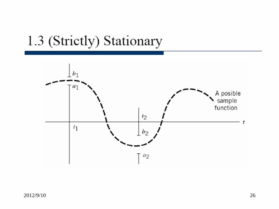
1.3 (Strictly) Stationary

Why introducing “stationarity”?

With stationarity, we can certain that the

observations made at different time

instances have the same distributions!

28 2012/9/10

29

1.4 Mean, Correlation,and Covariance Function Let X(t) be a strictly stationary RP

The mean of X(t) is

(1.6)

(indep. of t) for all t (1.7)

fX(t)(x) : the first order pdf which is independent of time.

The autocorrelation function of X(t) is

for all t1 and t2 (1.8)

is the second order pdf

)()( tXEtX

xxxf tX d )(

)(

)(

),(

),(

)()( )(R

12

-

-2121)((0)21

-

-2121)()(21

2121

12

21

ttR

dxdxxxfxx

dxdxxxfxx

tXtXE,tt

X

ttXX

tXtX

X

X

1 2( ) ( ) 1 2( , )X t X t

f x x

stationary

2012/9/10

30

The autocovariance function

(1.10)

Which is of function of time difference (t2-t1).

We can determine CX(t1,t2) if X and RX(t2-t1) are known.

Note that:

1. X and RX(t2-t1) only provide a partial description.

2. If X(t) = X and RX(t1,t2)=RX(t2-t1),

then X(t) is wide-sense stationary (stationary process).

3. The class of strictly stationary processes with finite

second-order moments is a subclass of the class of all

stationary processes.

4. The first- and second-order moments may not exist.

)(

)()( )(C

2

12

2121

XX

XXX

ttR

tXtXE,tt

2

1 1( . . ( ) , )

1e g f x x

x

2012/9/10

1.4 Wide-Sense Stationary (WSS)

31 2012/9/10

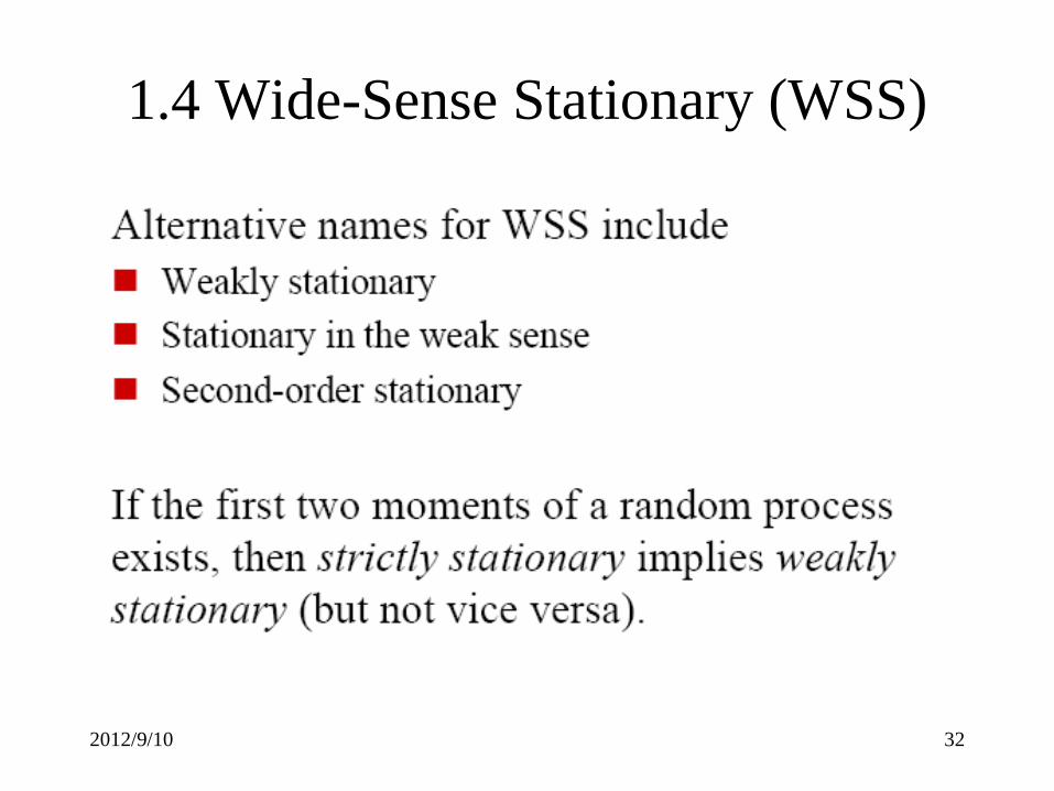
1.4 Wide-Sense Stationary (WSS)

32 2012/9/10

1.4 Cyclostationarity

33 2012/9/10

34

Properties of the autocorrelation function

For convenience of notation , we redefine

1. The mean-square value

2.

3.

( ) ( ) ( )R x t x tt t

(1.11) allfor , )()()( ttXτtXERX t

(1.12) 0 τ , )((0) 2 tXERX

(1.13) τ)()( RRX t

(1.14) (0))( XX RR t

( ) ( )x x t t t

( )R t

2012/9/10

35

0)]([)]()([2)]([ 22 tXEtXtXEtXE tt

0)(2)0(2 tXX RR

)0()()0( XXX RRR t

0)(2)]([2 2 tXRtXE

)0(|)(| XX RR t

Proof of property 3:

0]))()([( Consider 2 tXτtXE

2012/9/10

36

The RX(t) provides the interdependence information

of two random variables obtained from X(t) at times

t seconds apart

2012/9/10

37

Example 1.2 (1.15)

(1.16)

(1.17)

Θ)2cos()( tπfAtX c

elsewhere,0

,2

1

)(πθπ

πf

f

θπ π

( ) cos( )2

2

( ) ( ) 2X c

AR E X t τ X t πft t

2012/9/10

38

Appendix 2.1 Fourier Transform

2012/9/10

39

We refer to |G(f)| as the magnitude spectrum of the signal g(t),

and refer to arg {G(f)} as its phase spectrum.

2012/9/10

40

DIRAC DELTA FUNCTION

Strictly speaking, the theory of the Fourier transform is

applicable only to time functions that satisfy the Dirichlet

conditions. Such functions include energy signals. However,

it would be highly desirable to extend this theory in two

ways:

1. To combine the Fourier series and Fourier transform into a

unified theory, so that the Fourier series may be treated as a

special case of the Fourier transform.

2. To include power signals (i.e., signals for which the average

power is finite) in the list of signals to which we may apply

the Fourier transform.

2012/9/10

41

The Dirac delta function or just delta function, denoted by ,

is defined as having zero amplitude everywhere except

at , where it is infinitely large in such a way that it

contains unit area under its curve; that is

and

)(t

0t

,0)( t 0t

1)( dtt

)()()( 00 tgdttttg

)()()( tgdtg ttt

(A2.3)

(A2.4)

(A2.5)

(A2.6) 2012/9/10

42 2012/9/10

43 2012/9/10

44

Example 1.3 Random Binary Wave / Pulse

1. The pulses are represented by ±A volts (mean=0).

2. The first complete pulse starts at td.

3. During , the presence of +A

or –A is random.

4.When , Tk and Ti are not in the same pulse

interval, hence, X(tk) and X(ti) are independent.

elsewhere,0

0,1

)(Tt

Ttf ddTd

nTttTn d )1(

Ttt ik

0)()()()( ikik tXEtXEtXtXE

2012/9/10

45

Figure 1.6 Sample function of random binary wave.

2012/9/10

46

Solution 1 For

X(tk) and X(ti) occur in the same pulse interval

, , 0 , 0,ik i k k i

t t T t t t t

T-tt

-ttT- t

id

ikd

i.e.,

iff

TttT

ttA

dtT

A

dttftXtXE

ttTtAttXtXE

ik

ik

-ttT-

d

dd

-ttT-

Tik

ikd

dik

ik

ik

d

)(1

)(A)()(

elsewhere0,

--, )()(

2

0

2

0

2

2

2012/9/10

47

Similar reason for any other value of tk

What is the Fourier Transform of ?

Reference : A.Papoulis, Probability, Random

Variables and Stochastic Processes,

Mc Graw-Hill Inc.

)(tXR

where,

0,

),(1)(

2

ikX -ttτ

Tτ

TτT

τA

R

t

2 2( ) sin ( )x

S f A T c fT

2012/9/10

Solution 2

48 2012/9/10

49 2012/9/10

50 2012/9/10

51 2012/9/10

52 2012/9/10

53 2012/9/10

54 2012/9/10

55

Cross-correlation Function of X(t) and Y(t)

and

Note and are not general even

functions.

The correlation matrix is

If X(t) and Y(t) are jointly stationary

(1.20) )()()(

(1.19) )()()(

uXtYEt,uR

uYtXEt,uR

YX

XY

),( utRYX),( utRXY

),(),(

),(),(),(

utRutR

utRutRut

YYX

XYX

R

utτwhere

RR

RR

YYX

XYX

(1.21) )( )(

)( )()(

tt

tttR

( , ), ( , )x y

R t u R t u are autocorrelation functions

2012/9/10

56

(1.22) )(

)](()([

)]()([

)]()([ )(

,Let

τR

tXtYE

XYE

YXEτR

μτt

YX

XY

t

t

t

Proof of :

)]()( E[)( τtYtXτRXY

)()( τRR YXXY t

2012/9/10

X t

c c c

c c cX t

X c c

R E X t X t τ X t X t

E X t X t τ E πf t πf t πf τ

E X t X t τ πf t πf t πf τ d

R τ E πf t πf τ E

E E

t t

=

12 1 2 1 2( )

2

( )0

( ) ( ) ( ) ( ) ( )

( ) ( ) cos(2 )sin(2 2 )

1( ) ( )cos(2 )sin(2 2 )

2

1( ) sin(4 2 2 ) sin(

2 c

X c

πf τ .

R τ πf τ

( )2 ) 1 23

1( )sin(2 )

2

57

Example 1.4 Quadrature-Modulated Process

where X(t) is a stationary process and is uniformly

distributed over [0, 2].

),2(sin)()(

)2(cos)()(

2

1

tπftXtX

tπftXtX

c

c

12

1 2

At sin( ) 0, ( ) 0 ,

( ) and ( ) are orthogonal at some fixed t.

0, 2c

πf τ R

X t X t

t t

= 0

2012/9/10

58

1.5 Ergodic Processes

Ensemble averages of X(t) are averages “across the process”.

(in sample space)

Long-term averages (time averages) are averages “along the

process ” (in time domain)

DC value of X(t) (random variable)

If X(t) is stationary,

(1.24) )(2

1)(

T

Tx dttx

TTμ

(1.25)

2

1

)(2

1)(E

?

X

T

TX

T

Tx

μ

dt μT

dttxET

T μ

2012/9/10

59

represents an unbiased estimate of

The process X(t) is ergodic in the mean, if

The time-averaged autocorrelation function

If the following conditions hold, X(t) is ergodic in the

autocorrelation functions

0)(varlim b.

)(lim a.

T μ

μTμ

xT

XxT

)(TxX

variable.random a s ) (

)261()()(2

1)(

iT,R

. dt txτtxT

τ,TR

x

T

Tx

t

0)(varlim

)(),(lim

,TR

τRTR

xT

XxT

t

t

2012/9/10

60

Linear Time-Invariant Systems (stable)

a. The principle of superposition holds

b. The impulse response is defined as the response of the system with zero initial condition to a unit impulse or δ(t) applied to the input of the system

c. If the system is time invariant, then the impulse response function is the same no matter when the unit impulse is applied

d. The system can be characterized by the impulse response h(t)

e. The Fourier transform of h(t) is denoted as H(f)

2012/9/10

61

1.6 Transmission of a random Process Through a Linear Time-Invariant Filter (System)

where h(t) is the impulse response of the system

If E[X(t)] is finite

and system is stable

If X(t) is stationary,

H(0) :System DC response.

(f)=H(f)X(f)1 1 1( ) ( ) ( )

-Y t h τ X t τ dτ Y

(1.28) )()(

)()(

(1.27) )()(

)()(

111

111

111

-X

-

-

Y

dττtμτh

dττtxEτh

dττtXτhE

tYE tμ

(1.29) ),0( )( 11 Hμdττhμμ X

-XY

2012/9/10

62

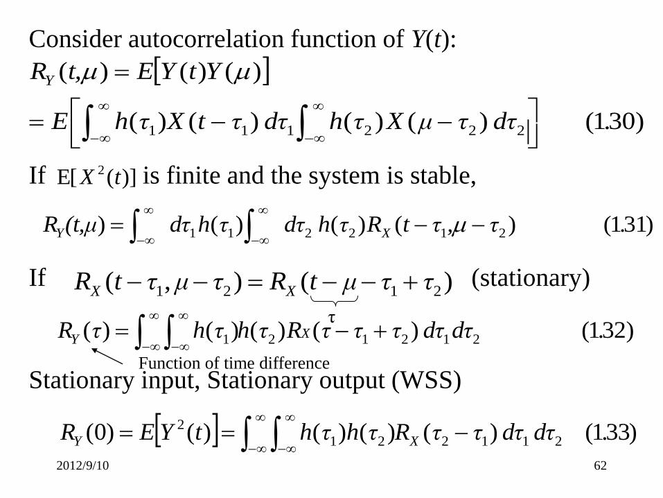
Consider autocorrelation function of Y(t):

If is finite and the system is stable,

If (stationary)

Stationary input, Stationary output (WSS)

)301( )()( )()(

)()()(

222111 . dττμXτhdττtXτhE

YtYEt,R

Y

)](E[ 2 tX

)311( )()( )( ) 212211 . τ,τtRτhdττhdτ(t,μR X

Y

)(),( 2121 ττμtRτμτtR XX

)321( )()()()( 212121 .dτdττττRτhτhτR X

Y

X

Y .dτdτττRτhτhtYER )331( )()()()()0( 211221

2

τ

Function of time difference

2012/9/10

63

1.7 Power Spectral Density (PSD)

Consider the Fourier transform of g(t),

Let H(f ) denote the frequency response,

Recall (1.30)

dfπftjfGtg

dtπftjtgfG

)2exp()()(

)2exp()()(

1 1

2

1 2 2 1 1 2

(1 34)( ) ( )exp( 2 )

( ) ( )exp( 2 ) ( ) ( )

( )

X

.h τ H f j πfτ df

E Y t H f j fτ df h τ R τ τ dτ dτ

df H f

2 2 2 1 1 1

2 2 2

(1 35)

(1 36)

( ) exp( 2 )

( ) exp( 2 ) ( )exp( 2 )

X

X

.

.

dτ h τ R (τ τ ) j fτ dτ

df H f dτ h(τ ) j fτ R j fτ d

t t

(complex conjugate response of the filter)( )*

H f

12 - ttt 1 1 1 2 2 2( ) ( ) ( ) ( ) ( ) ( )E Y t Y u E h X t d h X dt t t t t t

let 2 1

1 2

t t t

t t t

2012/9/10

64

: the magnitude response

Define: Power Spectral Density ( Fourier Transform of )

Recall

Let be the magnitude response of an ideal narrowband filter

D f : Filter Bandwidth

)371( )2exp())()(22 . dτfj(τRfHdftYE

-X

-t

)391( )()()(

)381( )2exp()()(

22 .dffSfHtYE

. dπfτRfS

-X

-XX

tt

)331( )()()()( 2 11221

2 .dτdτττRτhτhtYE X

- -

in W/Hz)( )(Δ2)(

,continuous is )( andΔ If

2

cXcX

Xc

fSff StYE

fSff

(1.40)

)( fH

)τR(

)( fH

ff,

ff,|f|H

f

f

c

c

D

D

2121

0

1)(

2012/9/10

65

Properties of The PSD

Einstein-Wiener-Khintchine relations:

is more useful than !

)431( )2exp()()(

)421( )2exp()()(

. df fjτSτR

. dfjτRfS

XX

XX

t

tt

)( fSX)(τRX

)()( τRfS XX

2012/9/10

66

.df fS

fSf

e.

.fS

τ udufujuR

dτfjτRfd. S

. f fS

fSftYE

t Xc.

. df fStXb. E

. dτRa. S

X

XX

X

X

XX

X

X

X

XX

p )481( )(

)()(

:pdfa withassociated be can PSDThe

)471( )(

, )2exp()(

)2exp()()(

)461( allfor 0)(

0)()Δ2()(

,stationary is)(If

)451( )()(

)441( )()0(

2

2

t

t

( ) ( )R Rt t

2012/9/10

67

Example 1.5 Sinusoidal Wave with Random Phase

2

2

( ) cos(2 ), ~ ( , )

( ) cos(2 )2

( ) ( )exp( 2 )

exp( 2 ) exp( 2 ) exp( 2 )4

c

X c

X X

c c

X t A f t U

AR f

S f R j f d

Aj f j f j f d

t t

t t t

t t t t

Appendix 2

2

( ) ( )4

, exp 2 ( ) ( )

c c

c c

Af f f f

j f f d f f

t

(Example 1.2)

The spectral Analyzer can not detected the phase, so the phase information is lost. 2012/9/10

68

Example 1.6 Random Binary Wave (Example 1.3)

Define the energy spectral density of a pulse as

(1.50) )(sincA

)2exp()1()(

0

)1()(

0if

1if ,

, )(

22

2

2

f TT

dfjT

AfS

T

TT

AR

m(t)

m(t)

A

AtX

T

TX

X

tt

t

t

ttt

(1.52) )(

)(S

(1.51) )(sinc)( 222

T

ff

f TTAfε

g

X

g

2012/9/10

69

Example 1.7 Mixing of a Random Process with a Sinusoidal Process

(1.55) )()(4

1

))(2exp())(2exp()(4

1

)2exp()( )(

(1.54) )2cos()(2

1

)224cos()2cos()(2

1

)2cos()22cos()()(

)()( )(

(1.53) )(0,2~ , )2cos()()(

cXcX

ccX

YY

cX

cccX

ccc

Y

c

ffSffS

dffjffjR

dfjRfS

fR

ftffER

tfftfEtXτtXE

tYτtYER

UtftXtY

tttt

ttt

tt

ttt

t

t

We shift the to the right by , shift it to the left by ,

add them and divide by 4.

)( fSX cf cf2012/9/10

70

Relation Among The PSD of The Input and Output Random Processes

Recall (1.32)

(1.32)

( )

, or

1 2 1 2 1 2

1 2 1 2 1 2

1 2 0 0 1 2

( ) ( ) ( ) ( )

( ) ( ) ( )exp( 2 )

( )

Y X

Y X

Y

R h h R d d

S f h h R j f d d d

Let

S f

t t t t t t t t

t t t t t t t t t

t t t t t t t t

( )

1 2 0 0 2 1 1 2 0

2

( ) ( ) ( )exp( 2 )exp( 2 )exp( 2 )

( ) ( ) * ( )

( )

X

X

X

h h R j f j f j f dτ dτ dτ

S f H f H f

H f S f

t t t t t t

(1.58)

h(t) X(t)

SX (f)

Y(t)

SY (f)

2012/9/10

71

Relation Among The PSD and

The Magnitude Spectrum of a Sample Function

Let x(t) be a sample function of a stationary and ergodic Process X(t).

In general, the condition for Fourier transformable is

This condition can never be satisfied by any stationary x(t) of infinite duration.

We may write

If x(t) is a power signal (finite average power)

Time-averaged autocorrelation periodogram function

(1.61) )()(2

1lim)(

average timeTake Ergodic

(1.60) )2exp()(),(

dttxtxT

R

dtftjtxTfX

T

TTX

T

T

tt

(1.59) )( dttx

(1.62) ),(2T

1 )()(

2

1 2

TfXdttxtxT

T

T

t

For fixed f, it is a r.v. (from one sample function to another) 2012/9/10

72

Take inverse Fourier Transform of right side of (1.62)

From (1.61),(1.63),we have

Note that for any given x(t) periodogram does not converge as

Since x(t) is ergodic

(1.67) is used to estimate the PSD of x(t)

(1.63) )2exp(),(2

1)()(

2

1 2df fTjTfX

Tdttxtx

T

Tt

(1.64) )2exp(),(2

1lim)(

2dffjTfX

TR

TX

tt

T

(1.66)

Recall (1.43) ( )

2

2

2

1( ) ( ) lim ( ) exp( 2 )

2

1( ) lim ( ) exp( 2 )

2

( )exp( 2 )

1( ) lim ( , )

2

X XT

XT

X X

XT

E R R E X f T j f dfT

R E X f T j f dfT

R S f j f df

S f E X f TT

t t t

t t

t t

(1.67)21

lim ( )exp( 2 )2

T

TTE x t j ft dt

T

2012/9/10

73

Cross-Spectral Densities

(1.72) )()()(

(1.22) )()(

)2exp()()(

)2exp()()(

real. benot may )( and )(

(1.69) )2exp()()(

(1.68) )2exp()()(

fSfSfS

τRτR

dfπfτjfSτR

dfπfτjfSτR

fSfS

dfjRfS

dfjRfS

YXYXXY

YXXY

YXYX

XYXY

YXXY

YXYX

XYXY

ttt

ttt

2012/9/10

74

Example 1.8 X(t) and Y(t) are uncorrelated and zero mean stationary processes.

Consider

Example 1.9 X(t) and Y(t) are jointly stationary.

(1.75) )()()(

)()()(

fSfSfS

tYtXtZ

YXZ

Let

( ) (1.77

11 1 1 2 2 2 2

1 1 2 2 1 2 1 2

1 1 2 2 1 2 1 2

( , ) ( ) ( )

( ) ( ) ( ) ( )

( ) ( ) ( , )

( ) ( ) ( )

VZ

XY

VZ XY

R t u E V t Z u

E h X t d h Y u d

h h R t u d d

τ t u

R h h R d d

t t t t t t

t t t t t t

t t t t t t t t

)

1 2( ) ( ) ( ) ( )XYVZ

F

S f H f H f S f

1 2 1 2t ut t t t t

2012/9/10

75

1.8 Gaussian Process

Define : Y as a linear functional of X(t) (泛函數)

The process X(t) is a Gaussian process if every linear

functional of X(t) is a Gaussian random variable

T

dttXtgY0

(1.79) )()(

(1.81) (0,1) as , )2

exp(2

1)( Normalized

(1.80) 2

)(exp

2

1)(

2

2

2

Ny

yf

yyf

Y

Y

Y

Y

Y

( g(t): some function and the integral exists)

( e.g g(t): (t) )

Fig. 1.13 Normalized Gaussian distribution 2012/9/10

76

Central Limit Theorem

Let Xi , i =1,2,3,….N be (a) statistically independent R.V.

and (b) have mean and variance .

Since they are independently and identically distributed (i.i.d.)

Normalized Xi

The Central Limit Theorem

The probability distribution of VN approaches N(0,1)

as N approaches infinity.

Note: For some random variables, the approximation is poor even N is quite large.

N

i

iN

i

i

Xi

X

i

YN

Y

Y

NiXY

1

1V Define

.1Var

,0 EHence,

1,2,...., )(1

Xμ

2

Xσ

2012/9/10

77

Properties of A Gaussian Process

1.

0

0

Define ( )

( )

where ( )

0

0

0

0

( ) ( ) ( )

( ) ( )

( ) ( )

( ) ( )

T

T

Y

T

Y

T

Y t h t X d

Z g t h t X τ d dt

g t h t dt X τ d

g X dτ

g g

t t t

t t

t t

t t

t

0

( )

By definition is a Gaussian random variable (1.81)

( ) is Gaussian0

( )

( ) ( ) , 0

Y

T

t h t dt

Z

Y t h t X d t

t

t t t

X(t) h(t)

Y(t)

Gaussian in Gaussian out

2012/9/10

78

2. If X(t) is Gaussisan

Then X(t1) , X(t2) , X(t3) , …., X(tn) are jointly Gaussian.

Let

and the set of covariance functions be

,....,n,itXE itX i21 )()(

X

x μ Σ x μ

μ

,

where

Then (1.85)

where mean vector

1

( ) ( )

1 2

1,( ),..., ( ) 1 1

2 2

1 2

( , ) ( ) ( ) 1 2

( ) ( ) ( )

1 1( ..., ) exp( ( ) ( ))

2(2 )

, ,.

k i

n

iX k i k X t X t

Tn

T

X t X t n n

C t t E X t X t k,i , ,...,n

X t ,X t ,....,X t

f x x

D

Σ

Σ

covariance matrix {

determinant of covariance matrix

, 1

...,

( , )}

T

n

n

X k i k iC t t

D

2012/9/10

Supplemental Material

2012/9/10 79

2012/9/10 80

2012/9/10 81

2012/9/10 82

2012/9/10 83

84

3. If a Gaussian process is stationary then it is strictly stationary.

(This follows from Property 2)

4. If X(t1),X(t2),…..,X(tn) are uncorrelated as

Then they are independent

Proof : uncorrelated

is also a diagonal matrix, Δ=determinant of Σ

(1.85)

.21, ]))(()([( where,

0

0

22

2

2

1

,n,itXEtXE iii

n

Σ

x μ Σ x μ

x

where ( ) and ( )

1

1,( ), , ( ) 1 1

2 2

1

2

2

1 1( ..., ) exp( ( ))

2(2 )

( ) ( )

1exp

22

n

i

i

i

T

X t X t n n

n

X X i

i

i X

i i X i

ii

f x x

f f x Independent

xX X t f x

D

0)])()()([( )()( ik tXitXk tXtXE

1Σ

2012/9/10

85

1.9 Noise

· Shot noise

· Thermal noise

k: Boltzmann’s constant = 1.38 x 10-23 joules/K, T is the

absolute temperature in degree Kelvin.

22

2

2

22

amps 41

41

volts 4

fkTGfR

kTVER

IE

fkTRVE

TNTN

TN

DD

D

2012/9/10

86

· White noise

(1.93)

(1.94)

:equivalent noise temperature of the receiver

( ) (1.95)2

0

0

0

0

( )2

( )

( ) ( )exp( 2 )2

( )

W

e

e

W

W w

NS f

N kT

T

NR

NS f R j f d

f t

t t

t t t

1 Table A6.31, ( )f f δ δ 2012/9/10

87

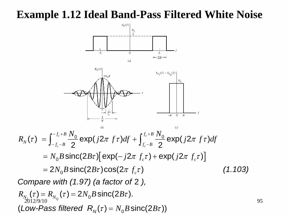
Example 1.10 Ideal Low-Pass Filtered White Noise

)2sinc(

(1.97) )2exp(2

)(

(1.96)

02)(

0

0

0

t

tt

BBN

df fjN

R

B f

B f-B N

fS

B

BN

N

2012/9/10

88

Example 1.11 Correlation of White Noise with a Sinusoidal Wave

White noise

2

(1.98)

The variance of is

0

1 1 2 2 1 20 0

1 2 1 20

2'( ) ( )cos(2 )

( )

2( )cos(2 ) ( )cos(2 )

2( ) ( ) cos(2 )cos(2 )

T

c

T T

c c

c c

w t w t f t dtT

w' t

E w t f t w t f t dt dtT

E w t w t f t f tT

2

From (1.95)

1 20

1 2 1 2 1 20 0

01 2 1 2 1 2

0 0

20 0

0

2( , )cos(2 )cos(2 )

2( )cos(2 )cos(2 )

2

cos (2 )2

T T

T T

W c c

T T

c c

T

c

dt dt

R t t f t f t dt dtT

Nt t f t f t dt dt

T

N N f t dt

T

(1.99)

X T

dt0

integer is , , )2cos(2

kT

kftf

Tcc

)(tw )(' Tw

)(' Tw

)(' Tw

2012/9/10

89

1.10 Narrowband Noise (NBN)

Two representations

a. in-phase and quadrature components (cos(2 fct) ,sin(2 fct))

b.envelope and phase

1.11 In-phase and quadrature representation

signals pass-low are )( and )(

(1.100) )2sin()()2cos()()(

tntn

t ftnt ftntn

Q

Q

I

ccI

(sample function)

0( )

T

dt2012/9/10

90

Important Properties

1.nI(t) and nQ(t) have zero mean.

2.If n(t) is Gaussian then nI(t) and nQ(t) are jointly Gaussian.

3.If n(t) is stationary then nI(t) and nQ(t) are jointly stationary.

4.

5. nI(t) and nQ(t) have the same variance .

6.Cross-spectral density is purely imaginary. (problem 1.28)

7.If n(t) is Gaussian, its PSD is symmetric about fc, then nI(t) and nQ(t)

are statistically independent. (problem 1.29)

(1.101) otherwise

0

, )()()()(

Bf-BffSffSfSfS

cNcN

NN QI

2

0N

(1.102)

otherwise

0

,

)( )(

Bf-BffSffSj

fSfS

cNcN

NNNN IQQI

2012/9/10

1.

From figure 1.19(a), we see that

Proof of e.q. (1.101)

Supplement

2012/9/10 91

2012/9/10 92

2.

From figure 1.19(a), we see that

Supplement

2012/9/10 93

2012/9/10 94

95

Example 1.12 Ideal Band-Pass Filtered White Noise

(1.103)

Compare with (

0 0

0

0

( ) exp( 2 ) exp( 2 )2 2

sinc(2 ) exp( 2 ) exp( 2 )

2 sinc(2 )cos(2 )

c c

c c

f B f B

Nf B f B

c c

c

N NR j f df j f df

N B B j f j f

N B B f

t t t

t t t

t t

N

1.97) (a factor of ),

Low-Pass filtered R

0

0

2

( ) ( ) 2 sinc(2 ).

( ( ) sinc(2 ))

I QN NR R N B B

N B B

t t t

t t

2012/9/10

96

1.12 Representation in Terms of Envelope and Phase Components

Let NI and NQ be R.V.s obtained (at some fixed time) from nI(t)

and nQ(t). NI and NQ are independent Gaussian with zero mean and

variance .

(1.107) )(

)(tan)(

Phase

(1.106) )()()(

Envelope

(1.105) )(2cos)()(

1

21

22

tn

tnt

tntntr

ttftrtn

I

Q

QI

c

22012/9/10

97

(1.108) )2

exp(2

1),(

2

22

2,

QI

QINN

nnnnf

QI

(1.112)

(1.111) sin

(1.110) cosLet

(1.109) )2

exp(2

1),(

2

22

2

,

r dr dψ dndn

ψrn

ψrn

dn dnnn

dndnnnf

QI

Q

I

QI

QI

QIQINNQI

2012/9/10

98

Substituting (1.110) - (1.112) into (1.109)

(1.113)

0 20 2

el

, ,

2

2 2

2

, 2 2

( , ) ( , )

exp( )2 2

( , ) exp( )2 2

1

, ( ) 2

0

I QN N I Q I Q R Ψ

R Ψ

Ψ

f n n dn dn f r rdrd

r rdrd

r rf r

f

(1.114)

sewhere

(1.115)

elsewhere

( ) is Rayleigh distribution.

For convenienc

2

2 2exp( ) , 0

( ) 2

0

R

R

r rr

f r

f r

e , let . ( ) ( ) (Normalized)

, ( ) (1.118)

elsewhere

2

exp( ) 02

0

V R

V

rν f ν f r

σ

f ν

2012/9/10

99

Figure 1.22 Normalized Rayleigh distribution.

2012/9/10

100

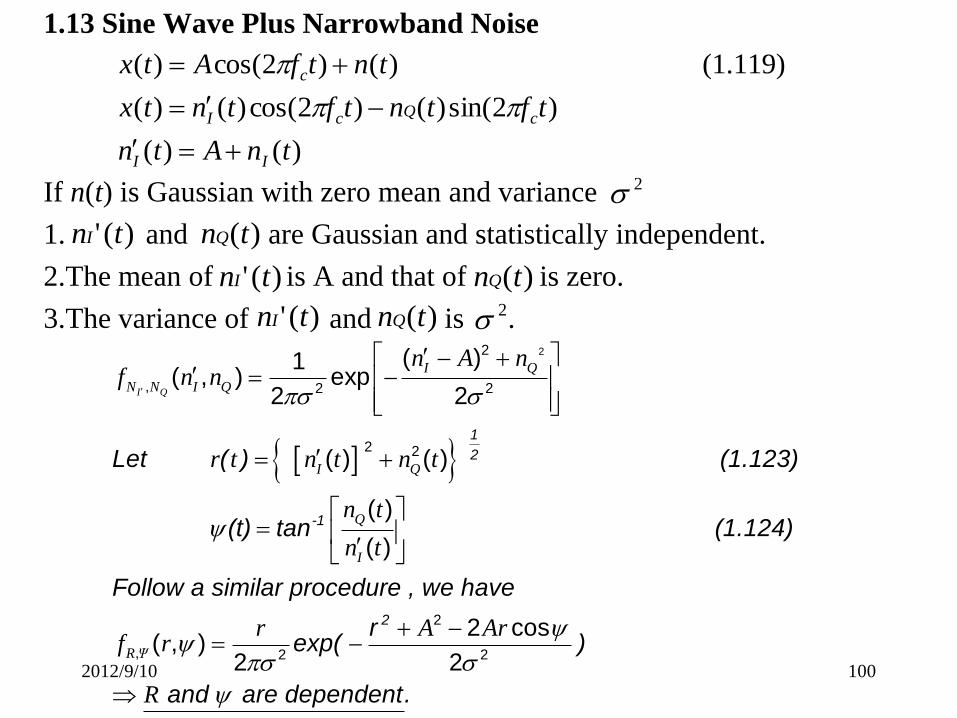
1.13 Sine Wave Plus Narrowband Noise

If n(t) is Gaussian with zero mean and variance

1. and are Gaussian and statistically independent.

2.The mean of is A and that of is zero.

3.The variance of and is .

)()(

)2sin()()2cos()()(

(1.119) )()2cos()(

tnAtn

tftntftntx

tntfAtx

II

cQcI

c

1

2

-1

Let ( ) (1.123)

(t) tan

22

, 2 2

2 2

( )1( , ) exp

2 2

( ) ( )

( )

( )

I Q

I Q

N N I Q

I Q

Q

I

n A nf n n

r t n t n t

n t

n t

2

(1.124)

Follow a similar procedure , we have

rexp( )

and are dependent.

2

, 2 2

2 cos( , )

2 2R Ψ

r A Arf r

R

2

2

)(' tnI )(tnQ

)(' tnI )(tnQ

)(' tnI )(tnQ

2012/9/10

101

The modified Bessel function of the first kind of zero

order is defined as (Appendix 3)

It is called Rician distribution.

If

2

0 22

22

2

2

0 ,

(1.126) )dcosexp()2

exp(2

),( )(

ArArr

drfrf ΨRR

(1.127)

Let (1.128)

2

00

2 2

02 2 2 2

1( ) exp( cos )

2

exp( ) ( )2

R

I x x d

Ar r r A Arx , f (r) I

σ

=1,

2

00

10, (0)

2A I d

it is Rayleigh distribution. 2012/9/10

102

(1.132) )()2

exp(

(1.131) )( )(

,

0

22

avIav

v

rfvf

Aa

rNormalized

RV

Figure 1.23 Normalized Rician distribution. 2012/9/10