chapter 1 - problem solutions - li group 李巨...
TRANSCRIPT

CHAPTER 1 - PROBLEM SOLUTIONS A. PROFICIENCY PROBLEMS 1. The plot below of load vs. extension was obtained using a specimen (shown in the following figure)
of an alloy remarkably similar to the aluminum-killed steel found in automotive fenders, hoods, etc. The crosshead speed, v, was 3.3x10⁻⁴ inch/second. The extension was measured using a 2" extensometer as shown (G). Eight points on the plastic part of the curve have been digitized for you. Use these points to help answer the following questions.
Loa
d, p
ound
s
0.80.70.60.50.40.30.20.1
100
200
300
400
500
600
700
800
900
G = 2.0"
0.03"
0.5"
(0.0018, 405 )
(0.004, 458)
(0.10, 630 )
(0.20, 699)
(0.30, 729)
(0.40, 741.5 )
(0.50, 745 )
(0.80, 440 )
Extension, inches
D = 3.3 "
a. Determine the following quantities. Do not neglect to include proper units in your answer.
Yield stress Young's Modulus Ultimate tensile strength Total elongation Uniform elongation Post-uniform elongation Engineering strain rate
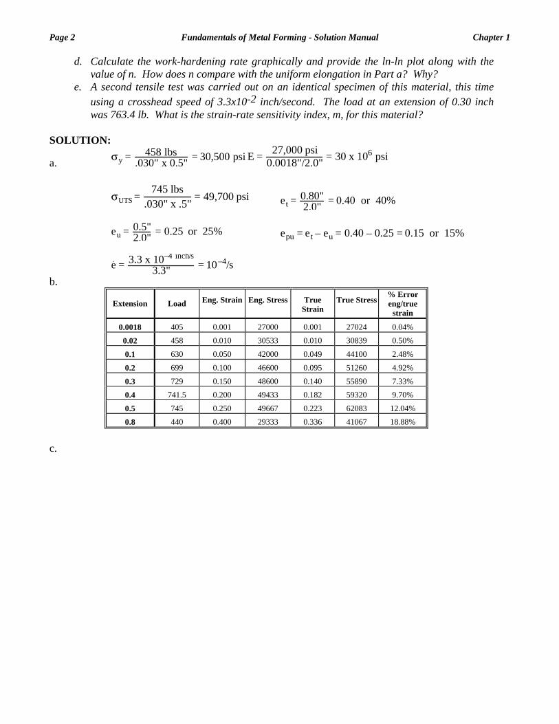
b. Construct a table with the following headings, left-to-right: Extension, load, engineering
strain, engineering stress, true strain, true stress. Fill in for the eight points on graph. What is the percentage difference between true and engineering strains for the first point?
(i.e., % = ______ x 100) What is the percentage difference between true and engineering strains for the last point? c. Plot the engineering and true stress-strain curves on a single graph using the same units.
Page 2 Fundamentals of Metal Forming - Solution Manual Chapter 1
d. Calculate the work-hardening rate graphically and provide the ln-ln plot along with the value of n. How does n compare with the uniform elongation in Part a? Why?
e. A second tensile test was carried out on an identical specimen of this material, this time using a crosshead speed of 3.3x10⁻² inch/second. The load at an extension of 0.30 inch was 763.4 lb. What is the strain-rate sensitivity index, m, for this material?
SOLUTION:
a. σy = 458 lbs
.030" x 0.5" = 30,500 psi E = 27,000 psi0.0018"/2.0" = 30 x 106 psi
σUTS =
745 lbs.030" x .5"
= 49,700 psi et = 0.80"
2.0" = 0.40 or 40%
eu = 0.5"
2.0" = 0.25 or 25% epu = et – eu = 0.40 – 0.25 = 0.15 or 15%
e = 3.3 x 10⁻⁴ inch/s
3.3" = 10–4/s b.
Extension Load Eng. Strain Eng. Stress True Strain
True Stress% Error eng/true
strain
0.0018 405 0.001 27000 0.001 27024 0.04%
0.02 458 0.010 30533 0.010 30839 0.50%
0.1 630 0.050 42000 0.049 44100 2.48%
0.2 699 0.100 46600 0.095 51260 4.92%
0.3 729 0.150 48600 0.140 55890 7.33%
0.4 741.5 0.200 49433 0.182 59320 9.70%
0.5 745 0.250 49667 0.223 62083 12.04%
0.8 440 0.400 29333 0.336 41067 18.88%
c.
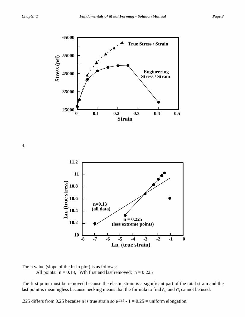
Chapter 1 Fundamentals of Metal Forming - Solution Manual Page 3
25000
35000
45000
55000
65000
0 0.1 0.2 0.3 0.4 0.5
Stre
ss (p
si)
Strain
True Stress / Strain
EngineeringStress / Strain
d.
10
10.2
10.4
10.6
10.8
11
11.2
-8 -7 -6 -5 -4 -3 -2 -1 0
Ln.
(tru
e st
ress
)
Ln. (true strain)
n=0.13 (all data)
n = 0.225 (less extreme points)
The n value (slope of the ln-ln plot) is as follows: All points: n = 0.13, Wth first and last removed: n = 0.225 The first point must be removed because the elastic strain is a significant part of the total strain and the last point is meaningless because necking means that the formula to find εt, and σt cannot be used. .225 differs from 0.25 because n is true strain so e.225 - 1 = 0.25 = uniform elongation.

Page 4 Fundamentals of Metal Forming - Solution Manual Chapter 1
e.
m =
ln p2/p1ln v2/v1
=ln 763.4 lb
729 lb
ln 3.3 x 10⁻²/s3.3 x 10–4 /s
= ln 1.047ln 100 = .046
4.605 = 0.010
2. Starting from the basic idea that tensile necking begins at the maximum load point, find the true
strain and engineering strain where necking begins for the following material laws. Derive a general expression for the form and find the actual strains.
a. (Swift)σ = k (ε + εo)n σ = 500 (ε + 0.05)0.25 1
b. (Ludwik) σ = σo + k (ε + εo)n σ = 100 + 500 (ε + 0.05)0.25
c. σ = σo (1 - Ae
-Bε) σ = 500 1 - 0.6 exp (-3ε) (Voce)2
d. σ = σo σ = 500 (Ideal) e. σ = σo + kε σ = 250 + 350 ε (Linear) f. (Trig) σ = k sin (Bε) σ = 500 sin (2πε)
SOLUTION: a. σ = k (ε + εo)n
dσ
dε = nk (ε + εo)n–1 = k(ε + εo)n = σ
n = εu + εo, εu = n – εo
for εo = 0.05, n = 0.25 εu = 0.20
b. σ = σo + k(ε + εo)
n
dσ
dε= nk (ε + εo)
n–1 = σo + k(ε + εo)n = σ
σo + k(ε + εo)n–1 ε + εo–n = 0
This is transcendental, so it cannot be solved algebraically. Let's solve it numerically by Newton's Method for the special case n = 0.25, εo = 0.05, σo = 100, k = 500.
1 H. W. Swift: Plastic Instability Under Plane Stress, J. Mech. Phys. Solids, 1952, Vol. 1, p.1. 2 E. Voce: The Relationship Between Stress and Strain For Homogeneous Deformation, J. Inst. Met: 1948, Vol. 74, p. 537-562, 760. E. Voce: The Engineer: 1953, Vol. 195, p.23. E. Voce: Metallurga: 1953, Vol. 51, p. 219.

Chapter 1 Fundamentals of Metal Forming - Solution Manual Page 5
F(ε) = σo + k(ε + εo)
n–1 ε + εo–n = 0
F′(ε) = k(n–2)(ε + εo)n–2 ε + εo–n + k(ε + εo)
n–1
Start from a trial of eu = 0.20 (from Part b)
Step (i) εu(i) F[εu(i)] F'[εu(i)] εu(i+1)
0 0.20 100 1,414 0.129
1 0.129 -29 3,078 0.138
2 0.138 -8.5 2,762 0.142 So, eu ≈ 0.142
c. σ = σo(1–Ae–Bε)
dσ
dε= BAσoe
–Bε = σo(1–Ae–Bε) = σ
BX = 1-X where X = Ae-Bε
X =
11+B
or ln X = ln1
1+B, ln A – Bε = ln
11+B,
–Bε = ln1
1+B– ln A
εu = –
1B
ln A – ln1
1+B=
1B
ln A(1+B)
for A = 0.6 B = 3: εu =
13
ln 0.6(4) = 0.29
d. , σ = σo
dσdε
= 0 = σo = σ (Never stable for constant σ . o
εu = 0 )
e. , σ = σo + kε dσ
dε= k = σo + kε = σ
, ε =
k–σo
k
for σo = 250, k = 350, εu =
350–250350
= 0.29
f. σ = k sin Bε
dσ
dε= kB cos Bε = k sin Bε
, , B = tan Bεε =
1B
tan–1 B
Page 6 Fundamentals of Metal Forming - Solution Manual Chapter 1
for , B = 2π, k = 500 ε =
12π
tan–1 2π = 0.22
3. What effect does a multiplicative strength coefficient (for example k in the Hollomon Law, k in
Problem 2.a., or σo in Problem 2.c.) have on the uniform elongation? SOLUTION: No effect. Because it is only the ratio of strength in one part of the tensile test (i.e. in the neck) to
another (outside the neck), multiplication of σ has no effect on stability. 4. For each of the explicit hardening laws presented in Problem 2, calculate the true stress at ε =
0.05, 0.10, 0.15, 0.20, 0.25 and plot the results on a (ln σ-ln ε) figure. Use the figure to calculate a best-fit n value for each material and compare this with the uniform strain calculated in Problem 2. Why are they different, in view of Eq. 1.16?
5. For each of the explicit hardening laws presented in Problem 2, plot the engineering stress-strain
curves and determine the maximum load point graphically. How do the results from this procedure compare with those obtained in Problems 2 and 4?
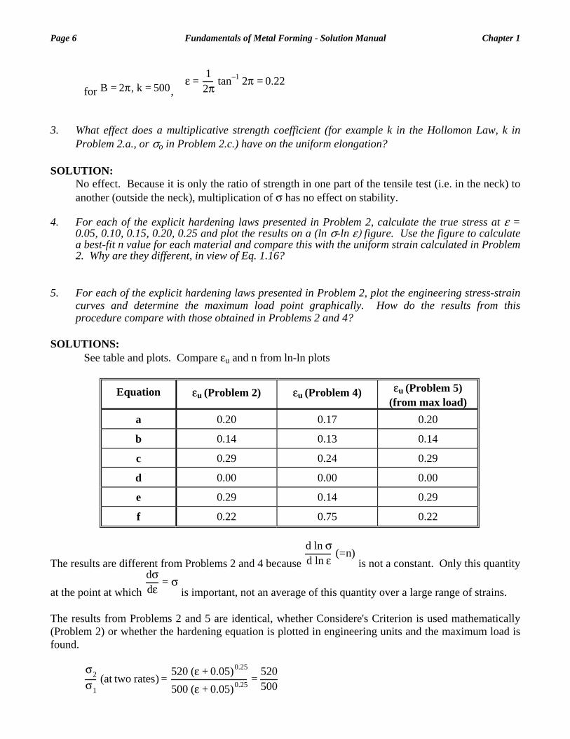
SOLUTIONS: See table and plots. Compare εu and n from ln-ln plots
Equation εu (Problem 2) εu (Problem 4) εu (Problem 5) (from max load)
a 0.20 0.17 0.20
b 0.14 0.13 0.14
c 0.29 0.24 0.29
d 0.00 0.00 0.00
e 0.29 0.14 0.29
f 0.22 0.75 0.22
The results are different from Problems 2 and 4 because d ln σd ln ε
(=n) is not a constant. Only this quantity
at the point at which dσ
dε= σ
impor
he results from Problems 2 and 5 are identical, whether Considere's Criterion is used mathematically
is tant, not an average of this quantity over a large range of strains. T(Problem 2) or whether the hardening equation is plotted in engineering units and the maximum load is found.
σ2σ1
(at two rates) =520 (ε + 0.05)0.25
500 (ε + 0.05)0.25 =520500

Chapter 1 Fundamentals of Metal Forming - Solution Manual Page 7
Problem 1-4 Stress Stress Stress Stress Stress Stress
Strain Part a Part b Part c Part d Part e Part f 0.05 281 381 268 155 242 500 0.1 311 411 278 500 285 294
0.15 334 434 309 500 303 405 0.2 354 454 335 500 320 476
0.25 370 470 358 500 338 500
ln stre ln stre ln stre ln stre ln stre ln stress ss ss ss ss ss ln strain Part a Part b Part c Part d Part e Part f -2.996 5.639 5.943 5.488 6.215 5.589 5.040 -2.303 5.740 6.019 5.627 6.215 5.652 5.683 -1.897 5.812 6.074 5.732 6.215 5.712 6.003 -1.609 5.868 6.117 5.815 6.215 5.768 6.164 -1.386 5.914 6.153 5.881 6.215 5.822 6.215
slope (n) 0.17 0.13 0.24 0.00 0.14 0.75
(Figure for Problem 1-4 follows.)
5
5.2
5.4
5.6
5.8
6
6.2
6.4
-3 -2.5 -2 -1.5 -1
abcdef
ln (t
rue
stre
ss)
ln (true strain)
d b
d
ae
c
f

Page 8 Fundamentals of Metal Forming - Solution Manual Chapter 1
0
100
200
300
400
500
0 0.1 0.2 0.3 0.4 0.5
abcdef
engi
neer
ing
stre
ss
engineering strain
Figure for Problem 1-4 (upper), for Problem 1-5 (lower).
Problem 1-5
True Eng. Eng. Stress Eng. Stress Eng. Stress Eng. Stress Eng. Stress Eng. Stress Strain Strain Part a Part b Part c Part d Part e Part f 0.01 0.01 245.0 344.0 206.8 495.0 251.0 31.1 0.02 0.02 252.1 350.1 213.2 490.1 251.9 61.4 0.03 0.03 258.1 355.1 219.1 485.2 252.8 90.9 0.04 0.04 263.1 359.2 224.8 480.4 253.6 119.5 0.05 0.05 267.5 362.6 230.0 475.6 254.5 147.0 0.06 0.06 271.2 365.4 234.9 470.9 255.2 173.3 0.07 0.07 274.4 367.6 239.5 466.2 255.9 198.5 0.08 0.08 277.1 369.5 243.7 461.6 256.6 222.4 0.09 0.09 279.5 370.9 247.7 457.0 257.3 244.9 0.1 0.11 281.6 372.0 251.3 452.4 257.9 265.9
0.11 0.12 283.3 372.9 254.7 447.9 258.4 285.5 0.12 0.13 284.8 373.4 257.8 443.5 259.0 303.6 0.13 0.14 286.0 373.8 260.7 439.0 259.5 320.1 0.14 0.15 287.0 373.9 263.3 434.7 259.9 334.9 0.15 0.16 287.8 373.9 265.7 430.4 260.4 348.2 0.16 0.17 288.4 373.6 267.9 426.1 260.8 359.7 0.17 0.19 288.9 373.3 269.8 421.8 261.1 369.7 0.18 0.20 289.2 372.7 271.6 417.6 261.4 377.9 0.19 0.21 289.4 372.1 273.2 413.5 261.7 384.4 0.2 0.22 289.5 371.3 274.6 409.4 262.0 389.3

Chapter 1 Fundamentals of Metal Forming - Solution Manual Page 9
0.21 0.23 289.4 370.5 275.8 405.3 262.2 392.6 0.22 0.25 289.2 369.5 276.8 401.3 262.4 394.2 0.23 0.26 289.0 368.4 277.7 397.3 262.6 394.1 0.24 0.27 288.6 367.3 278.4 393.3 262.7 392.5 0.25 0.28 288.2 366.1 279.0 389.4 262.8 389.4 0.26 0.30 287.7 364.8 279.5 385.5 262.9 384.8 0.27 0.31 287.1 363.4 279.8 381.7 263.0 378.7 0.28 0.32 286.4 362.0 280.0 377.9 263.0 371.2 0.29 0.34 285.7 360.5 280.1 374.1 263.0 362.4 0.3 0.35 284.9 359.0 280.1 370.4 263.0 352.3
0.31 0.36 284.1 357.4 279.9 366.7 262.9 341.0 0.32 0.38 283.2 355.8 279.7 363.1 262.9 328.5 0.33 0.39 282.2 354.1 279.3 359.5 262.8 315.0 0.34 0.40 281.2 352.4 278.9 355.9 262.6 300.5 0.35 0.42 280.2 350.7 278.4 352.3 262.5 285.1 0.36 0.43 279.1 348.9 277.8 348.8 262.3 268.8
Uniform strain (eng.) 0.22 0.15 0.34 0.00 0.33 0.25 Uniform Strain (true) 0.20 0.14 0.29 0.00 0.29 0.22
6. Tensile tests at two crosshead speeds (1mm/sec and 10mm/sec) can be fit to the following
hardening laws: at V1 = 1mm/sec, σ = 500 (ε + 0.05)0.25 at V2 = 10mm/sec, σ = 520 (ε + 0.05)0.25
What is the strain-rate sensitivity index for these two materials? Does it vary with strain? What is the uniform strain of each, according to the Considere Criterion?
SOLUTION:
m =
ln σ 2/σ 1
ln v2/v1
=ln 520/500
ln 10/1= 0.017
The strain-rate sensitivity is independent of strain because the ratio of stresses at the two strain rates is independent of strain. Substituting into the result for Problem 2a gives the uniform true strain in each case: εu (v2) = εu (v1) = n – εo = .25 – 0.05 = 0.20 7. Repeat Problem 6 with two other stress-strain curves: at V1 = 1mm/sec, σ = 550 ε0.25 at V2 = 10mm/sec, σ = 500 ε0.20
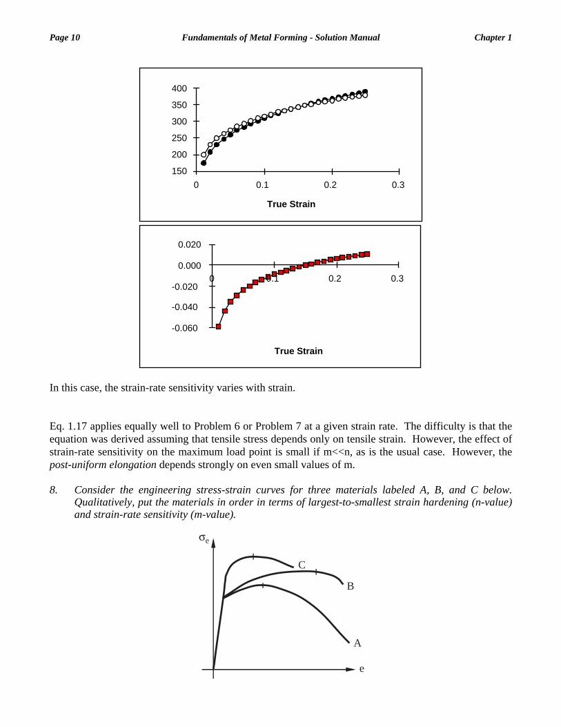
Plot the stress-strain curves and find the strain-rate sensitivity index at strains of 0.05, 0.15, and 0.25. In view of these results, does Eq. 1.17 apply to this material?
SOLUTION:
σ2σ1
=550 ε0.25
500 ε0.20 = 1.1 ε0.05
,
m =
ln 1.1 ε0.05
ln 10=
0.095 + 0.05 ln ε2.303
= 0.041 + 0.022 ln ε
Page 10 Fundamentals of Metal Forming - Solution Manual Chapter 1
True Strain
150
200
250
300
350
400
0 0.1 0.2 0.3
True Strain
-0.060
-0.040
-0.020
0.000
0.020
0 0.1 0.2 0.3
In this case, the strain-rate sensitivity varies with strain. Eq. 1.17 applies equally well to Problem 6 or Problem 7 at a given strain rate. The difficulty is that the equation was derived assuming that tensile stress depends only on tensile strain. However, the effect of strain-rate sensitivity on the maximum load point is small if m<<n, as is the usual case. However, the post-uniform elongation depends strongly on even small values of m. 8. Consider the engineering stress-strain curves for three materials labeled A, B, and C below.
Qualitatively, put the materials in order in terms of largest-to-smallest strain hardening (n-value) and strain-rate sensitivity (m-value).
σe
A
e
C
B

Chapter 1 Fundamentals of Metal Forming - Solution Manual Page 11
SOLUTION: Strain hardening (based on strain to maximum load) order: B, A, C. Strain-rate sensitivity (based on post-uniform strain) order: A, C, B. Ductility or formability (based on total strain to failure) order: A, B, C. 9. It is very difficult to match tensile specimens
precisely. For sheet materials, the thickness, width, and strength may vary to cause a combined uncertainty of about ±1% in stress. Considering this uncertainty of K's in Problem 6, calculate the range of m values which one might obtain if one conducted the tests at both rates several times.
σe
e
B
A
σe=315 MPa
σe=300 MPav1 = 10-3 m/s
v2 = 10-2 m/s
SOLUTION: From Problem 6, we recall that
m =
ln 520500
ln 10= 0.017
, but now we consider the range: 520 ± 1% x 520 = 515 to 525
and 500 ± 1% x 500 = 495 to 505
So, the combined uncertainty of m is in the range:
mlow =ln 515
505
ln 10= 0.009
mhigh =ln 525
495ln 10 = 0.026
= 0.017 ± 0.009
So, a ± 1% uncertainty in stress corresponds to a 50% uncertainty in m! ± 10. Considering the specimen-to-specimen variation mentioned in Problem 9, it would be very
desirable to test strain-rate sensitivity using a single specimen. Typically, "jump-rate tests" are conducted by abruptly changing the crosshead velocity during the test. Find the strain-rate sensitivity for the idealized result shown:
SOLUTION:
m =
ln 315300
ln 10= 0.021
11. In fact, the procedure outlined in Problem 10, while being convenient and attractive, has its own
difficulties. In order to obtain sufficient resolution of stress, it is necessary to expand the range and to move the zero point. Some equipment does not have this capability. More importantly, the response shown in Problem 10 is not usual. For the two more realistic jump-rate tests reproduced

Page 12 Fundamentals of Metal Forming - Solution Manual Chapter 1
below, find m values using the various points marked.
σe
e
B
A
v1 extrapolated
A=300 MPa
D
C
B=315 MPaC=330 MPaD=345 MPa
σe
e
B
A
A=315 MPaD
C
B=310 MPaC=300 MPaD=290 MPa
v2 extrapolated
v2 = 10-2 m/s
v2 = 10-2 m/s
v1 = 10-3 m/s
v1 = 10-3 m/s
OLUTION:
For the "up jump" in rate:
S
mB =
ln 315300
ln 10= 0.021
,
mC =
ln 330300
ln 10= 0.041
, mD =
ln 345300
ln 10= 0.061
For the "down jump" in rate:
mB =ln 310
315
ln 110
= 0.007,
mC =
ln 300315
ln 110
= 0.021,
mD =ln 290
315
ln 110
= 0.036
It should be apparent that neither the jump or continuous method eliminates the uncertainties.
. DEPTH PROBLEMS
2. If a tensile test specimen were not exactly uniform in cross section, for example if there were
B 1

Chapter 1 Fundamentals of Metal Forming - Solution Manual Page 13
initial tapers as shown below, how would you expect the measured true stress-strain curves to appear relative to one generated from a uniform specimen? Sketch the stress-strain curves you would expect.
(a) Uniform gage length
G
(b) General notch
������������
������������
���������
���������
(c) Severe notch
������������
������������
OLUTION:
he presence of a notch tends to concentrate the strain in the reduced gage section such that work
S Thardening occurs there rapidly. In a more severe notch, the stress state begins to have a lateral component (tending toward plane strain) which leads to more hardening. Therefore, one might expect the behavior to appear as shown.
UniformMild NotchSevere Notch
Engineering Strain
Eng
inee
ring
Str
ess
3. What is the relevance of the 0.2% offset in determining the engineering yield stress?
OLUTION: convenient number; small enough so that little strain hardening takes place but large
1 SIt is simply a

Page 14 Fundamentals of Metal Forming - Solution Manual Chapter 1
4. Some low-cost steels exhibit tensile stress-strain curves as shown below. What would you expect
enough to resolve using most tensile testing equipment. 1
to happen with regard to necking?
σe
e
OLUTION:
t, flat stage one should expect localization to begin. In fact, this happens in a narrow
5. It has been proposed that some materials follow a tensile constitutive equation which has additive
SDuring the firsband called a Luder's band, but as the strain there increases the material in the bank increases and the flow stress exceeds that of the surrounding material. The bank thus moves outward until the entire specimen is strained beyond the flat region. After that, straining takes place normally. 1
effects of strain hardening and strain-rate hardening rather than multiplicative ones:
multiplicative: σ = F(ε) G(ε)
additive: σ = F(ε) + G(ε)
In the first case one investigates
at constant ε by examining σ (V2)σ (V1)G(ε) , as we have done so far.
tch
In the second case, one would wa (V2) - σ (V1). Assume that an additive law of the following type were followed by a material:
σ = 500 ε
σ
0.25 + 25 εεo
0.030
where
εo is the base strain-rate where the strain hardening law is determined (i.e. a tensile test conducted at a strain rate of εo exhibits σ = 500ε0.25).
a. Given this law, determine the usual multiplicative m value at various strains from two
tensile tests, one conducted at εo and one at 10εo .
. Compare tensile results extracted from the additive law provided and the multiplicative
bone determined in Part a. [Use the m value obtained from the center of the strain range, at ε = 0.125.]
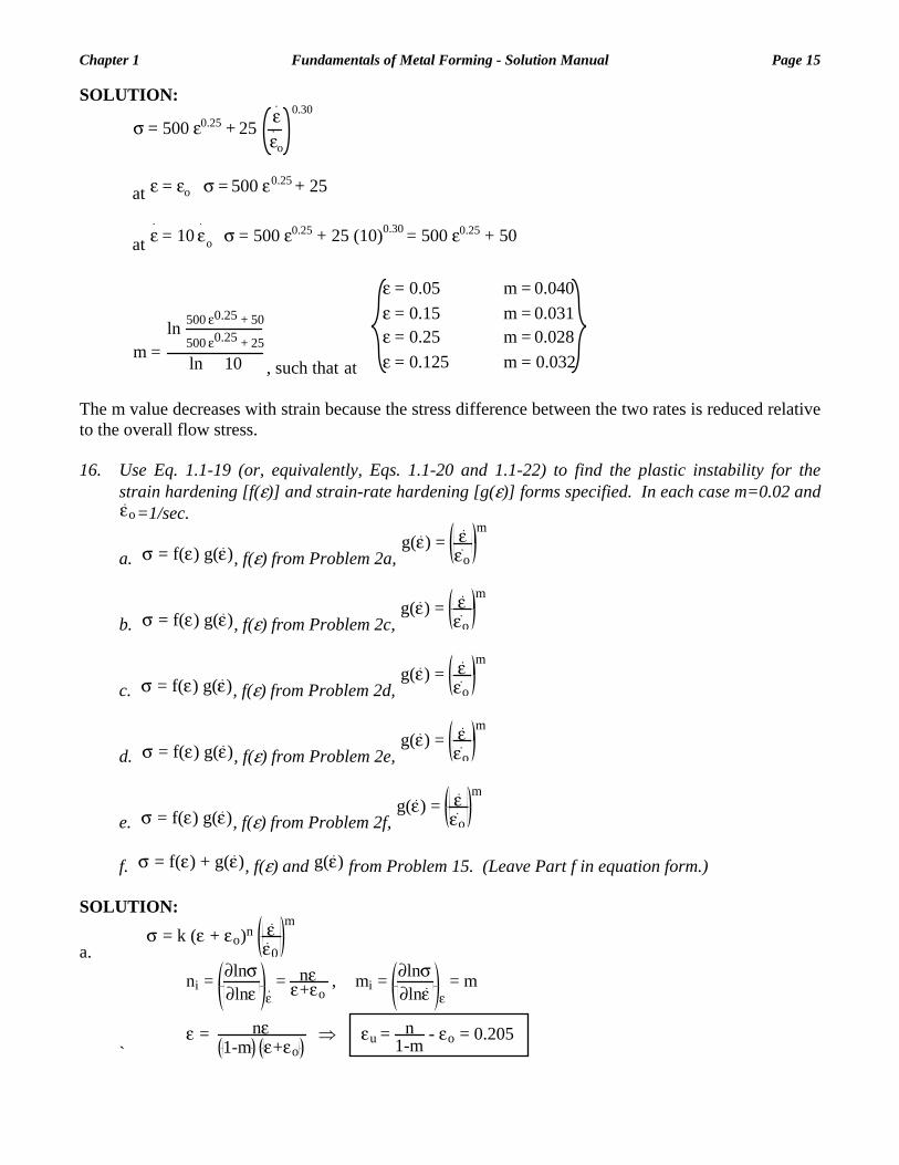
Chapter 1 Fundamentals of Metal Forming - Solution Manual Page 15
SOLUTION:
σ = 500 ε0.25 + 25
εεo
0.30
at
at
ε = εo σ = 500 ε0.25 + 25
ε = 10 εo σ = 500 ε0.25 + 25 (10)0.30 = 500 ε0.25 + 50
m =ln 500 ε0.25 + 50
500 ε0.25 + 25
ln 10 , such that at
ε = 0.05 m = 0.040ε = 0.15 m = 0.031ε = 0.25 m = 0.028ε = 0.125 m = 0.032
The m value decreases with strain because the stress difference between the two rates is reduced relative
6. Use Eq. 1.1-19 (or, equivalently, Eqs. 1.1-20 and 1.1-22) to find the plastic instability for the
to the overall flow stress. 1
strain hardening [f(ε)] and strain-rate hardening [g(ε)] forms specified. In each case m=0.02 and εo=1/sec.
σ = f(ε) g(ε)a. , f(ε) from Problem 2a, g(ε) = ε
εo
m
σ = f(ε) g(ε)b. , f(ε) from Problem 2c, g(ε) = ε
εo
m
σ = f(ε) g(ε)c. , f(ε) from Problem 2d, g(ε) = ε
εo
m
σ = f(ε) g(ε)d. , f(ε) from Problem 2e, g(ε) = ε
εo
m
σ = f(ε) g(ε)e. , f(ε) from Problem 2f, g(ε) = ε
εo
m
f. σ = f(ε) + g(ε), f(ε) and g(ε) from Problem 15. (Leave Part f in equation form.)
OLU ION:
a.
S Tσ = k (ε + εo)n ε
ε0
m
ni = ∂lnσ∂lnε ε
=
n+
εε εo
, mi = ∂lnσ∂lnε ε
= m
`
ε = nε
1-m ε+εo ⇒ εu = n
1-m - εo = 0.205

Page 16 Fundamentals of Metal Forming - Solution Manual Chapter 1
b. σ = σo (1 - Ae
-Bε) εε0
m
ni = ∂lnσ
∂lnε ε = BAε exp(-Bε)
1 - A exp(-Bε) , mi = ∂lnσ
∂lnε ε = m
εu = 1
B ln A (B+1-m)
1-m = 0.300
c. σ = σo ε
ε0
m
ni = ∂lnσ
∂lnε ε = 0 , mi = ∂lnσ
∂lnε ε = m
εu = 0 (Never stable)
d. σ = σo + kε ε
ε0
m
ni = ∂lnσ
∂lnε ε = kε
σo + kε , mi = ∂lnσ
∂lnε ε = m
ε = kε
1-m σo + kε ⇒ εu = 1
1-m - σo
k = 0.306
e. σ = k sin (Bε) ε
ε0
m
ni = ∂lnσ
∂lnε ε = Bε
tan(Bε) , mi = ∂lnσ
∂lnε ε = m
ε = Bε1-m tan(Bε)
⇒ εu = 1B
tan-1 B1-m
= 0.225
f. σ = k εn + B ε
εo
m
ni = ∂lnσ∂lnε ε
= nkεn
kεn + B εεo
m , mi = ∂lnσ∂lnε ε
= Bm ε
εo
m
kεn + B εεo
m
Substitution leads to a transcendental equation:
nεn-1 - εn = B
k (1-m) ε
εo
m ,

Chapter 1 Fundamentals of Metal Forming - Solution Manual Page 17
which may be solved iteratively if so desired. Note that for an additive law such as this one, the plastic instability strain depends on strain rate as well as material constants.

CHAPTER 2 - PROBLEM SOLUTIONS A. PROFICIENCY PROBLEMS 1. Perform the indicated vector operations using the vector components provided:
a ↔ (1, 1, 1) b ↔ (1, 2, 3) c ↔ (-1, 1, -1)a⋅b a×b a⋅(b×c)a⋅c a×c (a×b) ⋅(a×c)b⋅c b×c a⋅(b+c)a+b b×a a⋅b+a⋅ca+c c×a a×(b+c)b+c c×b (a×b)+( a×c)
SOLUTION:
Note: a ⋅ b ↔ ai bi = a1b1 + a2b2 + a3b 3
a × b = εkij ai bj xk = a2b3 – a3b2 x1 + a3b1 – a1b3 x2 + a1b2 – a2b1 x3
a ⋅ b = (1, 1, 1) ⋅ (1, 2, 3) = 1 ⋅ 1 + 1 ⋅ 2 + 1 ⋅ 3 = 6 a ⋅ c = (1, 1, 1) ⋅ (–1, 1, –1) = –1 + 1 – 1 = –1 b ⋅ c = (1, 2, 3) ⋅ (–1, 1, –1) = –1 + 2 – 3 = –2 a + b = (1, 1, 1) + (1, 2, 3) ↔ (2, 3, 4) a + c = (1, 1, 1) + (–1, 1, –1) ↔ (0, 2, 0) b + c = (1, 2, 3) + (–1, 1, –1) ↔ (0, 3, 2)
a × b =x1 x2 x3
1 1 11 2 3
=1 12 3
x1 –1 11 3
x2 +1 11 2
x3 = x1 – 2x2 + x3 ↔ (1, –2, 1)
In a similar way, a × c ↔ (1, –2, 1) b × c ↔ (–2, 0, 2) b × a ↔ (–5, –2, 3) c × a ↔ (2, 0, –2) c × b↔ (5, 2, –3)

Page 2 Fundamentals of Metal Forming - Solution Manual Chapter 2
a ⋅ (b × c) = –4 (a × b)⋅ (a × c) = 0 a ⋅ (b + c) = 5 a ⋅ b + a ⋅ c = 5 a × (b + c) ↔ (–1, –2, 3) (a × b) + (a × c) ↔ (–1, –2, 3)
2. Perform the indicated vector operations.
a. Write the components of the given vectors (a,b,c) n terms of the base vectors x 1
′,x 2′,x 3
′
provided: x1
′ ↔ (0.866, 0.500, 0.000)x2
′ ↔ (-0.500, 0.866, 0.000)x3
′ ↔ (0.000, 0.000, 1.000),
where the components of these base vectors are expressed in the original coordinate system as follows:
a ↔ (1, 1, 1) b ↔ (1, 2, 3) c ↔ ( -1, 1, -1) or
a = x1+x2+x3 b = x1+2x2+3x3 c = -x1+x2-x3 b. Perform the following operations using the components of a, b, c expressed in the new
(primed) basis: a⋅ b a⋅ (b×c) a×(b+c) a×b (a×b)⋅ (a×c) (a×b)+(a×c) a+b
c. Construct the rotation matrix [R] to transform components from the original coordinate
system to the primed coordinate system. Is [R] orthogonal? Find the inverse of [R] in order to transform components expressed in the primed coordinate system back to the original, unprimed coordinate system.
d. Transform the components of the results found in Part b. to the unprimed coordinate system
and compare the results with the equivalent operations carried out in Part a. (using components expressed in the original coordinate system).
SOLUTION: a. x1′ ↔ (0.866, 0.500, 0.000) x1′ = 0.866 x1 + 0.5 x2
x2′ ↔ (–0.500, 0.866, 0.000) x2
′ = – 0.5 x1 + 0.866 x2 x3
′ ↔ (0.000, 0.000, 1.000) x3' = x3
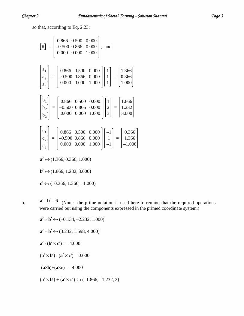
Chapter 2 Fundamentals of Metal Forming - Solution Manual Page 3
so that, according to Eq. 2.23:
R =0.866 0.500 0.000–0.500 0.866 0.0000.000 0.000 1.000
, and
a1′
a2′
a3′
=0.866 0.500 0.000–0.500 0.866 0.0000.000 0.000 1.000
111
=1.3660.3661.000
b1′
b2′
b3′
=0.866 0.500 0.000–0.500 0.866 0.0000.000 0.000 1.000
123
=1.8661.2323.000
c1′
c2′
c3′
=0.866 0.500 0.000–0.500 0.866 0.0000.000 0.000 1.000
–11–1
=0.3661.366–1.000
a′ ↔ (1.366, 0.366, 1.000) b′ ↔ (1.866, 1.232, 3.000) c′ ↔ (–0.366, 1.366, –1.000)
b. (Note: the prime notation is used here to remind that the required operations
were carried out using the components expressed in the primed coordinate system.) a′ ⋅ b′ = 6
a′ × b′ ↔ (–0.134, –2.232, 1.000) a′ + b′ ↔ (3.232, 1.598, 4.000) a′ ⋅ (b′ × c′) = –4.000 (a′ × b′) ⋅ (a′ × c′) = 0.000 (a×b)+(a×c) = –4.000 (a′ × b′) + (a′ × c′) ↔ (–1.866, –1.232, 3)

Page 4 Fundamentals of Metal Forming - Solution Manual Chapter 2
c.
R =
0.866 0.500 0.000–0.500 0.866 0.0000.000 0.000 1.000
, x′ = R x
R RT =
0.866 0.500 0.000–0.500 0.866 0.0000.000 0.000 1.000
0.866 –0.500 0.0000.500 0.866 0.0000.000 0.000 1.000
=1.00 0.00 0.000.00 1.00 0.000.00 0.00 1.00
= I
Orthogonal
R –1 =
signedcofactormatrix
–1
A=
0.866 –0.500 0.0000.500 0.866 0.0000.000 0.000 1.000
= R T
d. a ′ = R a , or
R –1 a ′ = a (i) a ⋅ b = 6 ; does not change since it is scalar.
(ii)
a × b =
0.866 –0.500 0.0000.500 0.866 0.0000.000 0.000 1.000
–0.134–2.2321.000
=1–21
↔ (1, –2, 1) (same result)
(iii)
a + b =
0.866 –0.500 0.0000.500 0.866 0.0000.000 0.000 1.000
3.2321.5984.000
=234
↔ (2, 3, 4) (same result)
(iv) a ⋅ (b × c) = a ⋅ (b × c) = –4 (v) a ⋅ (b × c) = a ⋅ (b × c) = 0 (vi) (a × b) ⋅ (a × c) = (a × b) ⋅ (a × c) ↔ (–1, –2, 3) (vii) a × (b + c) = a × (b + c) ↔ (–1, –2, 3) (viii) (a × b) + (a × c) = (a × b) + (a × c) ↔ (–1, –2, 3) Should have the same results for every case.
3. Find the rotation matrices for the following operations:
a. Rotation of axes (i.e. component transformation) 45 about ° x3 in a right-handed sense (counter-clockwise when looking anti-parallel along x3).
b. Rotation of a physical vector 45 about ° x3 in a right-handed sense (i.e. the vector moves

Chapter 2 Fundamentals of Metal Forming - Solution Manual Page 5
counter-clockwise when looking anti-parallel along x3). c. Rotation of axes (i.e. component transformation) 30 about ° x2 in a right-handed sense (i.e.
counter-clockwise when viewed anti-parallel to x2). d. Rotation of a physical vector 30 about ° x2 in a right-handed sense (i.e. the vector moves
counter-clockwise when looking anti-parallel along x2).
SOLUTION: a.
R =
cos 45° cos 45° cos 90°
cos 135° cos 45° cos 90°
cos 90° cos 90° cos 0°
=
22
22 0
–22
22
0
0 0 1
b.
R =
22 –
22 0
–2
22
20
0 0 1 c.
R =
32 0 –
12
0 1 0
12
0 32
d.
R =
32 0 –
12
0 1 0
– 12
0 32
4. Perform the matrix manipulations shown. a. Find the determinants and inverses of the following matrices:
A =
1 2 34 5 67 8 9
B =7 8 91 2 34 5 6
C =1 1 1-1 2 33 1 -1
b. Multiply A A -1, B B -1, and C C -1 to verify that the inverse has been correctly
obtained. SOLUTION:
a.
A =
1 2 34 5 67 8 9
B =7 8 91 2 34 5 6
C =1 1 1–1 2 33 1 –1
A = 1 (5 ⋅ 9 – 6 ⋅ 8) – 4 (2 ⋅ 9 – 3 ⋅ 8) + 7 (2 ⋅ 6 – 3 ⋅ 5) = 0

Page 6 Fundamentals of Metal Forming - Solution Manual Chapter 2
A –1 =
signed wfactormatrix
T
A, since A = 0, A –1 cannot be obtained
B = A = 0, B –1 → does not exist
C = 1 (–2 –3) – 1 (1 – 9) + 1 (–1 – 6) = –4,
C –1 =1.25 –0.5 –0.25–2 1 1
1.75 –0.5 –0.75
b. A A –1 , B B –1 ; not applicable.
C C –1 =1 1 1
–1 2 33 1 –1
1.25 –0.5 –0.25–2 1 1
1.75 –0.5 –0.75=
1 0 00 1 00 0 1
Yes, inverse has been correctly obtained. ∴
5. The following sets of basis vectors are presented in a standard Cartesian coordinate system
(x1, x2, x3).
Set (1)
x1(1)
↔ 0.707, 0.707, 0.000
x2(1)
↔ -0.500, 0.500, 0.707
x3(1)
↔ 0.500, -0.500, 0.707
Set (2)
x1(2)
↔ 0.750, 0.433, 0.500
x2(2)
↔ -0.500, 0.866, 0.000
x3(2)
↔ -0.433, -0.250, 0.866
Set (3)
x1(3)
↔ 0.866, 0.500, 0.354
x2(3)
↔ 0.500, 0.866, 0.354
x3(3)
↔ 0.000, 0.000, 0.866
a. Using vector operations, determine which of the basis sets are orthogonal. b. Determine the transformation matrices to transform components presented in the original
coordinate system (x1, x2, x3) to those in each of the other basis systems.

Chapter 2 Fundamentals of Metal Forming - Solution Manual Page 7
c. Which of the transformation matrices in Part b. are orthogonal? Does this agree with Part a?
d. Find the transformation matrix to transform components provided in coordinate system (1)
to components expressed in coordinate system (2). Is the transformation matrix orthogonal?
SOLUTION: a. To be orthogonal, the inner product of two vectors should be zero.
Set (1) x1
(1)⋅ x2
(1)= (0.707, 0.707, 0.000) ⋅ (-0.5, 0.5, 0.707) = 0.0
x3(1)
⋅ x2(1)
= (0.500, -0.500, 0.707) ⋅ (-0.500, 0.500, 0.707) = 0.0
x1(1)
⋅ x3(1)
= (0.707, 0.707, 0.000) ⋅ (0.500, -0.500, 0.707) = 0.0
∴ orthogonal
Set (2) x1(2)
⋅ x2(2)
= x2(2)
⋅ x3(2)
= x1(2)
⋅ x3(2)
= 0.0 ∴ orthogonal
Set (3) x2(3)
⋅ x3(3)
= 0.991
x1(3)
⋅ x2(3)
= 0.307
x1(3)
⋅ x3(3)
= 0.307 ∴ not orthogonal
b. x1 ↔ (1, 0, 0) , x2 ↔ (0, 1, 0) , x3 ↔ (0, 0, 1)
Set(1)
x1
(1)↔ (0.707, 0.707, 0.0) = 0.707 (1, 0, 0) + 0.707 (0, 1, 0) + 0.0 (0, 0, 1)
x2(1)
↔ (-0.5, 0.5, 0.707) = -0.5 (1, 0, 0) + 0.5 (0, 1, 0) + 0.707 (0, 0, 1)
x3(1)
↔ (0.5, -0.5, 0.707) = 0.5 (1, 0, 0) + -0.5 (0, 1, 0) + 0.707 (0, 0, 1)
In a similar way as shown in Exercise 2.5, we obtain
Set (1)
R(1) =
0.707 0.707 0.000–0.500 0.500 0.7070.500 –0.500 0.707
Set (2)
R(2) =
0.750 0.433 0.500–0.500 0.866 0.000–0.433 –0.250 0.866
Set (3)
R(3) =
0.866 0.500 0.3540.500 0.866 0.3540.000 0.000 0.866
Page 8 Fundamentals of Metal Forming - Solution Manual Chapter 2
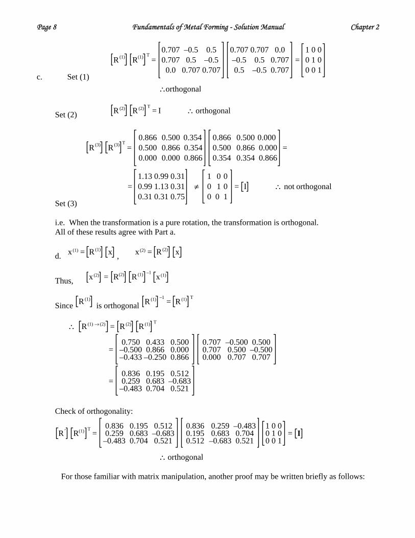
c. Set (1)
R(1) R(1) T=
0.707 –0.5 0.50.707 0.5 –0.5
0.0 0.707 0.707
0.707 0.707 0.0–0.5 0.5 0.7070.5 –0.5 0.707
=1 0 00 1 00 0 1
∴orthogonal
Set (2) R(2) R(2) T
= I ∴ orthogonal
Set (3)
R(3) R(3) T=
0.866 0.500 0.3540.500 0.866 0.3540.000 0.000 0.866
0.866 0.500 0.0000.500 0.866 0.0000.354 0.354 0.866
=
=1.13 0.99 0.310.99 1.13 0.310.31 0.31 0.75
≠1 0 00 1 00 0 1
= I ∴ not orthogonal
i.e. When the transformation is a pure rotation, the transformation is orthogonal. All of these results agree with Part a.
d. x(1) = R(1) x ,
x(2) = R(2) x
Thus, x (2) = R(2) R(1) –1
x(1)
Since R(1)
is orthogonal R(1) –1
= R(1) T
∴ R(1) → (2) = R(2) R(1) T
=
0.750 0.433 0.500–0.500 0.866 0.000–0.433 –0.250 0.866
0.707 –0.500 0.5000.707 0.500 –0.5000.000 0.707 0.707
=
0.836 0.195 0.5120.259 0.683 –0.683–0.483 0.704 0.521
Check of orthogonality:
R ′ R(1) T
=0.836 0.195 0.5120.259 0.683 –0.683
–0.483 0.704 0.521
0.836 0.259 –0.4830.195 0.683 0.7040.512 –0.683 0.521
1 0 00 1 00 0 1
= I
∴ orthogonal For those familiar with matrix manipulation, another proof may be written briefly as follows:
Chapter 2 Fundamentals of Metal Forming - Solution Manual Page 9
R(1) R(1) T= R(2) R(1) T
R(2) R(1)T
= R(2) R(1) TR(1) R(2) T
= R(2) R(2) T= I
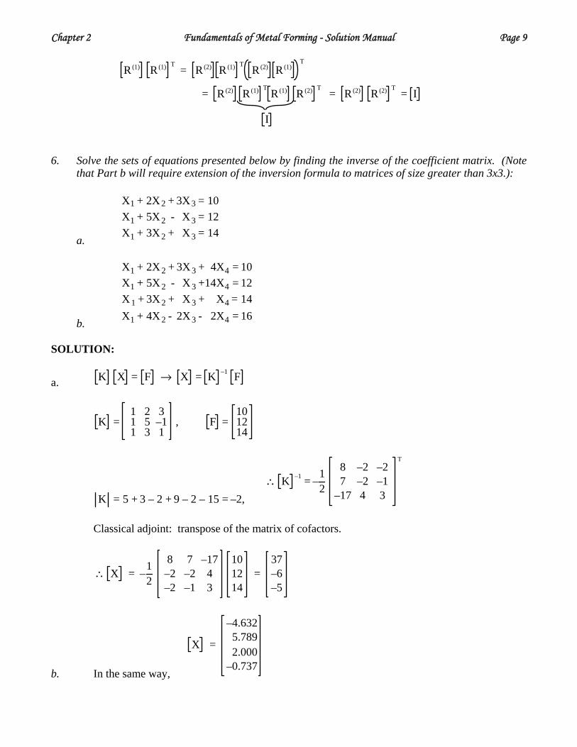
I 6. Solve the sets of equations presented below by finding the inverse of the coefficient matrix. (Note
that Part b will require extension of the inversion formula to matrices of size greater than 3x3.):
a.
X1 + 2X2 + 3X3 = 10X1 + 5X2 - X3 = 12X1 + 3X2 + X3 = 14
b.
X1 + 2X 2 + 3X3 + 4X4 = 10X1 + 5X 2 - X3 +14X4 = 12X1 + 3X2 + X3 + X4 = 14X1 + 4X 2 - 2X3 - 2X4 = 16
SOLUTION:
a. K X = F → X = K –1 F
K =
1 2 31 5 –11 3 1
, F =101214
K = 5 + 3 – 2 + 9 – 2 – 15 = –2,
∴ K –1 = –12
8 –2 –27 –2 –1
–17 4 3
T
Classical adjoint: transpose of the matrix of cofactors.
∴ X = –12
8 7 –17–2 –2 4–2 –1 3
101214
=37–6–5
b. In the same way,
X =
–4.6325.7892.000
–0.737

Page 10 Fundamentals of Metal Forming - Solution Manual Chapter 2 7. Perform the following operations related to eigenvector - eigenvalue problems.
a. Find the eigenvalues and the associated eigenvectors for the following matrices:
1 23 1
1 2 32 4 53 5 6
1 -1 2-1 2 -32 -3 3
b. Find the transformation matrices which change components expressed in the original
coordinate system to ones expressed using the eigenvectors as base vectors. Choose the direction associated with the maximum eigenvalue to be the new x1' ,the second one x2' , and the third one x3' .
c. Treating the columns of the matrices in part a. as vectors, find the equivalent components
expressed in the eigenvector bases from Part b.. [i.e. use the transformation matrices found in Part c. to find the new components of the tensors in Part a., expressed in the principal coordinate system.]
SOLUTION:
a. A – λI = 0 ,
1–λ 23 1–λ
= 1–λ 2 – 6 = 1–2λ + λ2 – 6 = λ2–2λ – 5 = 0
Eigenvalues: λ1 = 1 + 6 , λ2 = 1 – 6 ; Eigenvectors: p(1) , p(2)
(i) For λ = 1 + 6 = 3.449 ,
p(1) ↔
x1(1)
x2(1)
A – λ 1 I p(1) =
– 6 23 – 6
x1(1)
x2(1) =
00
Let x1(1) = 1, then – 6 + 2x2
(1) = 0
∴ x2
(1) =6
2
Normalizing these
p(1) ↔ 1
52
1, 62 = (0.632, 0.775)
(ii) For λ = 1 – 6 = –1.449
6 23 6
x1(2)
x2(2) =
00
,
and if x1
(2) = 1, then x2(2) = – 6
2 Normalizing, we get p(2) ↔ (0.632, – 0.775)

Chapter 2 Fundamentals of Metal Forming - Solution Manual Page 11
Check of orthogonality: (Not orthogonal because the
original p(1) ⋅ p(2) = – 0.20 ≠ 0
matrix is not symmetric.) Using the same procedure,
(ii) For
1 2 32 4 53 5 6 ,
λ1 = 11.345, p1 ↔ (0.328, 0.591, 0.737)λ2 = –0.516, p2 ↔ (0.737, 0.328, –0.591)λ3 = 0.171, p3 ↔ (–0.591, 0.737, –0.328)
(iii)
1 –1 2–1 2 –32 –3 3 ,
λ1 = 6.419, p1 ↔ (0.374, –0.577, 0.725)λ2 = –0.387, p2 ↔ (0.816, 0.577, 0.038)λ3 = 0.806, p3 ↔ (–0.441, 0.577, 0.687)
b.
T (1) = 0.632 0.775
0.632 – 0.775
T (2) =
0.328 0.591 0.737–0.591 0.737 –0.3280.737 0.328 –0.591
T (3) =
0.374 –0.577 0.7250.816 0.577 0.038–0.041 0.577 0.687
c. Suppose x, y, z are orthogonal eigenvectors of A where eigenvalues are respectively, let
λ1, λ2, and λ3,
L =
x1 y1 z1x2 y2 z2x3 y3 z3 , where
x ↔
x1x2x3
y ↔y1y2y3
z ↔z1z2z3
Then from 2.35a,
A x = λ1 xA y = λ2 yA z = λ3 z
→ A L = D L ∴ D = L T A L
Here L = T T, and D = T A T T
We will obtain [D]; the diagonal matrix whose diagonal components are eigenvalues. For example,

Page 12 Fundamentals of Metal Forming - Solution Manual Chapter 2
D =0.328 0.591 0.7370.737 0.328 –0.591–0.591 0.737 –0.328
1 2 32 4 53 5 6
0.328 0.737 –0.5910.591 0.328 0.7370.737 –0.591 –0.328
=11.345 0 0
0 –0.516 00 0 0.171
8. Find the new components of the tensors provided below if the coordinate system change
corresponds to a rotation of 30 about ° x3:
R =0.866 0.500 0.000
-0.500 0.866 0.0000.000 0.000 1.000
T1 ↔ 1 2 32 4 53 5 6
= T1 , T2 ↔ 1 2 34 5 67 8 9
= T2
SOLUTION:
T ′ = R T R T , T1′ = R T1 R T , T2
′ = R T R2T
T1′ =
0.866 0.500 0.000–0.500 0.866 0.0000.000 0.000 1.000
1 2 32 4 53 5 6
0.866 –0.500 0.0000.500 0.866 0.0000.000 0.000 1.000
=3.482 2.299 5.0982.299 1.518 2.8305.098 2.830 6.000
T2
′ = R T2 R T =4.598 2.232 5.5984.232 1.402 3.69610.062 3.428 9.000
9. In calculating contact conditions at an interface, it is often necessary to find the unit vector which
represents the projection of a given vector (usually the displacement of a material point) onto a plane tangent to the interface. If the normal to the tangent plane is denoted n and the arbitrary vector is a, find t, the unit tangent vector corresponding to the material displacement. [Express the result in terms of a, n̂ , and simple vector operations.]
SOLUTION:
One possibility is based on the use of vector addition and the dot product:
t =
a – a ⋅ n na – a ⋅ n n
(since t is a unit vector)
Alternatively, one may use the cross product to accomplish the same thing by first defining a
unit vector q , which is orthogonal to n , a , and t :
q = a × n
a × n ,
t = n × q =
n × a × n
a × n B. DEPTH PROBLEMS

Chapter 2 Fundamentals of Metal Forming - Solution Manual Page 13 10. Perform the following operations related to component transformations.
a. Find the transformation for components from basis set (2) to basis set (3), in Problem 5, above.
b. Find the inverse transformation, that is, one that expresses components in basis set (2) if
they are given in basis set (3). c. Using the approach shown in Exercise 2.5, verify that transformation matrices found in
Parts a. and b. do, indeed, perform the indicated transformations. d. Show the matrix form of the tensor transformation for components given in basis set (2) to
those in basis set (3).
SOLUTION:
a. xi
(2) → xi(3)
x(2) = R(2) x ,
x = R(2) Tx2
x(3) = R(3) x ,
x3 = R(3) R(2) Tx(2)
∴ R(2)→(3) = R(3) R(2) T =
0.866 0.500 0.3540.500 0.866 0.3540.000 0.000 0.866
0.750 – 0.500 – 0.4330.433 0.866 – 0.2500.500 0.000 0.866
=1.043 0.000 – 0.1930.927 0.500 – 0.1260.433 0.000 0.750
Since the inverse of R(3)
is not used in this transformation, its non-orthogonality is not an issue. However, in part b this requires inverting (rather than transposing) a matrix.
b. Recall from Part a: R(2)→(3) = R(3) R(2) T
R(2)→(3) –1
= R(3) R(2) T –1
= R(2) R(3) – 1=
0.866 0.000 0.223– 1.732 2.000 – 0.110– 0.500 0.000 1.204
Where we have used the relationships: R(2) – 1
= R(2) Tand A B
– 1= B – 1 A – 1
c. Let's verify the transformations by considering three vectors, namely those of the original basis set x i
(o)(let's label them x , y, x here to simplify the notation). We form the matrix
A (corresponding to the tensor A composed of the three vectors) in the usual way, by putting the components of each basis vector into a column. Since we are considering the
components of the basis set in the basis set, A is the identity matrix:

Page 14 Fundamentals of Metal Forming - Solution Manual Chapter 2
A ↔ A(o) =x1
(o) y1(o) z1
(o)
x2(o) y2
(o) z2(o)
x3(o) y3
(o) z3(o)
=1 0 00 1 00 0 1
= I
We then find the coordinates of these three vectors expressed in the x (2) and x (3)
basis sets:
A ↔ A(2) = R(2) I =
0.750 0.433 0.500–0.500 0.866 0.000–0.433 –0.250 0.866
(in basis set 2)
A ↔ A(3) = R(3) I =
0.866 0.500 0.3540.500 0.866 0.3540.000 0.000 0.866
(in basis set 3)
Now, our transformation matrix R(2)→(3)
must transform the components of any vector expressed in x i
(2) to components expressed in x i
(3):
A (3) = R(2)→(3) A (2) =
1.043 0.000 – 0.1930.927 0.500 – 0.1260.433 0.000 0.750
0.750 0.433 0.500–0.500 0.866 0.000–0.433 –0.250 0.866
=0.866 0.500 0.3540.500 0.866 0.3540.000 0.000 0.866
= A(3)
Comparison of A(3)
obtained here with A(3)
above shows that the transformation matrix R(2)→(3)
performs its intended function. R(3)→(2)
, the inverse of R(2)→(3)
may be verified in the same manner.
d. Shown in a. 11. Find the rotation matrix for the double rotation of coordinate axes: rotate 90 about ° x1, and then
about 90° x3. SOLUTION:
R1 =
1 0 00 0 10 –1 0
R2 =
0 1 0–1 0 00 0 1
Chapter 2 Fundamentals of Metal Forming - Solution Manual Page 15
R = R2 R1 =0 1 0–1 0 00 0 1
1 0 00 0 10 –1 0
0 0 1–1 0 00 –1 0
R 1–2 =
0 0 1–1 0 00 –1 0
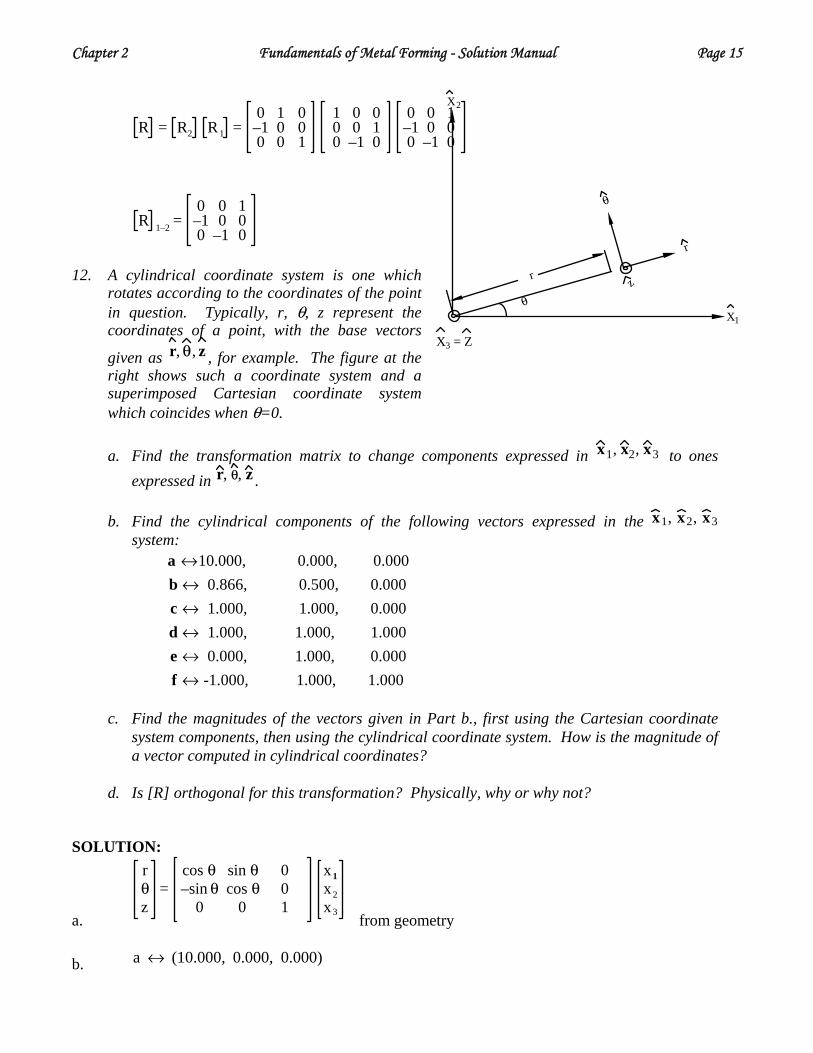
12. A cylindrical coordinate system is one which
rotates according to the coordinates of the point in question. Typically, r, θ, z represent the coordinates of a point, with the base vectors
given as r, θ, z , for example. The figure at the right shows such a coordinate system and a superimposed Cartesian coordinate system which coincides when θ=0.
X1
θ
r
zr
θ
X3 = Z
X2
a. Find the transformation matrix to change components expressed in x1, x2, x3 to ones
expressed in r, θ, z . b. Find the cylindrical components of the following vectors expressed in the x1, x2, x3
system:
a ↔10.000, 0.000, 0.000b ↔ 0.866, 0.500, 0.000c ↔ 1.000, 1.000, 0.000d ↔ 1.000, 1.000, 1.000e ↔ 0.000, 1.000, 0.000f ↔ -1.000, 1.000, 1.000
c. Find the magnitudes of the vectors given in Part b., first using the Cartesian coordinate
system components, then using the cylindrical coordinate system. How is the magnitude of a vector computed in cylindrical coordinates?
d. Is [R] orthogonal for this transformation? Physically, why or why not?
SOLUTION:
a.
rθz
=cos θ sin θ 0–sin θ cos θ 0
0 0 1
x 1x2x3
from geometry
b. a ↔ (10.000, 0.000, 0.000)

Page 16 Fundamentals of Metal Forming - Solution Manual Chapter 2
a = R x
a1
a2
a3
=cos θ sin θ 0–sin θ cos θ 0
0 0 1
1000
=10 cos θ–10 sin θ
0 In a similar way,
b =0.866 cos θ + 0.5 sin θ–0.866 sin θ + 0.5 cos θ
0
c =cos θ + sin θ
–sin θ + cos θ0
d =cos θ + sin θ–sin θ + cos θ
1
e =
sin θcos θ
0
f =–cos θ + sin θsin θ + cos θ
1
c. Cartesian Coordinate Cylindrical Coordinate
a = 102 + 02 + 02 = 10 a = 102 cos2θ + 102 sin2θ = 10
Likewise, should have the same results.
d.
R R T =cos θ sin θ 0–sin θ cos θ 0
0 0 1
cos θ –sin θ 0sin θ cos θ 0
0 0 1= I
The basis sets of each system are mutually orthogonal.
13. Perform the indicated operations related to equation solving.
a. Solve the equations given in Problem 6 by using Gaussian reduction instead of by finding the inverse. Which to you prefer for large matrices?
b. Given the solutions obtained in Part a., find the inverse of the coefficient matrix. c. For larger sets of equations, why is it easier to solve by a reduction method?
SOLUTION:
a.
1 2 31 5 –11 3 1
101214
→1 2 30 3 –40 1 –2
1024
→1 2 30 3 –4
0 –23
102103
∴
x3 = –5x2 = –6x1 = 37
Similarly, we should get the same results for the second set. The Gassian reduction method

Chapter 2 Fundamentals of Metal Forming - Solution Manual Page 17
is much simpler for large matrices because it operates row-by-row and it is not necessary to keep track of complex expressions.
b. Solutions given in Problem 6.
c. For large sets of equations, it is much more complicated to compute the inverse of a matrix,
whereas the reduction method does not involve inverse computation. Less computation is required in a reduction method.

CHAPTER 3 - PROBLEM SOLUTIONS A. PROFICIENCY PROBLEMS 1. Calculate the 3-D stress tensor components for the rectangular material shown in the figure, first
in the coordinate system x1, x2, and x3 and then in the coordinate system x1', x2', x 3' .
X3
200 N
X1
X2
X1'X2'
X3'1 mm
1 mm
The angle between x1′and x1 is 30o, and the x3
′and x3 axes are parallel.
SOLUTION: Before doing the problem formally using the known tensor transformations, let's approach it from a physical and geometrical standpoint. Because of the equilibrium, we know that the force transmitted throught the cross-sectional area (1mm2) normal to x1 is 200N, and the stress vector
operating on that same plane is S1 ↔ (200, 0, 0) N
mm2 . The other two planes, normal to x2 and x3, contain the force vector and thus have no associated stress vectors:
.
S 2 ↔ (0, 0, 0)S 3 ↔ (0, 0, 0)
Therefore, the stress tensor in the x i coordinate system may be written:
σ ↔
200 0 00 0 00 0 0
.
The situation in the x i
′ coordinate system may be approached similarly by first considering the
plane normal to x1′ which passes through the rod. The entire 200N of force must be transmitted
through this area, which is now larger because of the incline:
A 1
′ = 1mm 2
cos 30° = 1.155mm2
The corresponding stress vector thus has a magnitude of
S 1
′ = 200 N1mm2 cos 30° = 200 N
1.155 mm 2 = 173.2 N/mm2,
To find the components of this vector along the x1' and x2' vectors, we simply resolve this value:
S1′ ↔ (173.2 cos 30, 173.2 sin 30, 0) = (150, 86.6, 0) N
mm2 To find the stress vector operating on the plane normal to x2
′, we follow the same procedure:
A 2
′ = 1mm2
sin 30° = 2 mm2,, so
S 2′ = 100 N/mm2,

Page 2 Fundamentals of Metal Forming - Solution Manual Chapter 3
and the associated stress vector components are S2
′ ↔ (100 cos 30, 100 sin 30, 0) = (86.6 N/mm2, 50 N/mm 2, 0) And the entire stress tensor in x1' is
S 1'′ S 2'
′ S 3'′
σ =150 86.6 086.6 50 0
0 0 0
It is much easier and less error-prone to use the known tensor transformation properties to solve the problem, as follows: Let σ be the stress tensor in the material and t the stress vector, then we have in general:
σ ⋅ n = t = F
a .
For n = x 1 , we get:
t1 = σ ⋅ x 1 = F
a , so that t1 =200 0 00 0 00 0 0
MPa
Similarly, t2 = σ ⋅ x 2 , t3 = σ ⋅ x 3 , and we can conclude that the stress tensor is
σ =200 0 00 0 00 0 0
MPa
In order to transform these components to those corresponding to the x1′
coordinate system, we first find the rotation matrix:
x ′ = R x ⇒
x1′
x2′
x3′
=
32
–12 0
12
32 0
0 0 1
x1
x2
x3
and then apply the transformation rule for a second-ranked tensor:
σ′ = R σ R T ⇒
32
–12 0
12
32 0
0 0 1
200 0 0
0 0 0
0 0 0
32
12 0
–12
32 0
0 0 1

Chapter 3 Fundamentals of Metal Forming - Solution Manual Page 3
=
100 3 0 0
100 0 0
0 0 0
32
12 0
–12
32 0
0 0 1
=
150 50 3 0
50 3 50 0
0 0 0
=
150 86.6 0
86.6 50 0
0 0 0
MPa
2. Given the stress tensor which appears below, find the stress vector acting on planes normal to the
unit vectors n, m , and p , also given.
σ ↔ 1 2 32 2 43 4 3
n ↔ 13 (1,1,1)
m ↔ 16 (1,2,1)
p ↔ 12 (1,1,0)
SOLUTION:
t = σ n
t n =
1 2 3
2 2 4
3 4 3
13
13
13
=
63
83
103
=
3.464
4.619
5.774
t m =
1 2 3
2 2 4
3 4 3
16
26
16
=
86
106
156
=
3.266
4.082
5.715
t p =
1 2 3
2 2 4
3 4 3
1212
0
=
32
42
72
=
2.121
2.828
4.950
3. Find the principal stresses, the principal directions, and the rotation matrix for transforming
coordinates to the principal coordinate system ( x1′ corresponds to σmax,
x3′ corresponds to σmin)
for the stress tensors given.
a.3 -1 0
- 1 3 00 0 1
, b.3 0 00 3 - 10 - 1 1
, c.10 -5 5- 5 0 55 5 10
Note: No numerical procedure is required to find the roots of the cubic equations.
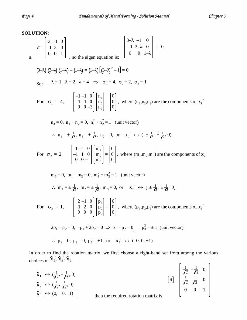
Page 4 Fundamentals of Metal Forming - Solution Manual Chapter 3 SOLUTION:
a.
σ =
3 –1 0–1 3 00 0 1
, so the eigen equation is:
3–λ –1 0–1 3–λ 00 0 1–λ
= 0
3–λ 3–λ 1–λ – 1–λ = 1–λ 3–λ 2 – 1 = 0 So: λ = 1, λ = 2, λ = 4 ⇒ σ 1 = 4, σ2 = 2, σ3 = 1
For σ1 = 4,
–1 –1 0–1 –1 00 0 –3
n1n2n3
=000
, where (n1,n2,n3) are the components of x1′
n3 = 0, n1 + n2 = 0, n12 + n2
2 = 1 (unit vector)
∴ n1 = ± 1
2 , n2 = + 12 , n3 = 0, or x1
′ ↔ ( ± 12
, + 12
, 0)
For σ 2 = 2
1 –1 0–1 1 00 0 –1
m1m2m3
=000
, where (m1,m2,m3) are the components of x2′
m3 = 0, m1 – m2 = 0, m12 + m2
2 = 1 (unit vector)
∴ m1 = ± 1
2 , m2 = ± 12 , m 3 = 0, or x2
′ ↔ ( ± 12
, ± 12
, 0)
For σ3 = 1,
2 –1 0–1 2 00 0 0
p1p2p3
=000
, where (p1,p2,p3) are the components of x3′
, 2p1 – p2 = 0, –p1 + 2p2 = 0 ⇒ p1 = p2 = 0 p32 = ± 1 (unit vector)
∴ p1 = 0, p2 = 0, p3 = ±1, or x3
′ ↔ ( 0, 0, ±1) In order to find the rotation matrix, we first choose a right-hand set from among the various choices of x1
′, x2′, x3
′
x1′ ↔ ( 1
2, – 1
2, 0)
x2′ ↔ ( 1
2,
12
, 0)
x3′ ↔ (0, 0, 1) , then the required rotation matrix is
R =
12
– 12
012
12
0
0 0 1

Chapter 3 Fundamentals of Metal Forming - Solution Manual Page 5
b.
σ =3 0 00 3 –10 –1 1
, so the eigen equation is3–λ 0 0
0 3–λ –10 –1 1–λ
= 0
3 – λ 3 – λ 1 – λ – 1 = 0
So, λ1 = 3, λ2,3 = 4 ± 8
2 = 3.41, 0.59 ⇒ σ 1 = 3.414, σ 2 = 3.000, σ 3 = 0.586
For σ1 = 3.41,
–0.41 0 00 –0.41 –10 –1 –2.41
n1n2n3
=000
, where (n1,n2,n3) are the components of x1′
n1 = 0, –0.41 n2 – n3 = 0, n1
2 + n22 + n3
2 = 1 ∴ x1
′ ↔ (0, ±0.92, +−0.38)
For σ2 = 3,
0 0 00 0 –10 –1 –2
m1m2m3
=000
, where (m1,m2,m3) are the components of x2′
m3 = 0, m2 = 0, m1 = ±1
∴ x2
′ ↔ (±1, 0, 0)
For σ3 = 0.586,2.414 0 0
0 2.414 –10 –1 0.414
p1
p2
p3
=000
, where (p1,p2,p3) are the components of x 3′
p1 = 0, 2.414 p2 – p3 = 0, p1
2 + p22 + p3
2 = 1
∴ x3
′ ↔ (0, ±0.38, ±0.92) In order for find the rotation matrix we first choose a right-handed set of eigenvectors:
x1′ ↔ (0, 0.92, –0.38)
x2′ ↔ (1, 0, 0)
x3′ ↔ (0, –0.38, –0.92) then the rotation matrix is
R =0 0.92 –0.381 0 00 –0.38 –0.92
c.
σ =
10 –5 5–5 0 55 5 10
⇒ σ1 = 15, σ2 = 10, σ3 = –5

Page 6 Fundamentals of Metal Forming - Solution Manual Chapter 3
x1′ ↔ 0.707, 0, 0.707 , for σ1 = 15
x2′ ↔ 0.577, –0.577, –0.577 , for σ 2 = 10
x3′ ↔ 0.408, 0.816, –.408 , for σ3 = –5
R =.707 0 .707.577 –.577 –.577.408 .816 –.408
Check:
R σ R T =σ1 0 00 σ2 00 0 σ3
R σ =10.6 0 10.65.77 –5.77 –5.77
–2.04 –4.08 2.04
R σ R T =
15 0 00 10 00 0 –5
4. Find the invariants for the stress tensors shown below:
a.1.44 0.22 -0.760.22 2.25 -0.38
-0.76 -0.38 2.31, b.
1.75 0.35 -0.750.35 2.50 -0.35
-0.75 -0.35 1.75, c.
1.94 0.38 -0.540.38 2.75 – 0.22-0.54 -0.22 1.31
SOLUTION:
a.
σ =1.44 0.22 –0.760.22 2.25 –0.38
–0.76 –0.38 2.31
J1 = σ11 + σ22 + σ33 = 1.44 + 2.25 + 2.31 = 6
J 2 = – σ11 σ22 + σ22 σ33 + σ33 σ11 + σ232 + σ31
2 + σ122
= – 1.44 2.25 + 2.25 2.31 + 2.31 1.44 + –0.38 2 + –0.76 2 + 0.22 2 = –11
J3 =1.44 0.22 –0.760.22 2.25 –0.38
–0.76 –0.38 2.31= 6
b.
σ =1.75 0.35 –0.750.35 2.50 –0.35
–0.75 –0.35 1.75
J 1 = 6J 2 = –11J 3 = 6
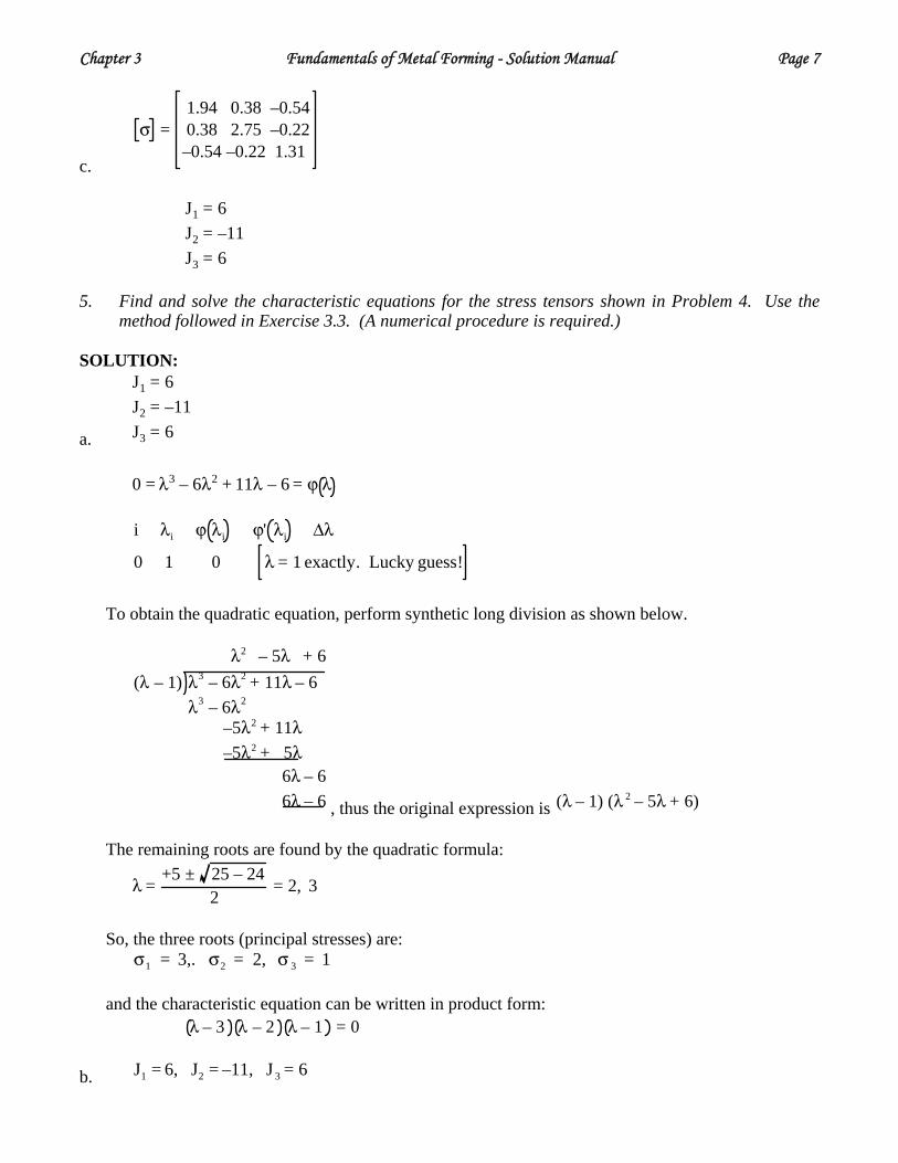
Chapter 3 Fundamentals of Metal Forming - Solution Manual Page 7
c.
σ =1.94 0.38 –0.540.38 2.75 –0.22
–0.54 –0.22 1.31
J1 = 6J2 = –11J3 = 6
5. Find and solve the characteristic equations for the stress tensors shown in Problem 4. Use the
method followed in Exercise 3.3. (A numerical procedure is required.) SOLUTION:
a.
J1 = 6J2 = –11J3 = 6
0 = λ3 – 6λ2 + 11λ – 6 = ϕ λ
i λi ϕ λi ϕ' λi Δλ
0 1 0 λ = 1 exactly. Lucky guess!
To obtain the quadratic equation, perform synthetic long division as shown below.
λ3 – 6λ2 + 11λ – 6(λ – 1)
λ2 – 5λ + 6
λ3 – 6λ2
–5λ2 + 11λ–5λ2 + 5λ
6λ – 66λ – 6 , thus the original expression is (λ – 1) (λ 2 – 5λ + 6)
The remaining roots are found by the quadratic formula:
λ =
+5 ± 25 – 242
= 2, 3
So, the three roots (principal stresses) are: σ1 = 3,. σ2 = 2, σ 3 = 1 and the characteristic equation can be written in product form: λ – 3 λ – 2 λ – 1 = 0
b. J1 = 6, J2 = –11, J 3 = 6
Page 8 Fundamentals of Metal Forming - Solution Manual Chapter 3
0 = λ3 – 6λ2 + 11λ – 6 = ϕ λ This characteristic equation is identical to 5.a., thus the two stress tensors are identical except for a rotation. The principal values must therefore be the same.
c. J1 = 6, J2 = –11, J 3 = 6 [Same as 5.a. and 5.b.]
6. Find the principal directions for the stress tensors shown in Problem 4 and find the rotation
matrix which transforms components given in the original coordinate system to ones in a principal coordinate system. (Assume that the minimum principal stress acts on a plane with normal x1' and the maximum principal stress acts on a plane with normal x3' .)
SOLUTION:
a.
σ 1 = 1σ 2 = 2σ 3 = 3
⇒
x1′ ↔ ± 0.866, 0, 0.5
x2′ ↔ ± –0.24, 0.866, 0.433
x3′ ↔ ± –0.43, –0.5, 0.75
Taking the three plus signs forms a right-handed system for which the rotation matrix is
R =0.866 0 0.5–0.24 0.866 0.433–0.43 –0.5 0.75
.
b.
σ1 = 1σ2 = 2σ3 = 3
⇒
x1′ = ± –0.707, 0, –0.707
x2′ = ± –0.5, 0.704, 0.50
x3′
= ± 0.50, 0.704, –0.50
For the "+" signs (one choice of right-handed system):
R =–0.707 0 –0.707–0.50 0.704 0.500.50 0.704 –0.50
c.
σ1 = 1σ2 = 2σ3 = 3
⇒
x1′
= ± 0.5, 0, 0.867
x2′
= ± –0.75, 0.5, 0.43
x3′ = ± –0.433, –0.867, 0.24
Chapter 3 Fundamentals of Metal Forming - Solution Manual Page 9
For the "+" signs (one choice of right-handed system):
R =0.5 0 0.867
–0.75 0.5 0.43–0.43 –0.867 0.24
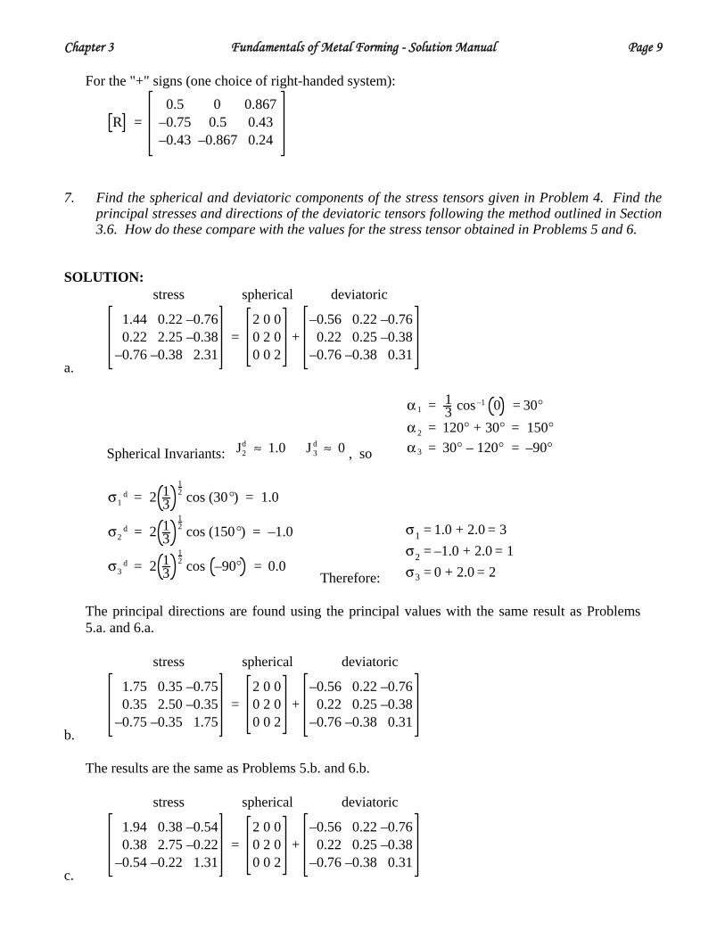
7. Find the spherical and deviatoric components of the stress tensors given in Problem 4. Find the
principal stresses and directions of the deviatoric tensors following the method outlined in Section 3.6. How do these compare with the values for the stress tensor obtained in Problems 5 and 6.
SOLUTION:
a.
stress spherical deviatoric
1.44 0.22 –0.760.22 2.25 –0.38
–0.76 –0.38 2.31=
2 0 00 2 00 0 2
+–0.56 0.22 –0.76
0.22 0.25 –0.38–0.76 –0.38 0.31
Spherical Invariants: , so J2d ≈ 1.0 J 3
d ≈ 0
α 1 = 13 cos–1 0 = 30°
α 2 = 120° + 30° = 150°α 3 = 30° – 120° = –90°
σ1
d = 2 13
12 cos (30°) = 1.0
σ2d = 2 1
312 cos (150°) = –1.0
σ3d = 2 1
312 cos –90° = 0.0
Therefore:
σ1 = 1.0 + 2.0 = 3σ2 = –1.0 + 2.0 = 1σ3 = 0 + 2.0 = 2
The principal directions are found using the principal values with the same result as Problems 5.a. and 6.a.
b.
stress spherical deviatoric
1.75 0.35 –0.750.35 2.50 –0.35
–0.75 –0.35 1.75=
2 0 00 2 00 0 2
+–0.56 0.22 –0.76
0.22 0.25 –0.38–0.76 –0.38 0.31
The results are the same as Problems 5.b. and 6.b.
c.
stress spherical deviatoric
1.94 0.38 –0.540.38 2.75 –0.22
–0.54 –0.22 1.31=
2 0 00 2 00 0 2
+–0.56 0.22 –0.76
0.22 0.25 –0.38–0.76 –0.38 0.31

Page 10 Fundamentals of Metal Forming - Solution Manual Chapter 3
The results are the same as Problems 5.c. and 6.c. 8. Find the spherical, deviatoric, principal deviatoric components, and principal directions of stress
for the following cases:
Uniaxial tension: σ11 = σ, other σ ij = 0
Simple shear: σ21 = σ12 = σ, other σ ij = 0
Balanced biaxial tension: σ11 = σ22 = σ, other σ ij = 0
Biaxial shear: σ13 = σ31 = σA, σ21 = σ12 = σB, other σij = 0
Tension and shear: σ11 = σt, σ13 = σ 31 = σs, other σij = 0
SOLUTION:
a. Uniaxial tension σ11 = σ, other σ ij = 0
,
stress spherical deviatoric
σ 0 0
0 0 0
0 0 0
=
σ3 0 0
0 σ3 0
0 0 σ3
+
2σ3 0 0
0 –σ3 0
0 0 –σ3
σ1
d =2σ3
σ2d = σ3
d = –σ3
m ↔ 1, 0, 0
n ↔ 0, 1, 0 (current axes are principal)
p ↔ 0, 0, 1
b. Simple shear σ12 = σ, other σ ij = 0
,
stress spherical deviatoric0 σ 0σ 0 00 0 0
=0 0 00 0 00 0 0
+0 σ 0σ 0 00 0 0
σ12d = σ21
d = σ, σ ijd = 0
m ↔ 12 , 1
2 , 0
n ↔ 0, 0, 1
p ↔ 12 , – 1
2 , 0

Chapter 3 Fundamentals of Metal Forming - Solution Manual Page 11
c. Balanced biaxial tension σ11 = σ22 = 0, other σ ij = 0
stress spherical deviatoric
σ 0 0
0 σ 0
0 0 0
=
2σ3 0 0
0 2σ3 0
0 0 2σ3
+
σ3 0 0
0 σ3 0
0 0 –2σ3
σ1d = σ2
d =σ3
σ3d = –
2σ3
m ↔ 1, 0, 0
n ↔ 0, 1, 0 (current axes are principal)
p ↔ 0, 0, 1
d. Biaxial shear σ13 = σ31 = σA, σ12 = σ21 = σB, other σ ij = 0
stress spherical deviatoric
0 σB σA
σB 0 0σA 0 0
=0 0 00 0 00 0 0
+0 σB σA
σB 0 0σA 0 0
σ1 = σB2 + σA
2
σ2 = 0
σ3 = σB2 + σA
2
m ↔ 1
2, σB
2 σB2 + σA
2, σA
2 σB2 + σA
2
n ↔ 0, σA
σA2 + σB
2, – σB
σA2 + σB
2
p ↔ – 12 , σB
2 σB2 + σA
2, σA
2 σB2 + σA
2
e. Tension and shear: σ11 = σt, σ13 = σ31 = σs, other σij = 0
stress spherical deviatoric
σ t 0 σ3
0 0 0σs 0 0
=
σ t3 0 00 σ t
3 00 0 σ t
3
+
2σ t3 0 σs
0 – σ t3 0
σs 0 – σ t3
σ1 =
σ t + σ t2 + 4 σs
2
2σ2 = 0
σ3 =σ t – σ t
2 + σs2
2

Page 12 Fundamentals of Metal Forming - Solution Manual Chapter 3
m ↔ σ s
D , 0, σ t – σ 1D , where D = σ t – σ1
2 + σ s2
12
n ↔ 0, 1, 0
p ↔ ±σ s
D′ , 0,σ t – σ2
D ′ , where D = σ t – σ22
+ σs2
12
(If σsσ t < 0, the minus sign is adopted for the components of p.) B. DEPTH PROBLEMS 9. The reciprocal theorem of Cauchy states that the stress vectors acting on two intersecting planes
have the following property:
s 1⋅ n2 = s 2⋅ n1 where si is the stress vector acting on a plane with normal ni. Show that this principle follows
from the symmetry of the stress tensor, or from the equilibrium condition directly. SOLUTION:
It is possible to prove the relationship by considering Cauchy's tetrahedron (Exercise 3.1), or by multiplying all of the required components and comparing the results. The shortest method is by writing the various terms in indicial notation.
Let n1 = n, n 2 = m, and s 1 = s and s 2 = t for simpler notation, then
s = σ n ↔ si = σ ij nj
t = σ m ↔ ti = σ ij mj
s ⋅ m = σ n⋅m or, s ⋅ m = si m i = σ ij n j mi
t ⋅ n = σ m n or t ⋅ n = ti ni = σ ij m jni
but, since we can rewrite σ ij = σ ji, σ ij n jmi = σ ij ni m j, so s ⋅ m = t ⋅ n. 10. Octahedral planes are ones which have normals forming equal angles with the three principal
axes. Find an expression for , the normal components of the stress vector on the octahedral plane in terms of a) principal stresses and b) arbitrary stress components.
Sn
SOLUTION:

Chapter 3 Fundamentals of Metal Forming - Solution Manual Page 13
n
x1
x3
x2
a. In principal axes, as show in the figure above,
σ =σ1 0 00 σ2 00 0 σ3
, and n =
131313
Therefore:
Sn = n⋅S⋅n = 13
13
13
σ1 0 00 σ 2 00 0 σ3
131313
= 13 (σ1 +σ 2 + σ3) p = 1
3 J1 (Eq. 2.38)
where J1 is the first stress invariant.
b. Since we know that this quantity is invariant to the choice of coordinate system orientation, the expression in an arbitrary cartesian system is
Sn = p = 13 J1 = 1
3 (σ11 +σ22 + σ33)
11. Show that the tangential component of the stress vector on the octahedral planes (i.e. the shear
component) is equal to
23
J2'
12
, where J is the second invariant of the deviatoric stress tensor. 2' SOLUTION:
As shown in Problem 10., the normal component on an octahedral plane is
SN =
13
σ1 + σ2 + σ3
The tangential component may be found from the relationship SN
2 + S T2 = S ⋅ S = (σ ⋅ n) ⋅ (σ ⋅ n), or
ST2 = (σ ⋅ n) ⋅ (σ ⋅ n) – SN
2 = 13 σ1
2 + σ22 + σ3
2 – 19 σ1 + σ2 + σ3
2
9 ST
2 = 2 σ12 + 2 σ2
2 + 2 σ32 – 2 σ1σ2 – 2 σ1σ3 – 2 σ2σ3 = 6 J2
Page 14 Fundamentals of Metal Forming - Solution Manual Chapter 3
So,
ST = 23 J2
′12
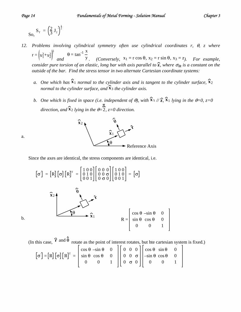
12. Problems involving cylindrical symmetry often use cylindrical coordinates r, θ, z where
r = x12+x2
212
and
θ = tan-1 x
y . (Conversely, x1 = r cos θ, x2 = r sin θ, x3 = z). For example, consider pure torsion of an elastic, long bar with axis parallel to z, where σθz is a constant on the outside of the bar. Find the stress tensor in two alternate Cartesian coordinate systems:
a. One which has x1 normal to the cylinder axis and is tangent to the cylinder surface, x2
normal to the cylinder surface, and x3 the cylinder axis. b. One which is fixed in space (i.e. independent of θ), with x3 // z, x1 lying in the θ=0, z=0
direction, and x2 lying in the θ=π2, z=0 direction.
a.
x1
x2
Reference Axis
rθ
θ
Since the axes are identical, the stress components are identical, i.e.
σ′ = R σ R T =
1 0 00 1 00 0 1
0 0 00 0 σ0 σ 0
1 0 00 1 00 0 1
= σ
b. x1
x2 rθ
θ
R =cos θ –sin θ 0sin θ cos θ 0
0 0 1
(In this case, r and θ rotate as the point of interest rotates, but hte cartesian system is fixed.)
σ′ = R σ R T =cos θ –sin θ 0sin θ cos θ 0
0 0 1
0 0 00 0 σ0 σ 0
cos θ sin θ 0–sin θ cos θ 0
0 0 1

Chapter 3 Fundamentals of Metal Forming - Solution Manual Page 15
=
cos θ –sin θ 0
sin θ cos θ 0
0 0 1
0 0 0
0 0 σ
σ –sin θ σcos θ 0
σ′ =0 0 –σ sin θ0 0 σ cos θ
–σ sin θ σ cos θ 0
(fixed Cartesian system) 13. Show that if two roots of the characteristic equation are identical (i.e. degenerate), then any
direction normal to the other principal direction (i.e. the one corresponding to the non-identical root) is a principal direction. Show that if all three roots are identical, all directions are principal.
SOLUTION: a. Assume that the characteristic equation is of the form:
λ – σo λ – σ1
2 = 0 , where σ is a degenerate root. The stress components in the principal axes are 1
σ1 0 00 σ1 00 0 σo
, where is the principal stress in the (3rd principal) direction. A general rotation of coordinate system about the axis may be written as follows:
σo x3′
x3′
σ =cos θ sin θ 0–sin θ cos θ 0
0 0 1
σ1 0 00 σ1 00 0 σo
cos θ –sin θ 0sin θ cos θ 0
0 0 1=
=
σ1 cos2 θ + sin2 θ σ1 –sin θ cos θ + sin θ cos θ 0
σ1 sin θ cos θ – sin θ cos θ σ1 sin2 θ + cos2 θ 0
0 0 σo
=

Page 16 Fundamentals of Metal Forming - Solution Manual Chapter 3
σ =σ1 0 00 σ1 00 0 σo
for any direction normal to x3′
b. If all three roots are degenerate, there are many ways to show that any direction is equivalent. The derivation in Part a. can be done for , or one can note that all three roots being equivalent is the same as the spherical component (i.e. hydrostatic pressure or tension).
σ1 = σo
14. It is often convenient to replace one set of forces with another, statically-equivalent set. For
example, consider a triangular element of material (assume unit depth normal to the triangle) which is assumed to be a small enough piece of a body to feel only a homogeneous stress, σij (i,j=1,2, assuming that σi3=0, where x3 is normal to the triangle). Use a simple, physically-motivated procedure to replace σij by three forces, f1, f2, f3 acting at the three corners of the triangle. Consider the force transmitted by each face.
SOLUTION:
Consider a triangle with normals defined to each side with a magnitude equal to the length of the side. (For unit depth of the sides in three dimensions, these are area vectors corresponding to the sides.)
1
3
b
c
A
B
C
σ
where:A = aB = bC = c
A, B, C are deduced from a, b, and c by a rotation of -90o, therefore since a + b + c = 0, A + B + C = 0. The forces acting on the planes A, B, and C are fA = σ A, fB = σ B, fC = σ C
and fA + fB + fC = σ A + B + C = 0 because A+ B + C = 0. To assign these forces to the vertices, let's use the unweighted average (although other choices might make more physical sense) of the forces on the connected sides:
f1 = 12 fA + fC = 1
2 σ A+ C
f2 = 12 fA + fB = 1
2 σ A+ B
f3 = 12 fB + fC = 1
2 σ B + C
15. Physically, why can the entire material loading at a point be reduced to three orthogonal force
intensities passing through the point? Why do the shear components disappear along these directions?
SOLUTION:

Chapter 3 Fundamentals of Metal Forming - Solution Manual Page 17
For simplicity, let's consider a two-dimensional situation first. Similar to Figure 3.1, imagine making an arbitrary mathematical cut as shown in part (a) of the figure below. We can find the force acting on one of the cut faces required to maintain equilibrium, part (b). (The opposite force is required on the other cut face by equilibrium.) Then, glue the first cut back togehther and using the direction of the force as a guide, make another cut, this one perpendicular to the force observed on the first cut. Find the new force required for equilibrium and, if necessary, make another cut perpendicular to the new force. Continue until the current cut and current force are perpendicular, part (c). If we now relax the forces on the cut plane (and any external forces required to maintain equilibrium as the cut face is unloaded), can we be assured that the material is completely unloaded? No, because the direction parallel to the cut face (grey arrow in part (c)) is unaffected by the cut and therefore we have no information about it. Therefore, make a cut perpendicular to the final first cut and the force required by equilibrium will by necessity be perpendicular to the first force, part (d). This simple thought exercise demonstrates why there are only two independent force intensities passing through a point in a two-dimensional body, and why they must be perpendicular. To extend the exercise to three dimensions, follow precisely the same procedure. Once the first plane and normal force are found, there remain two perpendicular planes which must have only normal forces acting on them.
(a) (b) (c) (d) Although opposite to the usual derivation, it would be possible to derive the symmetry of the stress tensor by first noting that this result requires the existence the three perpendicular principal directions and that any rotation of axes from this principal set must produce a symmetric and real set of tensor components.
16. The two sets of components presented below correspond to the identical stress tensor, as measured
in two coordinate systems, x1, x2, x3, and x1', x2', x3' . Find the rotation matrix to transform components from the x i system to the x i' system, and vice versa. (Hint: First find the rotations to the common, principal coordinate systems.)
σ =1.000 1.730 1.0001.730 0.750 0.4331.000 0.433 0.250
σ′ =0.500 1.414 0.5001.414 1.000 1.4140.500 1.414 0.500
SOLUTION:
σ′ = R σ R T

Page 18 Fundamentals of Metal Forming - Solution Manual Chapter 3
Define rotation matrices R1 and R2 such that
σprincipal = R1 σ R1
T
σprincipal = R2 σ′ R2
T
Then, we can find [R] in terms of R1 and R2
σprincipal = R1 σ R1
T = R2 σ1′ R2
T
R2
T R1 σ R1T R2 = R2
T R2 σ1′ R2
T R2 = σ1′
Therefore: R = R2
T R1 , R T = R1T R2
We find R1 and R2 as usual:
σ =1.0 1.73 1.0
1.73 0.75 0.4331.0 0.433 0.25
⇒σ1 = 3σ2 = 0σ 3 = –1
⇒n ↔ (0.707, 0.612, 0.36)m ↔ (0.0, 0.50, –0.866)
p ↔ (– 0.707, 0.61, 0.36)
So,
R1 =0.707 0.61 0.360.0 0.50 –0.866
–0.707 0.61 0.36
σ′ =0.50 1.414 0.501.414 1.0 1.4140.50 1.414 0.50
⇒σ1 = 3σ2 = 0σ1 = –1
⇒n ↔ (0.50, 0.707, 0.50)m ↔ (0.707, 0, –0.707)p ↔ (– 0.50, 0.707, –0.50)
R2 =0.50 0.707 0.500.707 0.0 –0.707–0.50 0.707 –0.50
Therefore:
R R2T R1 =
0.71 0.36 –0.610 0.86 0.51
0.71 –0.36 0.61
17. Imagine that we define a new measure of stress, [S], as a matrix of components relating force
components to area components, but that the force components are defined in two ways: 1. in terms of a different coordinate system than the area components, or 2. the are transformed according to a fixed linear operation to represent a new vector in the same coordinate system. a) Is [S][ symmetric? b) According to these two definitions, does [S] represent the components of tensor?
SOLUTION:
In either of cases 1 or 2, we note that the new force components (let us call these components gi) may be obtained from the standard force components fi as follows (note that by "standard" we mean the components of a force as normally defined in the same coordinate system used to

Chapter 3 Fundamentals of Metal Forming - Solution Manual Page 19
express vector area components):
g = L f , where [L] is a linear operator (rotation or other transformation matrix)
a. The definition of [S] follows from the expression of [g]:
g = s a ⇒ L f = s a , ⇒ f = L – 1 s a
σ
∴ σ = L – 1 s , or s = L σ Since [L] is a general, non-symmetric matrix, [s] is in general not symmetric.
b. In order to examine how the new stress measure [S] transforms, let's imagine that we want to
express [S] in a new coordinate system: x ′ = R x . In the new coordinate system, our
definitions will be expressed as follows:
g ′ = S′ a ′
, where a ′ = R a
The central question, the one that differentiates Case I from Case II, is: What is the meaning of g ′
?
Case 1 - According to the definition of Case 1, g ′
is found in the new coordinate system by applying the fixed linear operator, [L], to the components of [f] in the new coordinate system:
g ′ = L f ′ = L R f ,
once this expression for g ′
is found, we can find how S and S ′
are related:
g ′ = L R f = S ′ a ′ = S ′ R a
f = R T L –1 S′ R a , but note that f = L –1 g
, so
g = L R T L –1 S′ R a
S , and therefore
S = L R T L –1 S′ R , or S′ = L –1 R L S R T
Clearly this last expression is not the proper transformation for tensor components, so [S] defined as in Case 1 does not represent tensor components.
Case 2 - According to the definition of Case 2, g ′
is found in the new coordinate system by simply transforming the compents of g as any other vector in the original coordinate system, i.e.
g ′ = R g ,

Page 20 Fundamentals of Metal Forming - Solution Manual Chapter 3
once we have this expression for g ′
, we proceed as before to find the relationship between S
and S ′
:
g ′ = R g = S ′ a ′ = S′ R a
g = R T S′ R a
S , and therefore
S = R T S ′ R , or S′ = R S R T
This last expression is precisely the transformation for tensor components, so [S] defined in Case 2 does represent tensor components. Put more simply, S defined according to Case 2 is a proper tensor. In fact, representation of stress in this manner is convenient in some cases, where the force or area vectors are rotated to correspond to deformed or undeformed states in a material.
CHAPTER 4 - PROBLEM SOLUTIONS
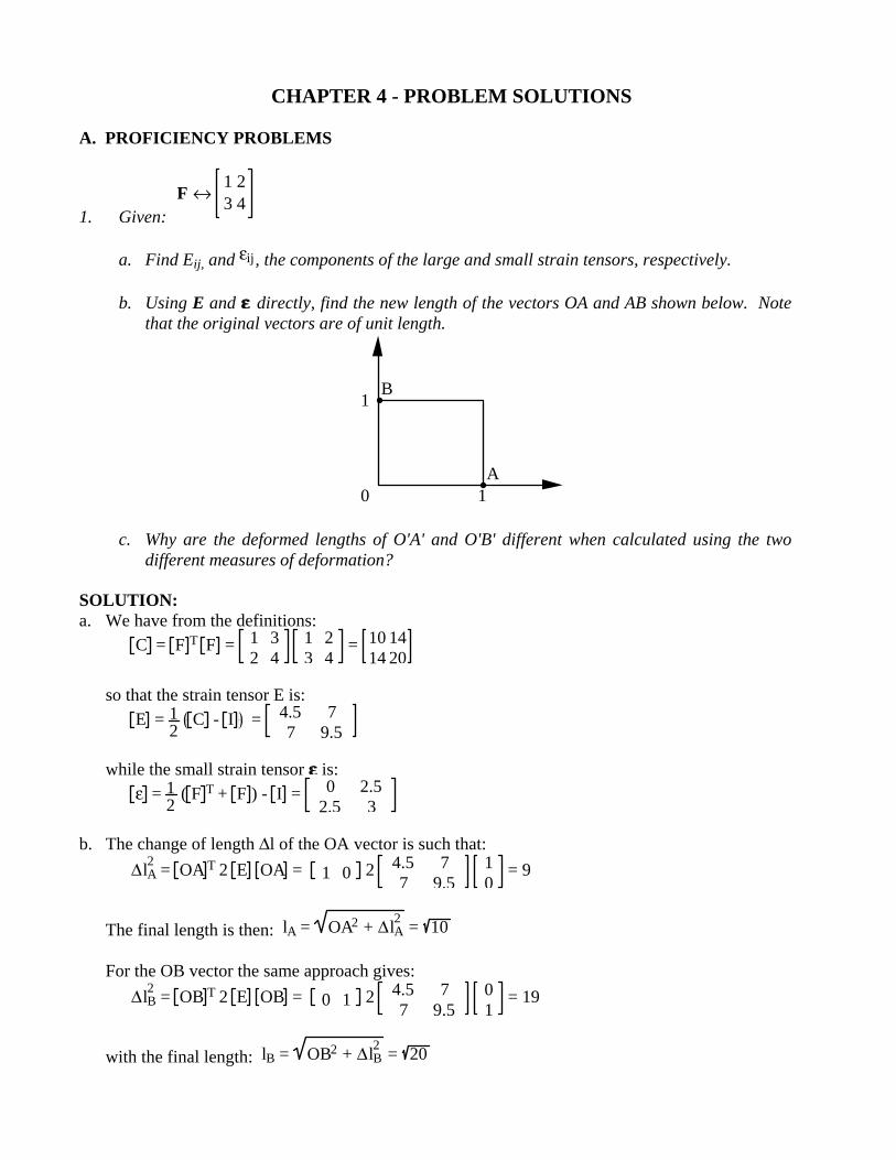
A. PROFICIENCY PROBLEMS
1. Given:
F ↔
1 23 4
a. Find Eij, and ε , the components of the large and small strain tensors, respectively. ij
b. Using E and ε ε directly, find the new length of the vectors OA and AB shown below. Note
that the original vectors are of unit length.
0 1
1
A
B
c. Why are the deformed lengths of O'A' and O'B' different when calculated using the two different measures of deformation?
SOLUTION: a. We have from the definitions:
C = F T F = 1 3
2 4 1 2
3 4 = 10 14
14 20 so that the strain tensor E is:
E = 1
2 C - I = 4.5 7
7 9.5 while the small strain tensor ε ε is:
ε = 1
2 ( F T + F ) - I = 0 2.5
2.5 3 b. The change of length Δl of the OA vector is such that:
ΔlA
2 = OA T 2 E OA = 1 0 2 4.5 77 9.5
10
= 9
The final length is then: lA = OA2 + ΔlA2 = 10
For the OB vector the same approach gives:
ΔlB
2 = OB T 2 E OB = 0 1 2 4.5 77 9.5
01
= 19
with the final length: lB = OB2 + ΔlB2 = 20
Page 2 Fundamentals of Metal Forming - Solution Manual Chapter 4
With the small strain tensor [ε] the new lengths are:
lA2 = 1 + OA T 2 ε OA = 1 + 1 0 2 0 2.5
2.5 010 = 1
and
lB2 = 1 + OB T 2 ε OB = 1 + 0 1 2 0 2.5
2.5 301 = 7
c. The results are quite different when we use the two strain measures: in fact the use of the [ε] tensor is not valid here as the strain components are not much less than 1, as required for accuracy.
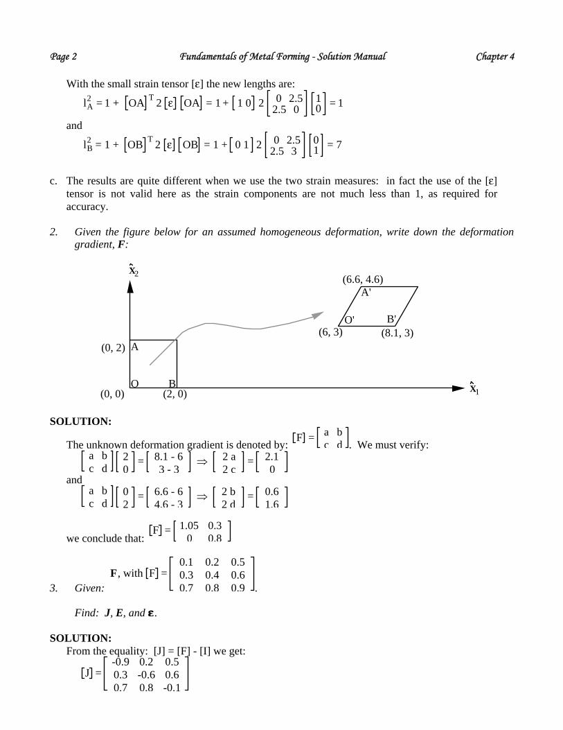
2. Given the figure below for an assumed homogeneous deformation, write down the deformation gradient, F:
A'
B'O'
(6.6, 4.6)
(6, 3) (8.1, 3)A
BO
(0, 2)
(0, 0) (2, 0)
X2
X1
SOLUTION:
The unknown deformation gradient is denoted by: F = a b
c d . We must verify:
a bc d
20
= 8.1 - 63 - 3
⇒ 2 a2 c
= 2.10
and
a bc d
02
= 6.6 - 64.6 - 3
⇒ 2 b2 d
= 0.61.6
we conclude that: F = 1.05 0.3
0 0.8
3. Given: F, with F =
0.1 0.2 0.50.3 0.4 0.60.7 0.8 0.9 .
Find: J, E, and ε ε.
SOLUTION:
From the equality: [J] = [F] - [I] we get:
J =
-0.9 0.2 0.50.3 -0.6 0.60.7 0.8 -0.1

Chapter 4 Fundamentals of Metal Forming - Solution Manual Page 3
The strain tensor [E] is writen:
E = 12
F T F - I = 12
0.1 0.3 0.70.2 0.4 0.80.5 0.6 0.9
0.1 0.2 0.50.3 0.4 0.60.7 0.8 0.9
- 1.0 0 00 1.0 00 0 1.0
= 1200
1+3*3+7*7-100 2+3*4+7*8 5+3*6+7*9
sym 2*2+4*4+8*8-100 2*5+4*6+8*9sym sym 5*5+6*6+9*9-100
= -0.205 0.35 0.430.35 -0.08 0.530.43 0.53 0.21
The small strain tensor is:
ε = 1
2
-0.9 0.2 0.50.3 -0.6 0.60.7 0.8 -0.1
+ -0.9 0.3 0.70.2 -0.6 0.80.5 0.6 -0.1
= -0.9 0.25 0.60.25 -0.6 0.70.6 0.7 -0.1
4. As shown below, a point in a continuum (O) moves to a new point (O') as shown.
x2
A
B1.5O
1.5
x1
O' (4,2)
B'
A'
a. Find the new points A' and B', assuming homogeneous deformation for the following two cases:
F ↔ 1 2
3 4 , J ↔ 2 1
4 3 b. For each deformation, find E the large strain tensor.
SOLUTION:
By definition of the deformation gradient (when there is an homogeneous deformation), we obtain for the first case:
OA → O′A′ with: O′A′ = F OA = 1 2
3 4 0
1.5 = 3
6
and OB → O′B′ with: O′B′ = F OB = 1 2
3 4 1.5
0 = 1.5
4.5
Page 4 Fundamentals of Metal Forming - Solution Manual Chapter 4
so that:
OA′ = OO′ + O′A′ = 42
+ 36
= 78
OB′ = OO′ + O′B′ = 42
+ 1.54.5
= 5.56.5
For the second case we have first: F = J + I = 3 1
4 4 The transformation verifies:
OA → O′A′ with: O′A′ = F OA = 3 1
4 4 0
1.5 = 1.5
6
and OB → O′B′ with: O′B′ = F OB = 3 1
4 4 1.5
0 = 4.5
6
so that
OA′ = OO′ + O′A′ = 4
2 + 1.56 = 5.5
8
OB′ = OO′ + O′B′ = 42 + 4.5
6.0 = 8.58
b. For the first case we have
E = 1
2 F T F - I = 1
2 1 3
2 4 1 2
3 4 - 1 0
0 1 = 4.5 7
7 9.5 and for the second case
E = 1
2 J + J T + J T J = 12
2 14 3 + 2 4
1 3 + 2 41 3
2 14 3 = 12 9.5
9.5 8.0
5. Imagine that a line segment OP is embedded in a material which is deformed to a new state. The
line segment becomes O'P' after deformation, as shown below.
O
O'
P(2, 1)
P'ˆ x 2
ˆ x 1
a. Find the vector components of O'P' :
F ↔ 1 2
3 4
b. Find the length of O'P' if:

Chapter 4 Fundamentals of Metal Forming - Solution Manual Page 5
C = 1 3
3 2
c. Find the components of OP if:
J = 0 2
3 3 SOLUTION: a. If the deformation is homogeneous we can write:
OP → O′P′ such that: O′P′ = F OP = 1 2
3 4 2
1 = 4
10
b. According to Eq. 4.19:
O′P′2 = OP T C OP = 2 1 1 3
3 2 2
1 = 2 1 5
8 = 18
the final length is then: O′P′ = 18 ≅ 4.24
c. From [J] we deduce:
OP → O′P′ such that: O′P′ = J + I OP = 1 2
3 4 2
1 = 4
10
6. A homogeneous deformation is imposed in the plane of the sheet. Two lines painted on the surface move as shown below, with coordinates measured as shown:
(1.8, 2.1)
(2, 1.5)
(1, 1)
Before After
(3.1, 3.3)
(3, 2)(4.1, 1.9)
1̂ x
ˆ x 2ˆ x 2
1̂ x
a. Find F, the deformation gradient. b. Starting with F, find C, E, and ε ε. c. Find the principal strains and axes of E.
SOLUTION: a. The method is similar to that used for Problem 2. We express that the deformation gradient
applied to the two vectors (as rows) gives their transformed coordinates:
a bc d
1 0.80.5 1.1
= 1.1 0.1-0.1 1.3

Page 6 Fundamentals of Metal Forming - Solution Manual Chapter 4
The best method is to invert the matrix on the left hand side:
1 0.8
0.5 1.1-1
= 10.7
1.1 -0.8-0.5 1
so that the unknown deformation gradient is:
a bc d
= 1.1 0.1-0.1 1.3
10.7
1.1 -0.8-0.5 1
= 10.7
1.16 -0.78-0.76 1.38
≅ 1.66 -1.11-1.09 1.97
b. The usual tensors are computed:
C = 1
0.7 1.16 -0.76
-0.78 1.38 1
0.7 1.16 -0.78
-0.76 1.38 = 1
0.49 1.9232 -1.9536
-1.9536 2.5128 ≅ 3.92 -3.99
-3.99 5.13
E = 1
2 3.92-1 -3.99
-3.99 5.13-1 = 1.46 -2
-2 2.07
ε = 1
2 1.66-1 -1.11
-1.09 1.97-1 + 1.66-1 -1.09
-1.11 1.97-1 = 0.66 -1.10
-1.10 0.97 (But again in this case the small strain tensor has no precise meaning, as its components are not small with respect to 1).
c. The principal strains are solutions of the eigenvalue problem:
1.46-λ -2
-2 2.07-λ = 0, or (1.46- λ) (2.07-λ) - 4 = 0
which is also: λ2 - 3.53 λ - 0.98 = 0 with solutions E1 = -0.26 and E2 = 3.79 The principal axes v are such that their components verify: 1 and v 2
(1.46 + 0.26) v11 - 2 v21 = 0 ⇒ v1 = 0.760.65
(1.46 - 3.79) v12 - 2 v22 = 0 ⇒ v2 = -0.650.76
7. At time t, the position of a material particle initially at (X1, X2, X3) is
x1 = X1 + a X2 x2 = X2 + a X1 x3 = X3
Obtain the unit elongation (i. e. change in length per unit initial length) of an element initially in the direction of x1 + x2.
SOLUTION:
Chapter 4 Fundamentals of Metal Forming - Solution Manual Page 7
The deformation gradient is here: F = Žx
ŽX , F =
1 a 0a 1 00 0 1
and the Cauchy strain tensor is immediately deduced:
C = 1+a2 2a 0
2a 1+a2 0
0 0 1
The initial unit vector is:
dS ↔
12120
The length of the final corresponding vector verifies:
ds2 = dS T C dS = 12
12
0 dS 1+a2 2a 0
2a 1+a2 0
0 0 1
12120
dS = (1 + a)2 dS2
so that ds = (1 + a) dS and the unit elongation is: E = a.
8. Take fixed right handed axes x1, x2, x3. Write down the deformation gradient matrix,
∂Xi∂xj , for the
deformation of a body from x to X for
a. right handed rotation of 45o about x1. b. Left handed rotation of 45o about x2. c. Stretch by a stretch ratio of 2 in the x3 direction.
d. Stretch by a stretch ratio of 12 in the x2 direction.
e. Right handed rotation of 90o about x3.
Find the total deformation matrix for these motions carried out sequentially. Using this result,
check the final volume ratio.
SOLUTION:
The deformation gradients are computed at each step:

Page 8 Fundamentals of Metal Forming - Solution Manual Chapter 4
Fa =
1 0 0
0 12
- 12
0 12
12
, Fb =
12
0 - 12
0 1 0
12
0 12
Fc =
1 0 00 1 00 0 2
, Fd =1 0 00 1/2 00 0 1
, Fe =0 -1 01 0 00 0 1
The combined transformation has a deformation gradient:
F = Fe Fd Fc Fb Fa =
0 - 24
24
22
- 12
- 12
2 1 1
The Cauchy strain tensor is then evaluated:
C =2.5 1.06 1.06
1.06 1.38 1.121.06 1.12 1.38
We see immediately that: C = 1, i. e. the deformation takes place with no volume change.
9. From the following mapping, find C, U, and R:
x1x2x3
= 2 0 00 3 40 4 -3
X1X2X3
Check whether this is a permissible deformation in a continuous body. SOLUTION:
The Cauchy strain tensor is first calculated by:
C =
2 0 00 3 40 4 -3
2 0 00 3 40 4 -3
= 4 0 00 25 00 0 25
The polar decomposition is written: [F] = [R] [U]; with [U]2 = [C] we deduce:
U = 2 0 00 5 00 0 5
and R = F U -1 = 2 0 00 3 40 4 -3
12
0 0
0 15
0
0 0 15
=
1 0 0
0 35
45
0 45
- 35
But we see that R = - 1 so that [R] is not a rotation, but rather an inversion.
Chapter 4 Fundamentals of Metal Forming - Solution Manual Page 9
10. Check the compatibility of the following strain components:
ε ε ↔ x1+x2 x1+2x2 0x1+2x2 x1+x2 0
0 0 x3
ε ε ↔ x12 x12+x22 x2x3
x12+x22 x22 0
x2x3 0 0
SOLUTION:
From the strain tensor:
ε =x1+x2 x1+2x2 0
x1+2x2 x1+x2 00 0 x3
the components of which are first order polynomials, we see that: (see also Problem 15)
Ž2εii
Žxj2
+ Ž2εjj
Žxi2
= 2 Ž2εij
Žxi ∂xj = 0
so that the field is compatible.
The second strain tensor is:
ε = x12 x12+x22 x2x3
x12+x22 x22 0
x2x3 0 0
we observe that:
Ž2ε2
Žxj2
+ Ž2εjj
Žxi2
= 2 Ž2εij
Žx1 ∂x2 = 0
Ž2ε22
Žx32
+ Ž2ε33
Žx22
= 0 = 2 Ž2ε23
Žx2 ∂x3
Ž2ε33
Žx12
+ Ž2ε11
Žx32
= 0 = 2 Ž2ε13
Žx1 ∂x3 So that this tensor field is also compatible.
B. DEPTH PROBLEMS 11. Consider the extension of an arbitrary small line element AB. Start by examining how (A'B')2 is
related to (AB)2 using the small extensional strain along that direction, en. Show that for small strains and displacements, rotations do not cause extension, i.e. if extensions are zero, strains are zero.
SOLUTION:
We put: AB = a dl, where a is a unit vector, and write Eq. 4.18 in the form:

Page 10 Fundamentals of Metal Forming - Solution Manual Chapter 4
A′B′2 = (a dl)T C a dl = dl2 aT(I + J)T (I + J) a = AB2 aT (I + JT + J + JT J) a Using the small strain approximation we obtain:
A′B′2 ≅ AB2 aT (I + JT + J) a = AB2 aT (I + 2 ε ε) a As the components of the strain tensor are small with respect to unity we can also write: A′B′ ≅ AB (1 + 2 aT ε ε a)1/2 ≅ AB (1 + aT ε ε a) If we have only an extension en in the x1 direction, the previous equation becomes:
A′B′ ≅ AB (1 + en) (where we used a =
100
)
If there is zero extension in any direction we have: A′B′ = AB = AB (1 + aT ε ε a) for any a, that is also: aT ε ε a = 0 If a is a principal direction, the above equality shows that the corresponding principal strain must be zero, so that we come to the conclusion that the strain tensor must be null.
12. In sheet forming, one often measures strains from a grid on the sheet surface. Then, one can plot these strains as a function of the original length along an originally straight line:
������
Original LineStrain
Original Position
����
Die Die
����PUNCH
As shown in the second figure (for a simple forming operation), this originally straight line is
curved and stretched. If the edges of the sheet do not move (stretch boundary conditions), develop a rule that the
measured strain distribution must follow. Consider that the original sheet length lo becomes l at some later time.
SOLUTION:
We consider the strain εl or e1 (true or engineering definition) corresponding to the elongation in the initial direction of the line. A small vector dl0 on the initial line will be transformed into a

Chapter 4 Fundamentals of Metal Forming - Solution Manual Page 11
small vector dl so that its new length verifies: dl = exp( . Therefore the final length of the line will be:
εl) dl0 = (1 + e1) dl0
l = exp(εl) dl0
0
l0
= (1 + e1) dl00
l0
13. Consider a 1" square of material deformed in the following ways:
0 3
2
dx1
dx2
a) 0
32 dx1dx2
b)
30°
0 3
2dx1
dx2
c)
3
0
32 dx 1
dx 2 45°
d)
0 1
1
dx1
dx2
Find F for each case. Find C and E. Find the principal values and directions of E. Find the material principal directions after deformation. Which of these cases (a-d) are mechanically the same under isotropic conditions? Under
general anisotropy? SOLUTION:
a. We have: F = 3 0
0 2 , C = 9 0
0 4 , E = 4 0
0 3/2 The principal strains are obviously: E , the principal axes and the material axes after deformation are the ox1 and ox2 axes.
1 = 3/2, E2 = 4
b. The new vectors are projected on the ox1 and ox2 axes so that we have:
F = 3 3/2 -1
3/2 3 , C = 3 3/2 3/2
-1 3 3 3/2 -1
3/2 3 = 9 0
0 4 , E = 4 0
0 3/2 The remaining is the same as case a.
c. F = -3 0
0 -2 , C = 9 0
0 4 , E = 4 0
0 3/2
Page 12 Fundamentals of Metal Forming - Solution Manual Chapter 4
The remaining is the same as case a.
d. F = 3 2/2 - 2
3 2/2 2 , C = 3 2/23 2/2
- 2 2 3 2/2 - 23 2/2 2
= 9 00 4
, E = 4 00 3/2
The remaining is the same as case a. For isotropic materials the four cases a-d are equivalent by definition, as a rotation has no effect on the material properties. Under general anisotropy case a is equivalent to the undeformed configuration (if the deformation does not introduce any change in the anisotropic coefficients), while cases b, c, d correspond to rotations of 30°; 180° and 45° respectively, and the material properties will be rotated by the same rotation.
14. Given that C = 1 0
0 2 , find F when
a. the principal material axes do not rotate, and
b. the principal material axes rotate by 30o counterclockwise. Express your answers in the original coordinate system.
SOLUTION: a. We use the polar decomposition: F = RU, if there is no rotation, then R = I, F = U is symmetric
and C = FF so that here F is easily computed:
F = U = 1 0
0 2
b. The rotation matrix is:
R = 32
- 12
12
32
The [U] stretch tensor is the same and the deformation gradient is:
F = R U = 32
- 12
12
32
1 0
0 2 =
32
- 22
12
62
15. Derive a set of compatibility equations corresponding to Eq. 4.52 for the three-dimensional case. SOLUTION:
A non diagonal (small) strain component is calculated according to:
εij = 1
2 (ŽUi
Žxj +
ŽUjŽxi
) for i ° j
so that we obtain:

Chapter 4 Fundamentals of Metal Forming - Solution Manual Page 13
2
Ž2εijŽxi Žxj
= Ž3Ui
Žxi Žxj2 +
Ž3Uj
Žxi2 Žxj
for i ° j
which is also, with the definition of the diagonal terms (without summation on i and j):
2
Ž2εijŽxi Žxj
= Ž2εii
Žxj2
+ Ž2εjj
Žxi2
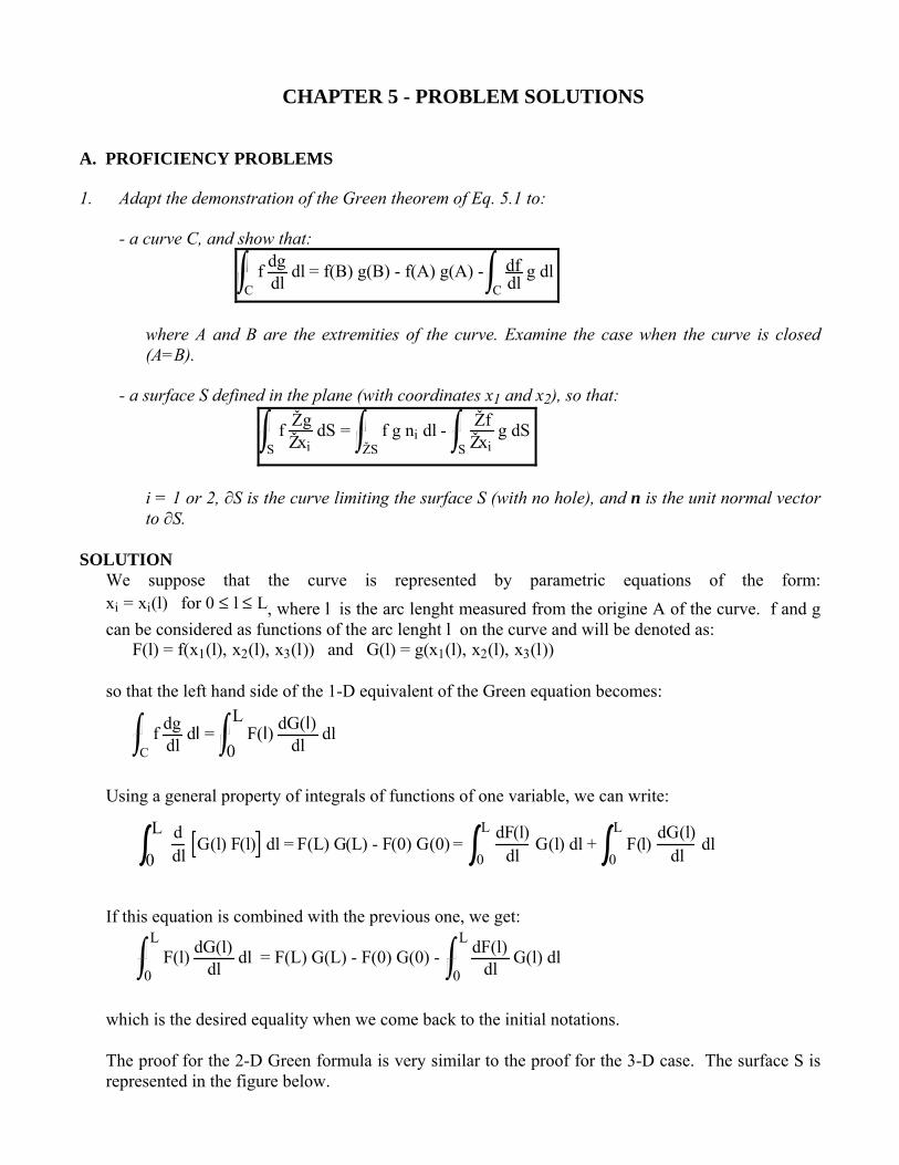
CHAPTER 5 - PROBLEM SOLUTIONS A. PROFICIENCY PROBLEMS 1. Adapt the demonstration of the Green theorem of Eq. 5.1 to:
- a curve C, and show that:
f dg
dl dl
C = f(B) g(B) - f(A) g(A) - df
dlg dl
C where A and B are the extremities of the curve. Examine the case when the curve is closed
(A=B). - a surface S defined in the plane (with coordinates x1 and x2), so that:
f ŽgŽxi
dSS
= f g ni dlŽS
- ŽfŽxi
g dS S
i = 1 or 2, ∂S is the curve limiting the surface S (with no hole), and n is the unit normal vector
to ∂S.
SOLUTION We suppose that the curve is represented by parametric equations of the form:
, where l is the arc lenght measured from the origine A of the curve. f and g can be considered as functions of the arc lenght l on the curve and will be denoted as: xi = xi(l) for 0 ≤ l ≤ L
F(l) = f(x1(l), x2(l), x3(l)) and G(l) = g(x1(l), x2(l), x3(l)) so that the left hand side of the 1-D equivalent of the Green equation becomes:
f dg
dl dl
C = F(l) dG(l)
dl dl
0
L
Using a general property of integrals of functions of one variable, we can write:
ddl
G(l) F(l) dl0
L= F(L) G(L) - F(0) G(0) =
dF(l)dl
G(l) dl0
L+ F(l)
dG(l)dl
dl0
L
If this equation is combined with the previous one, we get:
F(l) dG(l)
dl dl
0
L = F(L) G(L) - F(0) G(0) - dF(l)
dlG(l) dl
0
L
which is the desired equality when we come back to the initial notations. The proof for the 2-D Green formula is very similar to the proof for the 3-D case. The surface S is represented in the figure below.

Page 2 Fundamentals of Metal Forming - Solution Manual Chapter 5
x2
x1xA xB
S
ŽSU
ŽSL
The boundary of S is divided into an upper part ∂ΩU, and a lower part ∂ΩL the equations of which are respectively: x2 = hU(x1) ; x2 = hL(x1)
Using these notations, we can write:
f ŽgŽx2
dSΩ
= f ŽgŽx2
dx2hL(x1)
hU(x1) dx1
xA
xB
The above equation is transformed in a similar way as Eq. 5.3 so that:
f ŽgŽx2
dx2hL
hU
= fU gU - fL gL - ŽfŽx2
g dx2hL
hU
This equation is now integrated with respect to x1:
f ŽgŽx2
dSS
= fU gU - fL gL dx1xA
xB
- ŽfŽx2
g dx2hL
hU
dx1
xA
xB
In a way similar to Eqs. 5.3a and 5.3b, the component nU2 of the normal to ∂ΩU is such that dx1 = nU2 dl and an analogous equation for the lower part of the boundary. Then we get:
fU gU - fL gL dx1
xA
xB
= fU gU nU2 dlxA
xB
- fL gL nL2 dlxA
xB
= fg dl ∂S
When this last result is put into the previous equation we obtain the 2-D form of the Green theorem:
f ŽgŽx2
dSS
= fg n2 dl∂S
- ŽfŽx2
g dS S
2. Apply the 2-D form of the Green theorem (see problem 1) to the functions f = x1 + x2 and g = x1 - x2 in the square domain [0,1]2, for i = 1 and for i = 2. Compute directly the integrals and verify the Green theorem on this specific example.

Chapter 5 Fundamentals of Metal Forming - Solution Manual Page 3 SOLUTION:
We must show that the following equality holds:
f ŽgŽx2
dx20
1 dx1
0
1
= fg n2 dl∂S
- ŽfŽx2
g dx20
1 dx1
0
1
The first integral in the above equation is computed according to:
0
1(x1 + x2) (-1) dx20
1dx1 = 01- x1x2 +
x12
2 x2=0
x2=1
dx1 = - (x1 +12
) dx10
1= -
x12
2+
x1
2 0
1
= -1
On the boundary of the square, the n2 component is non-zero only on the segments corresponding to x2 = 0 or 1, so that the second integral is:
fg n2 dl
∂S = (x1 + 1) (x1 - 1) dx1
0
1 - x1
2 dx10
1 = -1
Finally the third integral is written:
(x1 - x2) dx20
1dx1
0
1
= x1x2 -x1
2
2 x2=0
x2=1
dx1
0
1
= (x1 -12
) dx10
1=
x12
2-
x1
2 0
1
= 0
Using the numerical values of the three contributions allows verification of the Green theorem for this particular case.
3. A 2-D velocity field is given by the expressions:
v1 = a x12 + 2 b x1 x2 + c x1 x2
v2 = a′x12 + 2 b′x1 x2 + c′x1 x2
depending on the 6 parameters a, b, c, a', b', c'. Determine the relations the parameters must
satisfy in order that the velocity field is incompressible. Keeping these relations in mind, show directly that the material flow through the hatched unit triangle pictured below is equal to zero.

Page 4 Fundamentals of Metal Forming - Solution Manual Chapter 5
O x1
x2
1
1 SOLUTION:
The partial derivatives are first evaluated by:
Žv1Žx1
= 2 a x1 + 2 b x2 ; Žv2Žx2
= 2 b′ x1 + 2 c′ x2
They permit us to express the incompressibility equation as: div(v) = 2(a + b′) x1 + 2(b + c′) x2 = 0 which can hold in a 2-D domain only if: a + b′ = 0 and b + c′ = 0 The hatched triangular domain is denoted by S, with boundary ∂S; the material flow through ∂S (with outward normal) is evaluated by;
v .n dl
∂S = - v2 dx1
0
1 - v1 dx1
0
1 + (v1 + v2)
2 2dx1
0
1
We see immediately that:
v2 dx10
1= a′ x1
2 dx10
1=
a′3
, and v1 dx10
1= c v2
2 dx10
1=
c3
The last integral is evaluated on the side with equation x2 = 1 - x1:
(v1 + v2) dx10
1= (ax1
2 + 2bx1(1-x1) + c(1-x1)2 + a′x12 + 2 b′x1(1-x1) + c′(1-x1)
2) dx10
1
= 13
(a + b + c + a′ + b′ + c′)
The three contributions are added to get (a + b + b , which was shown to be equal to zero when the velocity field is incompressible.
′ + c′)/3
4. A porous material with an initial relative density ρr
0 < 1 is densified by a uniform rate of volume change equal to c. Express the law of relative density ρr as a function of time t, the beginning of the process corresponding to t = 0.

Chapter 5 Fundamentals of Metal Forming - Solution Manual Page 5
SOLUTION:
We suppose that the initial volume of porous material is V0 so that the current volume is V = V0 - ct (with c > 0), and the initial mass is m. By definition the density will be:
ρ = m
V = m
V0 - ct = m
V0 11 - c t/V0
= ρ0 11 - c t/V0
where ρ0 is the initial density. Dividing each members of the previous equalities by the maximum density ρm (which corresponds to a perfectly dense material), we obtain the relative density:
ρr = ρr0 1
1 - c t/V0 for t ≤ v0
c (1 - ρr0)
as a function of time and the initial relative density ρr0. If we consider now that the relative volume rate of change is constant we shall put V/V = - c′, so that with Eq. 5.42 we can write: ρ/ρ = ρr/ρr= - div(v) = - V/V = c′ The last equation is easily integrated with respect to time:
ln(
ρrρr0
) = c′t
and the final expression for relative density change is:
ρr = ρr0 exp(c′t) for 0 ≤ t ≤
- ln(ρr0)
c′
5. The plane strain upsetting of a rectangular section with height 2h and width 2a is considered (see figure below).
2a
2h
x
y
0
v0
-v0
The velocity field at any moment is given by :
vx = + v0xh
, vy = - v0yh
where vo is the (constant) upsetting velocity.

Page 6 Fundamentals of Metal Forming - Solution Manual Chapter 5
Express the kinematic energy K in the section, and the time derivative dKdt . Calculate the local
acceleration of any material point with coordinate (x,y), and the local density of the time derivative of kinematic energy ; verify that the integral of this density gives the previous value for dKdt .
SOLUTION:
The kinetic energy K is computed by:
K = 12
ρ v2 dSΩ
= 4 12
ρ (v02 x2
h2 + v0
2 y2
h2) dx
0
a dy
0
h
after explicit integration one obtains: K = 2
3 ρ v0
2 (a3
h + ah)
The time derivative of the kinetic energy is: dKdt
= 23
ρ v02 (3a2
h + h) da
dt + (-a3
h2 + a) dh
dt
Using the expression of the velocity field, we get: da
dt= vx(a) = v0
ah
,dhdt
= vy(h) = - v0
which permits us to rewrite the derivative of the kinematic energy: dKdt
= 83
ρ v03 a3
h2 Now the acceleration field is calculated by differentiation of the velocity field:
γx =
dvxdt =
v0h (vx -
xh
dhdt ) =
2 v02
h2 x , γy =dvydt = -
v0h (vy -
xh
dhdt ) = 0
and the local rate of change of kinetic energy is: ρ γ γ.v =
2 ρ v03
h3 x2
The integral of the above function in the rectangular domain is:
ρ γ γ.v dSΩ
= 4 2 ρ v0
3
h3 x2 dx
0
a dy = 8
3 ρ v0
3 a3
h20
h
, which is equal to dKdt .
6. With the help of the general variational theory outlined in section 5.5, verify that the functional Π
defined by:
Π(u) = 12
λ ( εii�i
)2 + 2 μ εij2�
ij dV - Ti ui�
i dS
∂Ω sΩ

Chapter 5 Fundamentals of Metal Forming - Solution Manual Page 7 corresponds to the linear elastic problem for a material obeying the Hooke law, with a prescribed
stress vector T on the boundary ∂Ωs. SOLUTION:
According to Eq. 5.82 we put: F = 1
2 λ ( εii�
i)2 + 2 μ εij
2�i,j
and f = - Ti ui�i
ŽFŽui
= 0 ; ŽFŽεii
= λ εii�i
+ 2 μ εii = σii ; ŽFŽεij
= 2 μ εij = σij for i ≠ j
According to the Hooke linear elastic theory, the last two terms were identified whith the corresponding stress components, so that Eq. 5.83 is equivalent to the equilibrium equation with
components:
ŽσijŽxj
�j
= 0 in Ω
Now f is differented with respect to ui: ŽfŽui
= - Ti, so that Eq. 5.84 gives: ,
which is the desired boundary condition.
- Ti + σij nj�j
on ∂Ωs
7. A cylindrical sample is considered with length L and radius R, subjected to a prescribed tension
force F at its right end, while the left one remains fixed (see figure below).
L
R F
x1
x2x3
A linear displacement u is introduced with the form: u =
u1 = U x1u2 = V x2u3 = W x3
Compute the energy functional Π (Eq. 5.104) for an elastic material with Lamé coefficients λ and
μ. The minimization of Π allows to determine explicitly the unknown parameters U, V, W. Show that the usual simple formulas are obtained when the Young modulus E end the Poisson ν coefficient are used. It is recalled that the following equalities hold:
E =
μ (3λ + 2μ)
λ + μ ν = λ
2 (λ + μ) SOLUTION:
The components of the strain tensor ε ε are derived from the given displacement field: ε11 = U ; ε22 = V ; ε33 = W ; εij = 0 for i ≠ j The prescribed stress in the ox1 direction on the right hand side of the sample is:
T1 = F
S with S = π R2
Page 8 Fundamentals of Metal Forming - Solution Manual Chapter 5
Then the functional associated to our problem is written:
Π(u) = 12
λ (U + V + W)2 + 2 μ (U2 + V2 + W2 dVΩ
- FS
U L dS ∂Ω s
= 12
π R2 L λ (U + V + W)2 + 2 μ (U2 + V2 + W2 - F U L
The minimization of Π with respect to the unknown parameters U, V, W is performed by writing:
ŽΠŽU
= 0 = π R2 L λ (U + V + W) + 2 μ U - F L
ŽΠŽV
= 0 = π R2 L λ (U + V + W) + 2 μ V
ŽΠŽW
= 0 = π R2 L λ (U + V + W) + 2 μ W
After summing up the above three equations we have: (3 λ + 2 μ) (U + V + W) = F
π R2
so that we obtain:
U =
λ + μμ
13 λ + 2 μ
Fπ R2 =
1E
Fπ R2 , V = W =
- 12 μ
13 λ + 2 μ
Fπ R2 = -
νE
Fπ R2
8. Find the viscoplastic potential for a material obeying the following constitutive equation:
s = 2K( 3)m-1 ε02 + ε
2 m-12 ε ε
where ε0 is a (small) positive constant. Show that when ε << ε0 the material constitutive equation
is equivalent to a Newtonian behavior with the general form:
s = 2η ε ε and that if ε >> ε0, then it is equivalent to a Norton-Hoff behavior, Eq. 5.110. SOLUTION:
The definition of the equivalent strain rate is: ε = 2
3 εij
2�i,j
from which we deduce immediately: d(ε0
2 + ε
2) = 4
3 εij dεij�
i,j
On the other hand, for any viscoplastic potential ϕ we have: dϕ =
ŽϕŽεij
dεij�i,j
which is transformed with the help of the constitutive equation and of Eq. 5.106:
dϕ = 2 K ( 3)m-1 (ε0
2 + ε
2)(m-1)/2 εij dεij�
i,j
Chapter 5 Fundamentals of Metal Forming - Solution Manual Page 9
Using the above result on the differentiation of (ε02 + ε
2) we obtain:
dϕ = 2 K ( 3)m-1 (ε0
2 + ε
2)(m-1)/2
34
d(ε02 + ε
2)�
i,j
This equation is easily integrated, giving: ϕ = K
m+1 ( 3)m+1 (ε0
2 + ε
2)(m+1)/2
- ε0m+1
The integration constant was chosen so that ϕ(0) = 0. We verify that when ε0 = 0 the usual viscoplastic potential is found (Eq. 5.110).
B. DEPTH PROBLEMS 9. A potential ϕ(ε ε) is convex if for any ε ε1 and ε ε2 we have:
ϕ λ ε ε1 + (1- λ) ε ε2 Š λ ϕ(ε ε1) +(1-λ) ϕ(ε ε2) for 0 Š λ Š 1 Apply the above inequality to ε ε1 = 0 and ε ε2 = ε ε and express the derivative of each side at λ = 0 to
show that:
ŽϕŽε ε
ε ε :ε ε � ϕ(ε ε) � 0
SOLUTION:
The convexity condition is written in the general form: ϕ(λ ε ε1 + (1 - λ) ε ε2) ≤ λ ϕ(ε ε1) + (1 - λ) ϕ(ε ε2) for 0 ≤ λ ≤ 1 We put ε ε1 = 0 and ε ε2 = ε ε in the previous equation so that: ϕ((1 - λ) ε ε) ≤ (1 - λ) ϕ(ε ε) for 0 ≤ λ ≤ 1 For λ = 0 both sides of the above equation are equal to ϕ(λ): therefore it can be rewritten after substracting ϕ(λ) from both sides, dividing by λ and changing the signs:
-
ϕ((1 - λ) ε ε) - ϕ(ε ε)
λ ≥ ϕ(ε ε) for 0 ≤ λ ≤ 1
When λ tends to zero the left side tends to the derivative so that
Žϕ(ε ε)Žεij
εij�i,j
≥ ϕ(ε ε) for 0 ≤ λ ≤ 1
which is one of the desired inequalities, the other one resulting from the positiveness of ϕ which is assumed by hypothesis.
10. Give the proof for the generalized expression of the variational formulation to mechanical problems in section 5.5.
SOLUTION:
We start from the functional of Eq. 5.82 and evaluate a small variation:
Page 10 Fundamentals of Metal Forming - Solution Manual Chapter 5
δI (u) = ŽFŽui
δui�i
- FŽεij
δεij�i
dVΩ
+ ŽfŽuj
δuj�j
dS ∂Ω s
Taking into account the symmetry of the strain tensor we verify that:
ŽFŽεij
δεij + ŽFŽεji
δεji = ŽFŽεij
δ(ŽuiŽxj
) + ŽFŽεji
δ(ŽujŽxi
)
Then the Green theorem is used to write:
ŽFŽεij
Ž(δui)Žxj
dVΩ
= ŽFŽεij
δui nj dS∂Ω
- Ž(ŽF
Žεij)
Žxj δui dV
Ω Recalling that u is prescribed on Ωu and has variation δu only on Ωs, the variation of the functional can be written:
δI (u) = ŽFŽui
- Ž(ŽF
Žεij)
Žxj�
i δui�
i dV
Ω
+ ŽfŽui
+ ŽFŽεij
nj δui�i
dS ∂Ω s
At first we use a displacement field δu which is nill on the boundary: the above equation shows that δI = 0 only if Eq. 5.83 holds. Then with displacement fields δu which can take any value on the boundary Ωu, we see that the second integral of the above equation must be nill with the consequence that Eq. 5.84 is satisfied.
11. From the variational formulation given by Eq. 5.111, derive the constitutive equation and the equilibrium equation for a Norton-Hoff viscoplastic material (Eq. 5.112). To obtain the appropriate form it is suggested to utilize the following mathematical property of an incompressible vector field v:
if div(v) = 0, then a vector potential ξ ξ exists so that: v = curl (ξ ξ) First verify that: curl , where s is the deviatoric stress tensor. Then, with the help of
the previous mathematical result, it is possible to show that div(s) is the gradient of a scalar field, which is identified with the pressure field p.
(div(s )) =0
SOLUTION:
A variation of the functional is calculated according to:
δΦ(v) = 2K 3 εm-1
εij δεij�ij
dVΩ
- Tid.δvi�
i dS
∂Ω s
Using the constitutive equation (Eq. 5.111) this is equivalent to:

Chapter 5 Fundamentals of Metal Forming - Solution Manual Page 11
δΦ(v) = sij δεij�ij
dVΩ
- Tid.δvi�
i dS
∂Ω s
The Green theorem is used to transform the above equation in the same way as in Problem 10, leading to:
δΦ(v) = sij δvi nj�i,j
dS ∂Ω s
- ∂sij
∂xj δvi�
ij dV
Ω
- Tid.δvi�
i dS
∂Ω s
Now δv as well as v are incompressible fields. Then it can be shown mathematically that a vector field δξ does exist so that: ξ
δv = curl (δξ ξ) with components δv1
δv2
δv3
= Ž/Žx2(δξ3) - Ž/Žx3(δξ2)
Ž/Žx3(δξ1) - Ž/Žx1(δξ3)
Ž/Žx1(δξ2) - Ž/Žx2(δξ1) At least it is easy to verify that a velocity field δv, derived that way from a vector field δξ , is necessarily incompressible.
ξ
The only volume integral occuring in the variational form is transformed using the Green theorem to give:
- div(s ).curl (δξ ξ) dV
Ω = curl (div(s ).δξ ξ dV
Ω - div(s ).(n×δξ ξ) dS
∂Ω If the vector field δξ is chosen with a zero value on the boundary, we obtain: ξ
δΦ = curl (div(s )).δξ ξ dV
Ω
which can be always null only if curl . This last condition is mathematically equivalent to the existence of a function, which is denoted by p for convenience, which satisfies
(div(s )) = 0
div(s ) = grad (p). This relation permits us to substitute div(s) in the initial functional variation:
δΦ(v) = sij δvi nj�i,j
dS ∂Ω s
- ∂p
∂xi δvi�
i dV
Ω
- Tid.δvi�
i dS
∂Ω s
Using one more time the Green theorem, we can write:
∂p
∂xi δvi�
i dV
Ω
= p δvi ni�i
dS ∂Ω s
- p ∂δvi
∂xi�
i dV
Ω As δv is incompressible the third integral in the above equation is equal to zero, so that:
Page 12 Fundamentals of Metal Forming - Solution Manual Chapter 5
δΦ(v) = sij δvi nj�i,j
dS ∂Ω s
- p ni δvi�i
dVΩ s
- Tid.δvi�
i dS
∂Ω s
The velocity variation δv can take any value on the boundary ∂Ω , therefore we obtain the equality:
s
sij nj�
j - p ni = σij nj�
j = Ti
d on ∂Ωs
Which is the desired boundary condition.

CHAPTER 6 - PROBLEM SOLUTIONS A. PROFICIENCY PROBLEMS 1. Consider a cubic crystal with c11 = 2, c12 = 1, and c44 = 1.5.
a. Find c12', referred to the new coordinate system, if the x i' axes are rotated 30o counterclockwise about x3 . The x i axes are aligned along the crystal axes.
x2' x2
x1'
x130°
b. What is the anisotropy parameter for this crystal?
SOLUTION:
a. According to Chap. 2, Eq. 2.23, the rotation matrix is:
R =
32
12
0
- 12
32
O
0 0 1
If the fourth rank notation is used for the anisotropic tensor Eq. 6.9 shows that:
c′12 = c′1122 = R1m R1n R2o R2p cmnop�
m,n,o,p=1
2
Here the summations on m, n, o and p extend from 1 to 2 only as R13 = R23 = 0. Now the only non vanishing terms (with indices 1 or 2) in the c tensor for a cubic material are (see Eq. 6.18):
c1111 = c11, c2222 = c11, c1122 = c2211 = c12c1212 = c2112 = c1221 = c2121 = c44
The requested component of the c' is then:
c′1122 = R112 R21
2 c 1111 + R122 R22
2 c2222 + R112 R22
2 c1122 + R122 R21
2 c2211
+ R11 R12 R21 R22 c1212 + R12 R11 R21 R22 c2112+ R11 R12 R22 R21 c1221 + R12 R11 R21 R21 c2121
= 234
14
c 11 + (34
34
+14
14
) c 12 - 434
14
c44 =38
c11 +58
c 12 -34
c 44
= 38
2 + 58
1 - 34
1.5 = 0.25
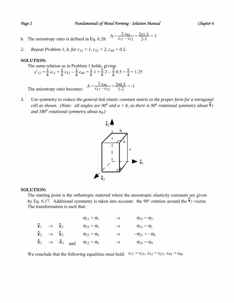
Page 2 Fundamentals of Metal Forming - Solution Manual Chapter 6
b. The anisotropy ratio is defined in Eq. 6.28: A = 2 c44
c11 - c12 = 2x1.5
2-1 = 3
2. Repeat Problem 1, b, for c11 = 1, c12 = 2, c44 = 0.5. SOLUTION: The same relation as in Problem 1 holds, giving:
c′12 = 3
8 c11 + 5
8 c12 - 3
4 c44 = 3
8 1 + 5
8 2 - 3
4 0.5 = 5
4 = 1.25
The anisotropy ratio becomes: A = 2 c44
c11 - c12 = 2x0.5
1-2 = -1
3. Use symmetry to reduce the general 6x6 elastic constant matrix to the proper form for a tetragonal cell as shown. (Note: all angles are 90o and a = b, so there is 90o rotational symmetry about x2 and 180o rotational symmetry about x3.)
c
b
a
x1
x2
x3 SOLUTION:
The starting point is the orthotropic material where the anisotropic elasticity constants are given by Eq. 6.17. Additional symmetry is taken into account: the 90° rotation around the x2 vector. The transformation is such that:
x1 → x3
x2 → x2
x3 → -x1 and
σ11 = σ1 → σ33 = σ3
σ33 = σ3 → σ11 = σ1
σ23 = σ4 → - σ21 = - σ6
σ12 = σ6 → σ23 = σ4
We conclude that the following equalities must hold: c 11 = c33, c12 = c23, c44 = c66

Chapter 6 Fundamentals of Metal Forming - Solution Manual Page 3
The anisotropic coefficients are then:
c11 c12 c13 0 0 0c12 c22 c12 0 0 0c13 c12 c11 0 0 00 0 0 c44 0 00 0 0 0 c55 00 0 0 0 0 c44
4. a. Is ψ (x, y) = x4 + y4 - 12x2y2 a valid Airy stress function in terms of both
equilibrium and compatibility requirements? Show why or why not. b. Assuming that the ψ (x, y) in Part a. is correct, find the stress components at the point
(1, 2). c. Find the strain components for the point (1, 2) assuming plane stress conditions (σ31 = 0).
Leave your answers in terms of general Young's modulus (E) and Poisson's ration (ν). SOLUTION: a. From:ψ = x4 + y4 - 6 x2 y2
we compute:
Ž4ψŽx4
= 24 ; Ž4ψŽy4
= 24 ; 2 Ž4ψ
Žx2 Žy2 = - 48
which shows that the compatibility condition (Eq. 6.59) is satisfied.
b. The stress components are computed according to:
σxx =
Ž2ψŽy2
= 12 y2 - 12 x2 ; σyy = Ž2ψŽx2
= 12 x2 - 12 y2 ; σxy = - Ž2ψ
Žx ∂y = 24 x y
The equilibrium equation is automatically satisfied; that can be verified on this peculiar case:
ŽσxxŽx
+ Žσxy
Žy = -24 x + 24 x = 0
ŽσxyŽx
+ Žσyy
Žy = 24 y - 24 y = 0
c. The corresponding strain components are as follows
εxx = 1 + νE
σxx - 1E
(σxx + σyy) = 12 1 + νE
(y2 - x2)
εyy = 1 + νE
σyy - 1E
(σxx + σyy) = 12 1 + νE
(x2 - y2)
εxy = 1 + νE
σxy = 24 1 + νE
xy
5. Given: ψ = 3xy5 + 3x5y - 10x3y3
a. Verify that ψ meets the condition for a proper Airy stress Function. Show your work.
Page 4 Fundamentals of Metal Forming - Solution Manual Chapter 6
b. Find the stresses as functions of x and y that correspond to ψ. c. Check to see if the stresses in Part b. satisfy equilibrium. Show your work. d. With a little manipulation using the stresses in Part b and Hooke's Law for plane stress,
obtain the strain functions shown below. Verify that these strain functions satisfy the compatibility conditions for strains. Show your work.
SOLUTION: a. The Airy function has the form: ψ = 3 x y55 + 3 x5 y - 10 x3 y3
We see that the partial derivatives in Eq. 6.59 are:
Ž4ψŽx4
= 360 x y ; Ž4ψŽy4
= 360 x y ; Ž4ψ
Žx2 ∂y2 = -360 x y
so that Eq. 6.59 which expresses the compatibility condition is satisfied.
b. We deduce the stress components according to:
σxx = Ž2ψŽy2
= 60 (x y3 - x3 y)
σyy = Ž2ψŽx2
= 60(x2 y - 12 x y3)
σxy = - Ž2ψ
Žx ∂y = -15 (x4 + y4) + 90 x2 y2
c. The equilibrium equation is automatically verified by stress components deduced from an Airy function, on our example we have:
ŽσxxŽx
+ Žσxy
Žy = 60 y3 - 180 x2 y + (- 60 y3 + 180 x2 y) = 0
ŽσxyŽx
+ Žσyy
Žy = - 60 y3 + 180 x2 y + 60 y3 - 180 x2 y = 0
εxx = 4 b (xy3 - x3y)
εyy = 4 b (x3y - xy3)
εxy = b (-x4 - y4 + 6x2y2)
where: b ≡ 15 (1 + ν)E
d. The components of the strain tensor are calculated in the following way:

Chapter 6 Fundamentals of Metal Forming - Solution Manual Page 5
εxx = 1 + νE
σxx - 1E
(σxx + σyy) = 60 1 + νE
(x y3 - x3 y)
εyy = 1 + νE
σyy - 1E
(σxx + σyy) = 60 1 + νE
(x3 y - x y3)
εxy = 1 + νE
σxy = 1 + νE
(- 15 x4 - 15 y4 + 90 x2 y2)
When we put b = 15 1 + ν
E , the desired form is obtained. The compatibility condition is written here:
Ž2εxx
Žy2 +
Ž2εyy
Žx2 - 2
Ž2εxy
Žx ∂y = 24 bxy + 24 bxy - 2 (24 bxy) = 0
6. Verify that Eqs. 6.38-6.42 follow from the traditional definitions of elastic constants.
SOLUTION: We consider a uniaxial tensile test in the x direction. Hooke's law in terms of Lamé coefficients (Eqs.6.31a-f) reduces to:
σxx = λ (εxx + 2 εyy) + 2 μ εxx
σyy = σzz = λ (εxx + 2 εyy) + 2 μ εyy = 0 These equations can be compared to Eq. 6.1 - 5 for the same case:
εxx = 1
E σxx ; εyy = - ν
E σxx or εyy = - ν εxx
We obtain the equalities:
σxx = E εxx = (λ(1 - 2 ν) + 2 μ) εxx
σyy = (λ(1 - 2 ν) - 2 μ ν) εxx = 0
From which we deduce by subtracting the second one to the first one: μ = E
2 (1 + ν)
Then μ is immediately deduced (provided 1 - 2 ): ν ≠ 0 λ = E ν2 (1 + ν) (1 - 2 ν)
From the Hooke's equation with the Lamé coefficients the equality G = μ is obvious. The bulk
modulus B is defined by: B =
13
σ11 + σ22 + σ33
ε11 + ε22 + ε33 = 1
K The easiest way to establish the relation is to consider a spherical strain tensor so that εxx = εyy = εzz = ε. According to Hooke's law, the stress state is σxx = σyy = σzz = (3 λ + 2 μ) ε,
and the bulk modulus is: B = λ + 2
3 μ

Page 6 Fundamentals of Metal Forming - Solution Manual Chapter 6
The other form of Hooke's equation is here: εxx = 1
E σxx - ν
E (σyy + σzz) = 1 - 2 ν
E σxx
so that the bulk modulus becomes:
B = σxx
3 1 - 2 νE
σxx = E
3 (1 - 2 ν)
Finally the relation between λ, μ and E, ν can be written: 2 (1 + ν) μ = E
(1 + ν) (1 - 2 ν) λ = E ν or
2 (1 + ν) μ = E
(1 - 2 ν) λμ
= ν
from which we deduce easily: ν = λ
2 (λ + μ) and E =
(3 λ + 2 μ) μ
λ + μ
7. Solve Eqs. 6.31 for strains and verify that the result is identical to Eqs. 6.1-5. SOLUTION:
First we see from Eqs. 6.31d-f and Eq. 6.38: for i ≠ j εij = 1
2μ σij = 1 + ν
E σij
Then we add Eqs. 6.31a-c: σkk�
k=1
3 = (3 λ + 2 μ) εkk�
k=1
3 or εkk�
k=1
3 = 1
3 λ + 2 μ σkk�k=1
3
Eq. 6.31a-c can be rewritten: εii = 2 μ σii - λ
2 μ (3 λ + 2 μ) σkk�k=1
3
Using Eqs. 6.38-39 and 6.42, we obtain:
λ2 μ (3 λ + 2 μ)
= νE
, so that the last equation is
transformed into: εii = 1 + ν
E σii - νE
σkk�k=1
3
, which is the desired result.
B. DEPTH PROBLEMS 8. Discuss any material restrictions which apply to the compatibility conditions Eqs. 6.52 and 6.55.
Consider anisotropy, elasticity vs. plasticity or other constitutive equations, possible presence of body forces, and the possibility of voids and cracks developing during deformation.
SOLUTION:
Eq. 6.52 does not use any additional physical assumption regarding the material. It is only based on the continuity of the third order derivatives of the displacement field. In the presence of cracks or a non differentiable boundary, this hypothesis must be analyzed carefully as the

Chapter 6 Fundamentals of Metal Forming - Solution Manual Page 7
displacement field may be discontinuous, thus violating the idea of a continuum of material upon which compatibility is based. On the other hand, Eq. 6.55 is established from Eq. 6.52 and the constitutive equation, so that it can be valid only for isotropic linear elasticity (with or without body forces). This equation must not be used for anisotropic elasticity, plasticity, elastoplasticity, etc.... An equivalent form can be derived for a given relationship between stress and strain for other cases.
9. a. Show that the elastic work done during small straining is given by
w = 1
2 cjkl εij εkl.
b. Write the elastic work in terms of stresses alone. c. Write results for parts a and b for the isotropic case.
SOLUTION: a. We suppose for convenience that the strain is applied with a so called radial loading, i. e. we
suppose that loading is performed from 0 to t, and that for any time τ, with 0 ≤ τ ≤ t, the strain
tensor is: ε ετ = τ
t ε ε
and the corresponding stress tensor: σ στ= c:ε ετ = τ
t c:ε ε
. During the time
increment dτ the strain increment is: dε ετ = dτ
t ε ε
, so that the increment of work is deduced with
the help of Eq. 4.54: dw = σ στ:dε ετ= τ
t c:ε ε :ε ε dτ
t
The total work is obtained by time integration: w = τ
t c:ε ε :ε ε dτ
t0
t = 1
2 c:ε ε :ε ε = 1
2 cijkl εij εkl�
ijkl The assumption of radial loading is not required since, by definition, the elastic response is conservative, i. e. no work is done in a closed loading cycle returning to the same loading state.
b. The compliance tensor s is introduced (see Exercise 6.1) which permits us to write: ε ε = s :σ σ and
the work in the form: w = 1
2 s :σ σ :σ σ = 1
2 sijkl σij σkl�
ijkl
c. The isotropic expressions are derived from Eqs. 6.31 and 6.1 - 4:
w = λ
2 εii�
i
2 + μ εij2�
ij = - ν
2 E σii�
i
2 + 1 + ν2 E
σij2�
ij
10. a. Show that Hooke's Law for an isotropic material may be written in the following form
εij = 2μ εij + ν
1 - 2ν εij δ ij

Page 8 Fundamentals of Metal Forming - Solution Manual Chapter 6
b. Find the equilibrium equation in indicial form in terms of strains alone. SOLUTION:
a. Hooke's law is written: σij = λ εkk δij + 2 μ εij = 2 μ (εij + λ
2 μ εkk δij )
with the help of Eq. 6.39 it is easy to obtain the desired result: σij = 2 μ (εij + ν
1 - 2ν εkk δij)
b. The equilibrium equation is expressed as: div(σ σ)i =
ŽσijŽxj
= 2 μ (ŽεijŽxj
+ ν1 - 2ν
ŽεkkŽxj
δij ) = 0
11. Consider a plane-strain isotropic linear elastic problem defined in a given domain. Assume the
displacement vector field takes the form:
u = μ1 = a x12 + 2b x1x2 + c x22
μ2 = a' x12 + 2b' x1x2 + c' x22
a. Write the strain tensor as a function of x1 and x2. b. Compute the stress tensor as a function of x1 and x2 with the isotropic Hooke law. c. Write the stress equilibrium equation assuming no body forces, and determine the relation
between the coefficients a, b, c, a', b', and c' that we must impose. d. Calculate the stress vector on each side of a square (see figure below).
-11
-1
1
x1
x2
0
Verify that the external forces on the square are in equilibrium when the condition defined in Part c is fulfilled.
SOLUTION: a. The derivatives of the displacement components are
Žu1Žx1
= 2 a x1 + 2 b x2, Žu1Žx2
= 2 b x1 + 2 c x2
Žu2Žx1
= 2 a′ x1 + 2 b′ x2, Žu2Žx2
= 2 b′ x1 + 2 c′ x2
Chapter 6 Fundamentals of Metal Forming - Solution Manual Page 9
The strain rate tensor is immediately obtained: ε =
2 a x1 + 2 b x2 (b+a′) x1 + (c+b′)x2
(b+a′) x1 + (c+b′)x2 2 b′ x1 + 2 c′ x2
b. The components of stress tensor are now:
σ11 = 2λ (a+b′) x1 + (b+c′) x2 + 4 μ (a x1 + b x2)
σ12 = 2 μ (b+a′) x1 + (c+b′)x2
σ22 = 2λ (a+b′) x1 + (b+c′) x2 + 4 μ ( b′ x1 + c′ x2)
c. The equilibrium equation is written:
Žσ11Žx1
+ Žσ12Žx2
= 2 λ (a+b′) + 4 μ a + 2 μ (c+b′) = 0
Žσ12Žx1
+ Žσ22Žx2
= 2 μ (b+a′) + 2 λ (b+c′) + 4 μ c′ = 0
d. The stress vector on the upper side and its integral on this side are:
σ12σ22
= 2 μ (b+a′) x1 + (c+b′)
2λ (a+b′) x1 + (b+c′) + 4 μ ( b′ x1 + c′) ,
σ12σ22
dx1-1
1 =
4 μ (c+b′)
4 λ (b+c′) + 8 μ c′ On the lower side:
- σ12- σ22
= - 2 μ (b+a′) x1 - (c+b′)
-2λ (a+b′) x1 - (b+c′) - 4 μ ( b′ x1 - c′) ,
-σ12-σ22
dx1-1
1 =
4 μ (c+b′)
4 λ (b+c′) + 8 μ c′ On the right hand side:
σ11σ12
= 2λ (a+b′) + (b+c′) x2 + 4 μ (a + b x2)
2 μ (b+a′) + (c+b′)x2 ,
σ11σ12
dx2-1
1 =
4λ (a+b′) + 8 μ a
4 μ(b+a′) On the left hand side:
-σ11-σ12
= - 2λ -(a+b′) + (b+c′) x2 - 4 μ (a + b x2)
-2 μ (b+a′) - (c+b′)x2 ,
-σ11-σ12
dx2-1
1 =
4λ (a+b′) + 8 μ a
4 μ(b+a′) When all these contribution are added and the result equated to zero we obtain:
, which are equivalent to the equations we found in c.
4 μ (c+b′) + 4 λ (a+b′) + 8 μ a = 0
4 λ (b+c′) + 8 μ c′ + 4 μ (b+a′) + 0
12. Consider 3 elastic bars of equal length which are pinned at the ends as shown and to which a vertical force F is applied.
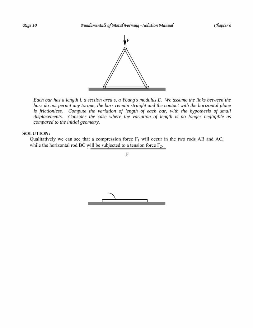
Page 10 Fundamentals of Metal Forming - Solution Manual Chapter 6
F
Each bar has a length l, a section area s, a Young's modulus E. We assume the links between the bars do not permit any torque, the bars remain straight and the contact with the horizontal plane is frictionless. Compute the variation of length of each bar, with the hypothesis of small displacements. Consider the case where the variation of length is no longer negligible as compared to the initial geometry.
SOLUTION:
Qualitatively we can see that a compression force F1 will occur in the two rods AB and AC, while the horizontal rod BC will be subjected to a tension force F2.
FA
B CF2
F1 F1
α
The equilibrium of vertical forces at point A gives: F = 2 F1 sin(60°) or F1 = F/ 3. If the length variation Δl1 of AB or AC is introduced, we have also:
F1 = F/ 3 = E a Δl1
l or Δl1 = F l
E a 3
The horizontal force exerted in B on rod BC by rod AB is: F2 = F1 cos(60°) = F
2 3 and the
length variation Δl2 of BC is computed by: F2 = F
2 3 = E a Δl2
l or Δl2 = F l
2 3 E a
When the displacements are no longer neglected, we suppose that the new lengths of the rods are: AB = AC → l1 = l + Δl1; BC → l2 = l + Δl2
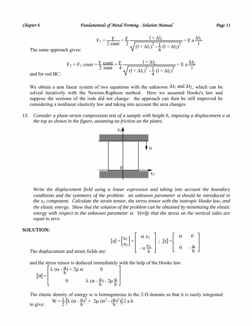
Chapter 6 Fundamentals of Metal Forming - Solution Manual Page 11
The same approach gives:
F1 = F2 sinα
= F2
l + Δl1(l + Δl1)2 - 1
4 (l + Δl2)2
= E a Δl1l
and for rod BC:
F2 = F1 cosα = F2
cosαsinα
= F4
l + Δl2(l + Δl1)2 - 1
4 (l + Δl2)2
= E a Δl2l
We obtain a non linear system of two equations with the unknown Δ , which can be solved iteratively with the Newton-Raphson method. Here we assumed Hooke's law and suppose the sections of the rods did not change: the approach can then be still improved be considering a nonlinear elasticity law and taking into account the area changes.
l1 and Δl2
13. Consider a plane-strain compression test of a sample with height h, imposing a displacement u at
the top as shown in the figure, assuming no friction on the plates.
0
u
x2
x1
Write the displacement field using a linear expression and taking into account the boundary
conditions and the symmetry of the problem: an unknown parameter α should be introduced in the x1 component. Calculate the strain tensor, the stress tensor with the isotropic Hooke law, and the elastic energy. Show that the solution of the problem can be obtained by minimizing the elastic energy with respect to the unknown parameter α. Verify that the stress on the vertical sides are equal to zero.
SOLUTION:
The displacement and strain fields are:
u = u1u2
= α x1
- u x2h
; ε = α 0
0 - uh
and the stress tensor is deduced immediately with the help of the Hooke law:
σ = λ (α - u
h) + 2μ α 0
0 λ (α - uh
) - 2μ uh
The elastic density of energy w is homogeneous in the 2-D domain so that it is easily integrated
to give: W = 1
2 λ (α - u
h)2 + 2μ (α2 - (u
h)2) 2 a h
Page 12 Fundamentals of Metal Forming - Solution Manual Chapter 6
where 2 a is the width of the sample. Minimization of the elastic energy yields:
ŽWŽα
= 0 = λ (α - uh
) + 2μ α 2 a h
The optimum parameter is: α = λ
λ + 2 μ uh
and the corresponding stress tensor is written:
σ = 0 0
0 - 4μ λ+μ
λ+2μ λ u
h
We see that it is the exact solution of our problem.
14. Repeat Problem 13 for a cubic crystal where x1 and x2 are oriented along four-fold symmetry axes.
SOLUTION: The displacement and strain fields are the same as those in problem 13, the non zero components
of the stress tensor become:
σ11 = c11 ε11 + c12 ε22σ22 = c12 ε11 + c11 ε22
The elastic energy is derived according to:
W = 12
(c11 ε112 + 2 c12 ε22 ε11 + c11 ε22
2 ) 2 a h
The minimization of the elastic energy is achieved by putting:
ŽWŽα
= (c11 α +c12 (- uh
)) 2 a h ⇒ α = c12c11
uh
The final solution in stress is:
σ11 = 0 , σ22 = - c112 - c12
2
c11 uh
15. Repeat Problem 13 with a 3-D sample and an orthotropic material. SOLUTION:
The approach is similar to that of problems 13 and 14. We have:
Chapter 6 Fundamentals of Metal Forming - Solution Manual Page 13
u1u2u3
=
α x1
β x2
- uh
x3
ε =
α 0 0
0 β 0
0 0 - uh
The non-zero components of the stress tensor are calculated with Eq. 6.17:
σ11 = c11 α + c12 β + c13 (- uh
)
σ22 = c12 α + c22 β + c23 (- uh
)
σ33 = c13 α + c23 β + c33 (- uh
)
and the elastic energy takes the form:
W = 1
2 4abh c11 α2 + c22 β2 + c33 (- u
h)2 + 2 c12 α β + 2 c13 α (- u
h) + 2 c23 β (- u
h)
if 2a is the length and 2b the width of the sample. Minimization with respect to the two unknown parameters gives the linear system of two equations:
ŽWŽα
= 0 = 4abh c11 α + c12 β + c13(- uh
) ⇒ σ11 = 0
ŽWŽβ
= 0 = 4abh c12 α + c22 β + c33(- uh
) ⇒ σ22 = 0
The solution of which is:
α = c22 c13 - c12 c23
c11 c22 - c122
uh
β = c11 c23 - c12 c13
c11 c22 - c122
uh
16. Show that the only incompressible isotropic elastic medium is a liquid by computing the shear modulus, μ.
SOLUTION:
An isotropic linear elastic medium which obeys Hooke's law is incompressible if (see
Eq. 6.1 - 5): 0 = ε11 + ε22 + ε33 = 1 - 2 ν
E (σ11 + σ22 + σ33)
, which holds when ν = 0.5.
According to Eq. 6.41 we can also write:
12
= λ2 (λ+ μ) , that is μ = 0 for any finite value of λ, so
that σij = 0 for any i ≠ j. Moreover the diagonal terms of the stress tensor do not depend on the strain tensor so that by isotropy we have: σ . That corresponds to an inviscid fluid.
11 = σ22 = σ33 = - p
17. The Airy Stress Function for a screw dislocation in an isotropic crystal is given by

Page 14 Fundamentals of Metal Forming - Solution Manual Chapter 6
ψ = μby
4π (1-ν) ln x2 + y2 ,where b = Burger's vector, a small constant.
a. Find the stresses and strains for the screw dislocation.
b. Is compatibility satisfied everywhere? Why or why not? c. Do plane strain or plane stress condition hold?
SOLUTION:
a. We first put k =
μ b4 π (1 - ν) and r in order to simplify the expressions. Eq. 6.46 gives
the stress components:
2 = x2 + y2
σxx =
Ž2ψŽy2 = 2 k y
3 x2 + y2
r4 , σyy =Ž2ψŽx2 = 2 k y
y2 - x2
r4 , σ xy = -Ž2ψŽx ∂y
= 2 k xy2 - x2
r4
According to Eq. 6.1 - 5 the strain components are:
εxx = 2 k y
r41E
(3 x2 + y2) -νE
(y2 - x2) , εyy = 2 k yr4
- νE
(3 x2 + y2) + 1E
(y2 - x2)
εzz =- νE 4 k
yr2 , εxy =
1 + νE 2 k x
y2 - x2
r4
b. We put: ϕ =
Ž2ψŽx2
+ Ž2ψŽy2
= 4 k yr2
we have to compute:
Ž2ϕŽx2
= - 8 k y (y2 - 3 x2)r2
and Ž2ϕŽy2
= 8 k y (y2 - 3 x2)r2
so that the compatibility condition:
Ž2ϕŽx2
+ Ž2ϕŽy2
= 0 is fulfilled everywhere except at the origin.
c. The mechanical problem is obviously plane stress but not plane strain.
18. The elastic fields of a screw dislocation are most simply derived by considering the displacements in polar coordinates:
uz (r, θ) = bθ
2π = b
2π tan-1 yx, where b = the Burger's vector, a small constant.
a. Find the stresses and strains for the screw dislocation. b. Is compatibility satisfied everywhere? Why or why not?

Chapter 6 Fundamentals of Metal Forming - Solution Manual Page 15
c. Do plane strain or plane stress conditions hold?
SOLUTION: a. From the given displacement field we compute the strain and stress tensors in the usual way:
ux = 0
uy = 0
uz = b2π
tan-1yx
→ ε =
0 0 - b′2
yr2
0 0b′2
xr2
- b′2
yr2
b′2
xr2
0
→ σ =
0 0 - μb′ yr2
0 0 μb′ xr2
- μb′ yr2
μb′ xr2
0
where we put: r2 = x2 + y2 and b′ = b
2π
b. Compatibility is necessarily satisfied everywhere (except at the origin) as the strain tensor is obtained by differentiation of a displacement field.
c. By examining the strain and stress tensors we conclude that we have both plane strain and stress tensor fields (with respect to plane Oxy).

CHAPTER 7 - PROBLEM SOLUTIONS
A. PROFICIENCY PROBLEMS 1. What is the meaning of stress states lying outside of yield surface? SOLUTION:
They are states accessible only by changing the material properties - by strain hardening or heat treatment perhaps. In either case, the yield surface must change in order to achieve these stresses.
2. A researcher has found a way to measure the yield surface of sheet metal rapidly and automatically. He inserts a sheet into a biaxial testing machine and loads along proportional paths until, while he measures strains in the two directions, he obtains the 0.2% offset strength. Then he unloads, chooses a slightly different ratio and does the same thing, until he has generated many yield points.
Criticize this procedure. SOLUTION:
The major criticism is that the material properties are different after the first and each subsequent test because the approximately 0.002 plastic strains accumulate and the material strain hardens. Therefore, the various yield stresses measured are not for a single material and do not represent a yield surface at an instant. A secondary criticism is the use of the 0.002 offset strength as the yield strength. In practice, this is not a very practical problem, but the yield strength measured in this way could be considerably greater or less than the actual yield.
3. Critically evaluate the yield functions presented below in terms of isotropy, pressure-dependence,
and existence of a Bauschinger effect. Demonstrate your results. Why would you choose to use each yield function?
a. Hill's1 Quadratic Yield Function (1948)
f = F σ2 - σ3
2 + G σ1 - σ32 + H σ1 - σ2
2
b. Hill's2 Non-Quadratic Yield Function (1979)
f = F σ2-σ3
M + G σ1-σ3M + H σ1-σ2
M
c. Bourne and Hill3 (σ3 = 0, not principal axes):
f = 3σx
3 - 6σ x2σy - 6σxσy
2 + 4σy3 + (4σx+21σy) σ xy
2
1 R. Hill: The Mathematical Theory of Plasticity, Clarendon Press, 1950, p. 318. R. Hill: Proc. Roy. Soc., 1949, vol. 198, p. 428. 2 R. Hill: Math. Proc. Camb. Philos. Soc., 1979, vol. 85, p. 179. P.B. Mellor and A. Parmar, Mechanics of Sheet Metal Forming, D.P. Koistinen and N.M. Wang, Plenum Press, 1978, p.67. 3 L. Bourne and R. Hill: Philos. Mag., 1950, vol. 41, p. 671.

Page 2 Fundamentals of Metal Forming - Solution Manual Chapter 7
d. Drucker4: f = J 2
′ 3– c J3
′ 2, where c = constant
e. Edelman and Drucker5:
f = 1
2 cijkl σ ij′ - M εij
P σkl′ - M εkl
P , cijkl, M = constants, εkl = plastic strain
f. Gotoh6 (σ3 = 0):
f = A o σx+σy4+A 1σx
4+A 2σx3σy+A3σ x
2σy2+A 4σxσy
3+A 5σy4
+ A6σx2+A 7σxσ y+A8σy
2 σxy2+A 9σxy
4, A 1 = constants.
g. Bassani7 (σ3 = 0):
f = σ1 + σ 2
N + (1 + 2r) k σ1 - σ2M,
r, k, M = constants. h. Jones & Gillis8 (σ3 = 0):
f = c11σx
2 + c 12σxσy + c13σxσxy + c22σy2 + c 23σyσxy + c33τxy
2, cij = constants
i. Gupta9: f = J 2
′ - αp J1, α = constant.
SOLUTION: a. • Not isotropic (unless F = G = H)
• Pressure-independent [since f σ i + p = f σ i ]
• No Bauschinger effect [since f σ i = f –σ i ] • Modification of von Mises to handle simple anisotropy - for example, for rolled sheet.
Allows different strains in two lateral directions in tensile test. b. • Not isotropic (unless F = G = H) • Pressure-independent • No Bauschinger effect • Includes the anisotropy of Part a., but allows further adjustment of shape to account for
higher or lower flow strength in plane-strain or balanced biaxial tension (relative to uniaxial tension) for a given r value.
c. • Not isotropic • Cannot determine pressure-dependence since only two principal stresses are represented • A Bauschinger effect is inherent (because of the cubic terms) • This is a purely 2-D yield function with fixed constants that was fit to experimental data from
4 D.C. Drucker: J. Appl. Mech., Trans. ASME, 1949, vol. 16, p. 349. 5 F. Edelman and D.C. Drucker: J. Franklin Inst., 1951, vol. 251, p. 581. 6 M. Gotoh: Int. J. Mech. Sci., 1977, vol. 19, p.505. 7 J.L. Bassani: Int. J. Mech. Sci., 1977, vol. 19, p. 651. 8 (unpublished) 9 Y.M. Gupta: Acta Metall., 1977, vol. 25, p. 1509.

Chapter 7 Fundamentals of Metal Forming - Solution Manual Page 3
tensile tests conducted at various angles in a sheet of metal. It provides a detailed variation of σy vs. θ but has no consistent 3-D form.
d. • Isotropic (use of invariants proves this) • Pressure-independent (use of deviatoric components demonstrates this) • No Bauschinger effect (the odd invariant, , has been squared to avoid this. J3
′
• This is a very interesting generalization of the simplest yield function, , which satisfies pressure-independence, isotropy, and no Bauschinger effect. Because it is isotropic, it cannot contribute to fitting strain ratio effects on sheet tensile tests, however. It is similar in concept to Part b., with F = G = H.
J2′ = k
e. • Not isotropic (unless ) Cijkl = Cmnop, M = 0, or ε ij = 0 • Pressure-independent (from use of deviatoric components) • Bauschinger effect (unless M = 0) • This is the logical extension to the most general quadratic yield function in terms of
anisotropy, with kinematic hardening depending on total plastic strain. f. • Not isotropic • Cannot determine pressure-dependence since only two principal stresses are represented • A Bauschinger effect is inherent (because of the cubic power terms) • This is a purely 2-D yield function with fixed constants that was fit to experimental data from
tensile tests conducted at various angles in a sheet of metal. It provides a detailed variation of σy vs. θ but has not consistent 3-D form.
g. • Isotropic (cannot distinguish σ1 and σ2 because of absolute values) • Cannot determine pressure dependence since only two principal stresses are represented • A Bauschinger effect is present (unless N and M are even) • Very similar to Part b., but the different power for the two terms means it must be handled
numerically. h. • See Parts c. and f. i. • Isotropic (use of invariants) • Pressure-dependent (unless ) αp = 0
• Bauschinger effect (unless ) αp = 0 • This yield function is the simplest one which includes a pressure dependence, which is its
purpose. For example, compressible materials such as powders or sponges could be treated with this function.
4. Write each of the yield functions in Problem 3 in terms of each of the following definitions of
effective stress:
a. tensile test in the x1 direction, σ = σ1 b. tensile test in the x2 direction, σ = σ2

Page 4 Fundamentals of Metal Forming - Solution Manual Chapter 7
c. balanced biaxial test, σ1 = σ 2 = σ d. shear test, same principal axes, σ1 = σ , σ2 = – σ
SOLUTION:
a. x1 tension: G + H σ2 = f
x2 tension: F + H σ2 = f
Bal. Biax: F + G σ2 = f
Shear (assume that occurs from principal axes, i.e. as stress state consisting of is equivalent to
τ = τxy′ 45° τxy
σ1 = σ, σ2 = –σ:
F + G + 4H σ 2 = f
b. x1 tension: = G + H σM = f
x2 tension: F + H σM = f
Bal. Biax: F + G σ M = f
Shear: F + G + 2MH σM (where σ1 = σ, σ2 = –σ)
c. x1 tension: 3 σ3 = f x2 tension: 4 σ3 = f Bal. Biax: –5 σ3 = f Shear: –σ3 = f (where σ1 = σ, σ2 = –σ)
d.
x1 tension: σ =σ 0 00 0 00 0 0
, σ′ =
23σ 0 00 – 1
3σ 00 0 – 1
3 σ
Chapter 7 Fundamentals of Metal Forming - Solution Manual Page 5
J2
′ = – σ11′ σ22
′ + σ22′ σ33
′ + σ11′ σ33
′ = – 23 – 1
3 σ2 + – 13 – 1
3 σ2 + 23 – 1
3 σ 2 = 13 σ2
J3′ = σ11
′ σ22′ σ33
′ = 227 σ3
1
27 σ6 – C 4729 σ6 = 1
27 1 – 427 C σ6 = f
Same as x because of isotropy x2 tension: 1
Bal. Biax: σ =σ 0 00 σ 00 0 0
, σ′ =
13σ 0 00 1
3σ 00 0 –2
3σ
This is the same as x and tension because of a) isotropy and b) no Baushinger effect, so that a stress state of σ
1 x2
ij is equivalent to - σij
Shear: σ =
σ 0 00 – σ 00 0 0
, σ′ =σ 0 00 – σ 00 0 0
J2′ = – –σ2 + 0 + 0 = σ2
J3
′ = σ11′ σ22
′ σ33′ = 0 , so σ6 = f [same as von Mises]
e.
x1 tension: σ′ =
23σ 0 00 – 1
3σ 00 0 – 1
3σ
For simplicity, we assume no initial loading, such that εij = 0, then:
12 C1111
23
23 σ2 + C1122
23 –1
3 σ2 + C113323 –1
3 σ2 +
C2211 –13
23 σ 2 + C2222 –1
3 –13 σ2 + C2233 –1
3 –13 σ2 +
C3311 – 13
23 σ2 + C3322 – 1
3 –13 σ 2 + C3333 –1
3 –13 σ2 = f

Page 6 Fundamentals of Metal Forming - Solution Manual Chapter 7
σ2
18 4 C1111 –2 C1122 + C1133 + C2211 + C3311 + C2222 + C2233 + C3322 + C3333 = f
x2tension:
σ2
18 4 C2222 –2 C1122 + C2211 + C3311 + C1133 + C1111 + C3333 + C1133 + C3311 = f
Bal. Biax: σ 2
18 4 C3333 –2 C1133 + C3311 + C2233 + C3322 + C1111 + C2222 + C1122 + C2211 = f
Shear: σ 2
2 C1111 + C2222 – C1122 – C2211 = f, where: σ1 = σ, σ2 = – σ
f. x1 tension: σ4 A 0 + A 1 = f
x2 tension: σ4 A 0 + A 5 = f
Bal. Biax: σ4 16 A 0 + A 1 + A 2 + A 3 + A 4 + A 5 = f
Shear: σ4 A 1 – A 2 + A 3 – A 4 + A 5 = f , where: σ 1 = σ, σ2 = –σ
g. x1 tension: σN + 1 + 2r K σM = f
x2 tension: σN + 1 + 2r K σM = f
Bal. Biax: 2N σN = f
Shear: 1 + 2r k 2M σM = f , where: σ1 = σ, σ 2 = –σ
h. x1 tension: c11 σ 2 = f
x2 tension: c22 σ 2 = f Bal. Biax: c11 σ2 + c12 σ2 + c22 σ2 = f Shear: c11 σ2 – c12 σ 2 + c22 σ2 = f, where: σ1 = σ, σ 2 = –σ

Chapter 7 Fundamentals of Metal Forming - Solution Manual Page 7
i. x1 tension: J2
′ = 13 σ 2 J1 = σ , therefore: 1
3 σ – αp σ = 13 – α p σ = f
x2 tension: (same as x1, isotropic)
Bal. Biax: J2
′ = 13 σ2 , J1 = 2 σ, therefore: 1
3 – 2 αp σ = f
Shear: J 2
′ = σ2 J1 = 0 , therefore: σ = f, where: σ1 = σ, σ 2 = – σ
5. Derive the normality condition for each of the yield functions in Problem 3. SOLUTION:
a. dε1 = 2dλ G + H σ1 – Hσ2 – G σ3
dε2 = 2dλ F + H σ2 – Hσ1 – F σ3
dε3 = 2dλ F + G σ3 – Gσ1 – F σ2
b. Assume that (other cases can be handled separately), then: σ1 > σ2 > σ3 > 0
dε1 = Mdλ G σ1 – σ 3
M–1+ H σ1 – σ2
M–1
dε2 = Mdλ F σ2 – σ3
M–1– H σ1 – σ2
M–1
dε3 = Mdλ –F σ2 – σ3
M–1– G σ1 – σ3
M–1
c. dεx = dλ 9 σx
2 – 12 σx σy – 6 σy2 + 4 σxy
2
dεy = dλ –6 σ x
2 – 12 σx σy + 12 σy2 + 21 σxy
2
dεxy = dλ 4 σx + 21 σy 2σ xy
d.
dε1 = dλ ∂f
∂σ1= dλ 3 J2
′ 2 ∂J 2′
∂σ1– 2 c J3
′ ∂J 3′
∂σ1= dλ 3 J2
′ 2σ1
′ – 23 c J 3
′ J2′ + 3σ2
′σ3′
Page 8 Fundamentals of Metal Forming - Solution Manual Chapter 7
= dλ J 2′ 2
2σ 1 – σ2 – σ3 – 29 c J3
′ 2σ12 – σ2
2 – σ32 – 2σ1 σ2 – 2σ1 σ3 + 4σ2 σ3
dε2 = dλ ∂f
∂σ2= dλ 3 J2
′ 2 ∂J 2′
∂σ2– 2 c J3
′ ∂J 3′
∂σ2= dλ 3 J2
′ 2σ2
′ – 23 c J 3
′ J2′ + 3σ1
′σ3′
= dλ J 2′ 2
2σ 2 – σ1 – σ3 – 29 c J3
′ 2σ22 – σ1
2 – σ32 – 2σ1 σ2 + 4σ 1 σ3 – 2σ2 σ3
dε3 = dλ ∂f
∂σ3= dλ 3 J2
′ 2 ∂J 2′
∂σ3– 2 c J3
′ ∂J 3′
∂σ3= dλ 3 J2
′ 2σ3
′ – 23 c J 3
′ J2′ + 3σ1
′σ2′
= dλ J 2′ 2
2σ 3 – σ1 – σ2 – 29 c J3
′ 2σ32 – σ1
2 – σ22 + 4σ1 σ2 – 2σ 1 σ3 – 2σ2 σ3
where, from Eqs. 3.34 and 3.35:
J2
′ = 16 σ1 – σ2
2 + σ1 – σ32 + σ 2 – σ3
2 = 13 σ 1
2 + σ22 + σ3
2 – 13 σ1σ2 + σ1σ3 + σ2σ3
J 3′ = σ1
′ σ2′ σ3
′ = 127 2σ1 – σ 2 – σ3 2σ2 – σ1 – σ3 2σ 3 – σ1 – σ2
= 227 σ1
3 + σ 23 + σ3
3 – 19 σ1σ 2
2 + σ12σ2 + σ1σ3
2 + σ12σ3 + σ2σ3
2 + σ22σ 3 + 4
9 σ1 σ2 σ3
e. Consider only the start of deformation, when and write in principal axes. ε ijP = 0,
, f = Cij σ i′ σ j
′
∂f
∂σm= Cij
∂∂σm
σ i′ σ j
′ = Cij σ i′∂σ j
′
∂σm+ σ j
′ ∂σ1′
∂σm
but note that since , where , that σ i′ = 2 σ i – σ j – σ k i ≠ j ≠ k
∂σ j′
∂σm= 2 if j = m
– 1 if j ≠ m
Therefore, we can write:
dε1
dλ = 2 2C11 + C12 + C13 + C21 + C31 σ1′
– 1 2C22 + C21 + C23 + C12 + C13 σ2′
– 1 2C33 + C31 + C32 + C13 + C23 σ3′
, or
Chapter 7 Fundamentals of Metal Forming - Solution Manual Page 9
dε1
dλ = 23 2C11 + C12 + C13 + C21 + C31 2σ 1 – σ2 – σ3
– 13 2C22 + C21 + C23 + C12 + C13 2σ2 – σ 1 – σ3
– 13 2C33 + C31 + C32 + C13 + C23 2σ3 – σ 1 – σ2
The other components follow by inspection. (For example would look the same except that
the coefficients on the three terms would be, respectively,
dε2
– 13, 2
3 , – 13 , or for the
coefficients would become
dε2
– 13, – 1
3 , 23 .
f. dεx
dλ= 4A o σx + σ y
3 + 4A 1σx3 + 3A 2σx
2σy + 2A 3σxσy2 + A 4σy
3 + 2A 6 σxσxy2 + A 7σyσ xy
2
dεy
dλ= 4A o σx + σ y
3 + A 2σx3 + 2A 3σx
2σ y + 3A 4σxσy2 + 4A 5σy
3 + A 7σxσxy2 + 2A 8σyσxy
2
dεxy
dλ= 2 A 6σx
2 + A 7σxσy + A 8σy2 σxy + 4A 9σxy
3
g. Assume that for simplicity. Other cases may be derived separately. σ1 > σ2 > 0
dε1 = dλ N σ 1 + σ2
N–1 + 1 + 2r k M σ1 – σ2M–1
dε2 = dλ N σ 1 + σ2
N–1 – 1 + 2r M σ1 – σ2M–1
h. dεx = dλ 2c11 σx + c12 σy + c13σxy
dεy = dλ c12 σx + 2c22 σy + c23σxy
dεxy = dλ c13 σx + 2c23 σy + 2c33σxy
i.
J2
′ = +16 σ1
2 – σ22 2
+ σ12 – σ 3
2 2+ σ2
2 – σ32 2
, J1 = σ1 + σ2 + σ3
f = J2
′12 – α p J1 , therefore:
∂f∂σ1
= 12 J2
′ – 12 ∂ J2
′
∂ σ 1– α p
∂ J1
∂ σ 1

Page 10 Fundamentals of Metal Forming - Solution Manual Chapter 7
dε1dλ =
2 σ1 – σ2 – σ3
6 J 2′
– αp =2 σ1 – σ2 – σ3
σ1 – σ22 + σ2 – σ3
2 + σ1 – σ32
12
– αp
dε2, dε3 follow directly
6. Assume that σi3 = 0 and that we are working in principal axes for each yield function in Problem
3. Letting α = σ2/σ1 and β , find expressions for α(β) and for β(α). = dε2/dε1
SOLUTION:
a.
β = dε2
dε1=
F + H σ2 – H σ1
G + H σ1 – H σ2
=F + H α – H
G + H – H α
α = σ 2
σ 1=
β G + H + HF + H + β H
b. Assuming that : σ1 > σ2 > 0
β =
dε2
dε1=
F σ2M–1 – H σ1 – σ2
M–1
G σ1M–1 + H σ1 – σ2
M–1 =F αM–1 – H 1 – α M–1
G αM–1 + H 1 – α M–1
(Because of the form, α = ? α β is transcendental, so α β must be found numerically.)
c.
β =
dεy
dεx=
–6 – 12 α + 12 α2
9 – 12 α – 6 α2
α =
– 2 β – 1 ± 10 β2 + 8 β + 12
2 β + 2 ,
which is found by using the quadratic formula on β α .
d.
dε1 = dλ 1
3 σ12 + σ2
2 – σ1 σ2 2 σ1 – σ2 – 2243 2 σ 1 – σ2
, or
= dλ 2 σ2 – σ1 σ1 + σ2 2 σ1
2 – σ22 – 2 σ1 σ2
dε2 = dλ 1
3 σ12 + σ2
2 – σ1 σ2 2 σ2 – σ1 – 2243 2 σ 1 – σ2
, or

Chapter 7 Fundamentals of Metal Forming - Solution Manual Page 11
= dλ 2 σ2 – σ1 σ1 + σ2 2 σ2
2 – σ 12 – 2 σ1 σ2
β = dε2dε1
=
2α – 1 1 + α2 – α – 281 2 – α 1 + α 2 α2 – 1 – 2α
2 – α 1 + α 2 – α – 281 2α – 1 1 + α 2 – α2 – 2α
hopeless to do in closed form unless the numerator and denomerator can be factored. α =
e.
β = dε2
dε1=
c12 + c21 2σ1 – σ2 +c22 2σ2 – σ1 + c23 + c32 – σ1 – σ2
2 c11 2σ1 – σ2 + c12 + c21 2σ2 – σ1 + c13 + c31 – σ1 – σ2
β =
c12 + c21 2 – α +c22 2α – 1 + c23 + c32 – 1 – α
2 c11 2 – α + c12 + c21 2α – 1 + c13 + c31 – 1 – α
α =
2 c12 + c21 – c22 – c23 – c32 + β – 4 c11 +c12 +c21 +c13 +c31
c12 + c21 + c23 + c32 – 2 c22 + β – 2 c11 +2 c12 +c21 – c13 –c31
f.
β = dε2
dε1=
4 A 0 1 + α 3 + A 2 + 2 A 3 α + 3 A 4 α2 + 4 A 5 α3
4 A 0 1 + α 3 + 4 A 1 + 3 A2 α + 2 A 3 α2 + A 4 α 3
is a cubic equation and may be solved numerically or in closed form. α(β)
g.
β = dε2
dε1=
N 1 + α N–1 – 1 + 2r M 1 – α M–1
N 1 + α N–1 + 1 + 2r M 1 – α M–1
α(β) = transcendental
h. β = dε2
dε1= c12 + 2 c22 α
2 c11 + c12 α
α = c12 – 2 β c11
β c12 – 2 c22
Page 12 Fundamentals of Metal Forming - Solution Manual Chapter 7
i.
dε1 = 2 σ1 – σ2
2 σ12 + σ 2
2 – σ1 σ2
– αp , and dε2 = 2 σ2 – σ 1
2 σ12 + σ2
2 – σ1 σ2
– αp
β = dε2
dε1=
2 α – 1 – α p 2 σ12 + σ2
2 – σ1 σ 2
2 – α – αp 2 σ12 + σ2
2 – σ1 σ2 appears to be transcendental, and thus must be found numerically. α(β)
7. Construct a full set of useful equations expressed in principal axes for the following yield functions. Useful equations include the yield function in terms of σ, the associated flow rule, the normality equations (forward and inverse), definition of dλ in terms of σ and dε (where x1 tension is the standard state), dε in terms of dε1, dε2 and dε3, α(β), and β(α); where α = σ2/σ1 and
. (The last sets of equations were derived in Problem 6.) β = dε2/dε1
a. von Mises: f = (σ1-σ2)2 + (σ1-σ 3)
2 + (σ 2-σ3)2
b. Hill quadratic: f = F(σ 2-σ3)
2 + G(σ1-σ3)2 + H(σ1-σ 2)
2
c. Hill normal anisotropic: modify function #2 such that the x1 and x2 axes are equivalent
and the strain ratio dε2/dε1 in an x1 tensile test is r. (x3 is the sheet-thickness direction).
d. Hill non-quadratic (Case IV), (σ3 = 0):: f = (1+2r) |σ1-σ2|
M + |σ1+σ2|M
(You may restrict your attention to one octant, where σ2>σ1>0).
e. Bassani 2-D (σ3 = 0): f = σ 1+σ2
N + (1+2r) k σ 1-σ2M
SOLUTION:
a. von Mises: f = σ1 – σ 2
2 + σ1 – σ32 + σ2 – σ3
2
x1 - Yield:
σ = 1
2σ1 – σ2
2 + σ1 – σ32 + σ2 – σ 3
212
Flow Rule:
dε12 σ1 – σ2 – σ3
= dε22 σ2 – σ1 – σ3
= dε32 σ3 – σ1 – σ2
= dε i
σ i′
Normality: dε1 = 2dλ 2 σ1 – σ2 – σ3
dε2 = 2dλ 2 σ2 – σ1 – σ3

Chapter 7 Fundamentals of Metal Forming - Solution Manual Page 13
dε3 = 2dλ 2 σ3 – σ1 – σ2
Normality (inverse): σ1 – σ2 = 1
6dλ dε1 – dε2
σ2 – σ3 = 1
6dλ dε2 – dε3
σ1 – σ3 = 1
6dλ dε1 – dε3
Lambda: dλ = dε
4σ based on usage shown above
Effective Strain:
dε = 2
3 dε1 – dε22
+ dε2 – dε32+ dε1 – dε3
212
= 2
3 dε12 + dε2
2 + dε32
12
Ratios σ3 = 0 :
α = σ2σ1
= 2β + 12 + β
β = dε2dε1
= 2α – 12 – α
b. Hill quadratic: f = F σ 2 – σ3
2 + G σ1 – σ32 + H σ1 – σ 2
2
x1 - Yield:
σ =
1G + H
F σ2 – σ32 + G σ1 – σ3
2 + H σ1 – σ22
12
Flow Rule:
dε1
G σ1 – σ3 + H σ1 – σ2=
dε2
F σ2 – σ3 – H σ1 – σ2=
dε3
–F σ2 – σ3 – G σ1 – σ3
Normality: dε1 = 2dλ G σ1 – σ3 + H σ1 – σ2
dε2 = 2dλ F σ2 – σ3 – H σ 1 – σ2
dε3 = 2dλ –F σ2 – σ3 – G σ 1 – σ3
Normality (inverse): σ1 – σ2 = 1
2 κ dλ F dε1 – G dε2

Page 14 Fundamentals of Metal Forming - Solution Manual Chapter 7
σ2 – σ3 = 1
2 κ dλ G dε2 – H dε3
σ1 – σ3 = 1
2 κ dλ F dε1 – H dε3
where κ = FG + FH + GH
Lambda:
dλ = dε2 G + H σ
based on usage shown above
Effective Strain:
dε = G + H
FG + FH + GH F Gdε2 – Hdε3
2+ G Fdε1 – Hdε3
2+ H Fdε1 – Gdε2
2
12
Ratios σ3=0 :
α = σ2
σ1=
G+H β + H
F+H + Hβ
β = dε2
dε1=
F+H α – H
G+H – Hα
c. Hill normal anisotropic:
f = σ2 – σ 3
2 + σ1 – σ32 + r σ 1 – σ2
2
x1 - Yield:
σ = 1
1 + rσ2 – σ3
2 + σ1 – σ32 + r σ 1 – σ2
212
Flow Rule:
dε1
σ1 – σ3 + r σ1 – σ2
= dε2
σ2 – σ3 – r σ1 – σ2
= dε32 σ 3 – σ1 – σ 2
Normality: dε1 = dλ σ1 – σ3 + r σ1 – σ2 dε2 = dλ σ2 – σ3 – r σ1 – σ2 dε3 = dλ 2 σ3 – σ1 – σ2
Normality (inverse): σ1 – σ2 = 1
1 + 2r dλdε1 – dε2
σ1 – σ3 = 1
1 + 2r dλdε1 – r dε3
σ2 – σ3 = 1
1 + 2r dλdε2 – r dε3

Chapter 7 Fundamentals of Metal Forming - Solution Manual Page 15
Lambda: dλ = dε
(1 + r) σ
Effective Strain:
dε = 1 + r
1 + 2rdε1
2 + dε22 + 2r
1 + r dε1 dε2
12
Ratios σ3=0 :
α = σ2
σ1=
β 1+r + 1
1+r + rβ
β = dε2
dε1=
α 1+r – 1
1+r – rα
d. Hill non-quadratic (Case IV): f = 1 + 2r σ1 – σ 2
M + σ1 + σ2M , where σ2 > σ2 > 0
x1 - Yield:
σ = 12 1 + r
2r + 1 σ1 – σ2M + σ1 + σ2
M
1M
Flow Rule:
dε1
2r + 1 σ1 – σ2M–1 + σ1 + σ2
M–1 = dε2
– 2r + 1 σ1 – σ2M–1 + σ1 + σ2
M–1 = dε3
–2 σ1 + σ2M–1
Normality:
dε1 = dλ 2r + 1
2 1 + rσ1 – σ 2
M–1 + 12 1 + r
σ1 + σ2M–1
dε2 = dλ– 2r + 1
2 1 + rσ1 – σ2
M–1 + 12 1 + r
σ1 + σ2M–1
dε3 = dλ –1
1 + r σ 1 + σ2M–1
Normality (inverse):
σ1 – σ2 = 1
dλ 1 + 2r
1M–1
dε1 – dε2
1M–1
σ1 + σ2 = 1dλ
1M–1 dε1 + dε2
1M–1
Lambda: dλ = dε
σM – 1

Page 16 Fundamentals of Metal Forming - Solution Manual Chapter 7
Effective Strain:
dε = 12
1 + r1 + 2r
1M–1 dε1 – dε2
MM–1 + 1
2 1 + r1
M–1 dε1 + dε2
MM–1
M–1M
Ratios σ3=0 :
α = σ2
σ1=
1 + 2r 1 + β1
M–1 – 1 – β1
M–1
1 + 2r 1 + β1
M–1 + 1 – β1
M–1
β = dε2
dε1=
– 1 + 2r 1 – α M–1 + 1 + α M–1
1 + 2r 1 – α M–1 + 1 + α M–1
e. Bassani yield function: f = σ1 + σ2
N + k σ1 – σ2M
where σ1 > σ2 > 0 Virtually nothing can be done with this yield function in closed form. In fact, it is not
dimensionally correct, because k must take the dimensionless form
k =
N 2r + 1M (Eq. 7.75),
and thus the two terms in the yield function have different units and thus cannot even be added.
8. Verify that Figs. 7.21 represent the von Mises yield function when balanced biaxial tension and pure shear are used to define the effective stress.
SOLUTION:
k = σ1 – σ2
2 + σ1 – σ32 + σ2 – σ3
2
a. Balanced biaxial tension: σ1 = σ2 = σ , σ3 = 0
k = σ2 + σ 2 = 2σ 2 same as Eq. 7.19
b. Shear: σ1 = –σ2 = σ , σ3 = 0
k = 2σ 2 + σ2 + σ 2 = 6σ 2
9. Consider the strain paths A, B, and C shown in the figure.

Chapter 7 Fundamentals of Metal Forming - Solution Manual Page 17
ε2
A
C
B
(2, 1)
(2, 2)
ε1(2,0)
C2
B2
Find the effective strain for each path using the following yield functions:
a. von Mises b. Hill - Orthotropic, Quadratic (rRD = 2, rTD = 1.5) c. Hill - Normal Quadratic (r = 1.75) d. Hill - Nonquadratic (r = 1.75, M = 2.5) e. Hosford (r = 1.75, M = 6) f. Bassani (r = 1.75, N = 2, M = 4)
SOLUTION:
Path A: Proportional from (0,0) to (2,1) = ε1, ε2 Path B: B1 proportional from (0, 0) to (2, 0), plus B2 proportional from (2, 0) to (2, 1) Path C: C1 proportional from (0, 0) to (2, 2), plus C2 proportional from (2, 2) to (2, 1)
a. von Mises:
dε = 2
3 dε12 + dε2
2 + dε32
12
or, for a proportional path,
Δε = 2
3 Δε12 + Δε2
2 + Δε32
12
Path A:
εA = 2
3 22 + 12 + –3 212
= 3.06

Page 18 Fundamentals of Metal Forming - Solution Manual Chapter 7
Path B:
B1: Δε1 = 2
3 22 + 02 + –2 212
= 2.31
B2: Δε2 = 2
3 02 + 12 + –1 212
= 1.15 ⇒ εB = 3.46
Path C:
C1: Δε1 = 2
3 22 + 22 + –4 212
= 4.00
C2: Δε2 = 2
3 02 + –1 2 + 1 212
= 115 ⇒ εC = 5.15
b. Hill orthotropic quadratic (see Eq. 7.56). For proportional paths and , rRD = 2, rTD = 1.5
Δε = 0.157 2 1.5 Δε2 – 3 Δε3
2+ 1.5 2 Δε1 – 3 Δε3
2+ 3 2 Δε1 – 1.5 Δε2
2
12
Path A:
εA = 0.157 2 10.5 2 + 1.5 13 2 + 3 2.5 2
12
= 3.49
Path B:
B1: Δε1 = 0.157 2 6 2 + 1.5 10 2 + 3 4 2
12
= 2.58
B2: Δε2 = 0.157 2 4.5 2 + 1.5 3 2 + 3 1.5 2
12
= 1.22 ⇒ εB = 3.80
Path C:
C1: Δε1 = 0.157 2 15 2 + 1.5 16 2 + 3 1 2
12
= 4.54
C2: Δε2 = 0.157 2 –4.5 2 + 1.5 –3 2 + 3 1.5 2
12
= 1.22 ⇒ εC = 5.76
c. Hill normal quadratic (see Eq. 7.64) for proportional paths, r = 1.75
Δε = 1.30 Δε12 + Δε2
2 + 1.27 Δε1 Δε2
12
Path A:
εA = 1.30 22 + 12 + 1.27 2 1
12 = 3.57

Chapter 7 Fundamentals of Metal Forming - Solution Manual Page 19
Path B:
B1: Δε1 = 1.30 22 + 02 + 1.27 2 0
12 = 2.60
B2: Δε2 = 1.30 02 + 12 + 1.27 0 1
12 = 1.3 ⇒ εB = 3.90
Path C:
C1: Δε1 = 1.30 22 + 22 + 1.27 2 2
12 = 4.70
C2: ε2 = 1.30 02 + –1 2 + 1.27 0 –1
12
= 1.30 ⇒ εC = 6.00
d. Hill non-quadratic (see Eq. 7.69), r = 1.75, M = 2.5:
For proportional paths:
Δε = 0.99 0.51 Δε1 – Δε2
1.667+ Δε1 + Δε2
1.6670.60
Path A: εA = 0.99 0.51 1 1.667 + 31.667
0.60= 3.11
Path B: B1: Δε1 = 0.99 0.51 2 1.667 + 21.667
0.60= 2.54
B2: Δε2 = 0.99 0.51 2 1.667 + 11.667
0.60= 1.40 ⇒ εB = 3.81
Path C: C1: Δε1 = 0.99 0.51 0 1.667 + 41.667
0.60= 3.96
C2: Δε2 = 0.99 0.51 1 1.667 + –1 1.667
0.60
= 1.27 ⇒ εC = 5.23
10. Assume that the tensile stress-strain curve for a standard material is well-known to be
σ = 500 ε0.25 (MPa). Consider a plane-strain tension test where x1 = RD = principal tensile axis, x2 = TD = zero strain
direction, and σ3 = 0.
a. Use the yield functions in Problem 9 and find σ1 as a function of ε1 for this test. b. Plot the tensile stress-strain curves and σ1-ε1 curves obtained in Part b on the same graph.

Page 20 Fundamentals of Metal Forming - Solution Manual Chapter 7
c. What is the stress ratio σ2/σ1, for each plane-strain case?
SOLUTION: Parts a and c - Strain ratios: Stress ratios: ε, 0, –ε σ1, σ2, 0
a. von Mises σ3 = 0, dε2 = 0 ⇒ σ2 = σ1
2 (see Eqs. 7.20 and 7.3-3)
σ = 1
2σ1 – σ1
22
+ σ12 + σ1
22
12
, σ = 3
2 σ1
Δε = 2
3 dε12 + 02 + –dε1
2
12
= 23
dε1
σ = 500 ε0.25 ⇒ 32 σ1 = 500 2
3ε1
0.25
σ1 = 2
3500 2
30.25
ε10.25 = 598 ε1
0.25
b. Hill orthotropic quadratic (see Eqs. 7.54, 7.55b, and 7.56), rRD = 2, rTD = 1.5
σ3 = 0, dε2 = 0 ⇒ rRD σ2 – rRD rTD σ1 – σ2 = 0
–1 + rTD σ2 = rTD σ1
σ2 =
rTD
1 + rTDσ1 = 1.5
2.5 σ1 = 0.60 σ1
σ =
11.5 3
12
2 σ22 + 1.5 σ1
2 + 3 σ 1 – σ22
12
= 0.222
12 2 0.6 2 + 1.5 + 3 0.4 2
12
σ1 = 0.774 σ1
ε = 0.157 2 0 + 3 ε1
2+ 1.5 5 ε1
2+ 3 2 ε1
212
ε = 0.157 18 + 37.5 + 12
12 ε1 = 1.29 ε1

Chapter 7 Fundamentals of Metal Forming - Solution Manual Page 21
So, 0.774 σ1 = 500 1.29 ε1
0.25 , or σ1 = 687 ε10.25
c. Hill normal quadratic (Eqs. 7.61b, 7.63, and 7.64), r = 1.75
dε2 = 0, σ2 = r
1 + r σ 1 = 0.64 σ 1
σ = 1 + 0.64 2 – 1.28 1 0.64
12
σ1 = 0.76 σ1
ε = 1.6812 1 + 02 + 1.28 0 1
12 ε1 = 1.30 ε1
So, 0.76 σ1 = 500 1.30 ε1
0.25 ⇒ σ1 = 694 ε10.25
d. Hill non-quadradic (see Eqs. 7.67, 7.68, and 7.69), r = 1.75, M = 2.5
dε2 = 0, 2r + 1
2 1 + rσ1 – σ2
M–1 = 12 r + 1
σ1 + σ2M–1
2r + 11
M–1 σ1 – σ2 = σ1 + σ2
k = 2.72
k – 1 σ1 = k + 1 σ2 , or
σ2 = k – 1k + 1 σ1 = 0.46 σ1
σ = 0.82 0.53 2.5 + 0.18 146 2.5
12.5
σ1 = 0.83 σ1,
ε = 0.51 + 10.60
ε1 = 1.32 ε1
So, 0.83 σ1 = 500 1.32 ε1
0.25 ⇒ σ1 = 646 ε10.25
Part b. - The plots are shown below.

Page 22 Fundamentals of Metal Forming - Solution Manual Chapter 7
100
300
500
0 0.1 0.2 0.3
Problem 7-10 - Plane Strain Tension
X1-D
irec
tion
Stre
ss (M
Pa)
True Strain
Von Mises
Hill, r=1.75, M=2
Hill, r RD=2, rTD=1.5, M=2
Hill, r=1.75, M=2.5
11. Repeat Problem 9 for a balanced biaxial test where σ1 = σ2 and σ3 = 0. Also find the strain ratios
for each case. SOLUTION: a. von Mises (see Eqs. 7.20 and 7.3-3) isotropic, ε1 = ε2 , ε3 = 2ε1
σ = 1
2σ1
2 + σ12
12 = σ1
dε = 2
3 Δε12 + Δε1
2 + 4 Δε12
12
= 2Δε1
σ = 500 ε0.25 ⇒ σ1 = 500 2 ε1
0.25 = 595 ε10.25
b. Hill orthotropic quadratic (see Eqs. 7.54, 7.55, and 7.56), rRD = 2, rTD = 1.5
σ = 1
1.5 1 + 2
12
2 σ12 + 1.5 σ1
212 = 0.88 σ1
d ε2
d ε1=
rRD
rTD, or d ε2 =
rRD
rTDd ε1 = 4
3 d ε1 d ε3 = – 73 d ε1
ε = 0.157 2 1.5 43 ε1 + 3 7
3 ε1
2
+ 1.5 2 d ε1 + 3 73 ε1
2
+ 3 2 ε1 – 1.5 43 ε1
2
12
ε = 0.157 162 + 121.5 + 0
12 ε1 = 2.64 ε1

Chapter 7 Fundamentals of Metal Forming - Solution Manual Page 23
σ = 500 ε0.25 ⇒ 0.88 σ1 = 500 0.51 ε1
0.25, or σ1 = 724 ε1
0.25
c. Hill normal quadratic (see Eqs. 7.63 and 7.64) r = 1.75
σ = 1
2.75 σ 12 + σ1
212
= 0.85 σ1
d ε2d ε1
=1 – r
1 + r1 – r
1 + r= 1
ε = 2.75
4.51 + 1 + 3.5
2.75 112
ε1 = 2.35 ε1
σ = 500 ε0.25 ⇒ 0.85 σ1 = 500 2.35 ε1
0.25
, or σ1 = 728 ε10.25
d. Hill non-quadratic (see Eqs. 7.67, 7.68, and 7.69), r = 1.75, M = 2.5
σ = 2 15.5
12.5 σ1 = 1.01 σ1
d ε1
d ε2= σ1
M–1
σ1M–1 = 1
ε = 0.99 2 ε1 = 1.98 ε1 σ = 500 ε0.25 ⇒ 1.01 σ1 = 500 1.98 ε1
0.25
σ1 = 587 ε1
0.25
12. Plot the 1st quadrant of the yield functions in Problem 9. SOLUTION:
The plot below is in terms of normalized stresses, where the tensile flow stress in the x1 direction is taken to be unity.

Page 24 Fundamentals of Metal Forming - Solution Manual Chapter 7
0
0.2
0.4
0.6
0.8
1
1.2
1.4
0 0.2 0.4 0.6 0.8 1 1.2 1.4
Nor
mal
ized
X2 S
tres
s
Normalized X 1 Stress
Von Mises
Hill Ortho. Quad.
Hill Norm. Quad.
Hill Non-Quad.
13. By plotting, show how r affects Hill's normal quadratic yield function. Take values of r = 1/2, r =
1 (von Mises), r = 2, r = 4 for illustration. SOLUTION:
0
0.5
1
1.5
2
0 0.5 1 1.5 2
Nor
mal
ized
X2 S
tres
s
Normalized X 1 Stress
r=0.5
r=1.0
r=2.0
r=4.0
14. By plotting, show how M affects Hill's normal non-quadratic yield function. For r = 1, take values
of M = 1.5, M = 2 (von Mises), M = 4, and M = 10. SOLUTION:

Chapter 7 Fundamentals of Metal Forming - Solution Manual Page 25
0
0.2
0.4
0.6
0.8
1
1.2
1.4
0 0.2 0.4 0.6 0.8 1 1.2 1.4
Nor
mal
ized
X2 S
tres
s
Normalized X 1 Stress
M=10.0
M=4.0
M=2.0
M=1.5
15. Compare the form of Hill's normal non-quadratic yield function and Hosford's yield function by
assuming that r = 2 and finding M in each case such that σ1 (balanced biaxial tension) is equal to 1.2 σB (uniaxial tension).
SOLUTION:
For r = 2, σ (balanced biaxial tension) = 1.1 σ1 Hill normal non-quadratic (Eq. 7.67)
σ = 16 ⋅ 2M
1M σ1 , therefore 1 = 1
6M
2 1.1 , or M = 2.272 (Hill)
Hosford (Eq. 7.70)
σ = 1
3M
2 σ1 , therefore 1 = 16
M2 1.1, or M = 1.39 (Hosford)
The corresponding yield functions are thus
Hill: σ2.27 = 5
6 σ1 – σ22.27
+ 16 σ1 + σ2
2.27
Hosford:
σ4.25 = 1
3 σ14.25 + σ 2
4.25 + 2 σ1 – σ24.25
The following plot of the first quadrant shows the differences of the two representations for the same r value and balanced-biaxial-to-tensile yield stress ratio.

Page 26 Fundamentals of Metal Forming - Solution Manual Chapter 7
0
0.2
0.4
0.6
0.8
1
1.2
1.4
0 0.2 0.4 0.6 0.8 1 1.2 1.4
Hill NonquadraticHosford
Nor
mal
ized
X2 S
tres
s
Normalized X 1 Stress
(Avg. Difference = 0.6%)
B. DEPTH PROBLEMS 16. It has been proposed that the direction of the plastic strain increment, dε ε, is not always normal to
the yield surface. Instead, the proposer suggests that dε ε is intermediate in direction between dε ε(n), the normal direction, and dσ σ, the stress increment direction [i.e.
dε = α dε(n) + (1-α) dσ, where α = 0 < α < 1 ]. Criticize this model in terms of stability arguments and your knowledge of real materials.
SOLUTION:
dσPossible
dεdε
(n )
}
σ1
σ2
The situation is as shown in the figure, where the choice of α, which might be a material property.
Chapter 7 Fundamentals of Metal Forming - Solution Manual Page 27
Clearly, the choice of dε for all α, between 0 and 1 satisfies second-order stability since dε lies
closer in direction to dσ than does dε(n). In general, the second-order work will be higher, for a
given stress or strain path, which will be exhibited as higher work hardening. The implication of the new direction of dε allows first order stability with some possible relaxation of convexity, depending on the choice of α.
17. It is convenient to introduce factors which can be used to multiply the effective stress or strain to obtain the stress or strain in a given state. For example:
σ1BB = Fσ
(BB) σ or ε1BB = Fε
(BB) ε might be used to find the in-plane strains and stresses in balanced biaxial tension (BB) for a given
yield function at a given hardness of ε, σ.
a. Show that Fσ and Fε are constants with respect to strain for a given yield function when isotropic hardening is obeyed
b. Find the specific values of Fσ(PS) and Fε(BB) in terms of r which relate plane-strain tension
to uniaxial tension using Hill's normal quadratic yield criterion. c. Repeat part b for Hill's normal nonquadratic yield function, finding Fσ and Fε in terms of r
and M. SOLUTION:
The form of a yield function for an isotropic hardening material does not change as straining or hardening proceeds.
a. For a specified stress ratio (α) for a two dimensional state of stress,
σ = σ σ1, σ2 = σ σ1, α σ 1 = fσ α σ1, or
σ1
σ= Fσ
where f(α) and are reciprocals fixed by the Fσ(α) form of the yield function alone. (Note that for uniaxial tension, F and f are identically unity because σ σ σ = σ1 . A similar argument follows for Fε by noting that the plastic work is given by
σ dε = fσ α σ1 Fε β dε1 = fσ α Fε β σ 1 dε1, where f and F are constant functions, i.e. they do not depend on hardening.

Page 28 Fundamentals of Metal Forming - Solution Manual Chapter 7
b. For Hill's normal quadratic yield in two dimensions σ3 = 0 , we use Eqs. 7.63 and 7.64. For plane-strain (x2 is the direction of zero extension):
0 = dε2 =
dεσ
σ 2 – r1 + r σ1 , so
α =
σ2
σ1= r
1 + r , σ2 = α σ1, σ 2 = r1 + r σ1
Then we can find from Eq. 7.63, Fσ
(PS)
σ2 = σ1
2 + r1 + r
2σ1
2 – 2r1 + r
r1 + r σ1
2
σ = 1 + 2r
1 + r σ 1, Fσ(PS) = 1 + r
1 + 2r
And, similarly for Fε(PS)
from Eq. 7.64:
d ε2 =
1 + r 2
1 + 2r d ε12 + 02 + 2r
1 + r d ε1 02
d ε = 1 + r
1 + 2rd ε1, Fε
(PS) = 1 + 2r1 + r
The procedure is identical for balanced biaxial tension, where α = 1 and (from Eq. 7.63a and b):
d ε1 = d ε2
σ = 1 + 1 – 2r
1 + r 1 1 σ1,
σ = 21 + r σ1, Fσ
(BB) = 1 + r2
d ε = 1 + r
1 + 2r2 + 2r
1 + r
12 d ε1
,
d ε = 2 1 + r d ε1, Fε(BB) = 1
2 1 + r
c. The solution fowllows Part b with the use of Eqs. 7.67-7.69. For plane-strain tension:
d ε2 = 0 ⇒ α = σ2
σ1=
2r + 11
M–1 – 1
2r + 11
M–1 + 1= κ – 1
κ + 1 , where: κ ≡ 2r + 11
M–1

Chapter 7 Fundamentals of Metal Forming - Solution Manual Page 29
Fσ(PS) =
1 + κ 1 + r1
M–1
2κ
M–1M
,
Fε
(PS) = 2κ1 + κ 1 + r
1M–1
M–1M
For balanced biaxial tension σ1 = σ2, d ε1 = d ε2 :
Fσ(PS) =
2 1 + r1M
2 ,
Fε
(PS) = 12 1 + r
1M
d. Inspection shows that in plane strain tension:
Fσ(PS) = 1
Fε(PS)
. This result follows the definition of effective strain from the principle of equivalent plastic work: σ d ε = σ1 d ε1 + σ2 d ε2 + σ3 d ε3. For plane-strain tension, σ3 = 0, d ε2 = 0, so, σ d ε = σ1 d ε1 = Fσ σ Fε d ε, so Fσ Fε ≡ 1 .
18. In view of results from Problem 17, what can you say about the complexity of yield function which would be required to account for the following observations? (Assume only normal anisotropy.) a. In uniaxial tension, σ1 = 500 ε10.25 In plane-strain tension, σ1 = 600 ε10.25
b. Same as part a, but r = 2 from the tensile test. c. In uniaxial tension, σ1 = 500 ε10.25 In plane-strain tension, σ1 = 600 ε10.35
r = 2. SOLUTION: a. The difference in strength coefficient can be accounted for by a single value of r, so Hill's normal
quadratic theory is sufficient.
b. If r is known independently, then we need a second adjustable parameter, M, to fit the data.
c. None of the standard, isotropic-hardening theories can account for different hardening rates. See, however, R. H. Wagoner: Metall. Trans. A., 1980, vol. 11A, pp. 165-175 for a modification of standard theories to account for such behavior.
19. Various authors have attempted to introduce work hardening parameters, particularly to compare
Page 30 Fundamentals of Metal Forming - Solution Manual Chapter 7
various strain states or to compare material hardness when true strain is unknown. Here are three such quantities:
dσdε
dσσ dε
=d ln σ
dεε dσσ dε
=d ln σd ln ε
Based on your knowledge of isotropic hardening and results from Problems 17 and 18, which of
OLUTION:
that effective quantities,
these do you think is most suitable for comparing hardening in various strain states?
Sσ and εRemember , depend on the choice of yield function. For a given
set of σ1 – ε1 data (from a plane-strain test, for example), the corresponding σ - ε will be obtained after assumption of a yield function, and the corresponding quantities Fσ and Fε:
d σd ε
=Fε d σ1
Fσ d ε1
d ln σd ε
=d σ
σ d ε=
Fε d σ1
d ε1the
d σσ
remains Fσ
d ln σd ε
=ε d σσ d ε
=ε1 d σ1
σ1 d ε1=
d ln σ 1
d ln ε1 Therefore, the third measure of work hardening is invariant to the choice of yield function,
ee R. H. Wagoner: Metall. Trans. A
contrary to the other two. S , 1981, vol. 12A, pp. 2142-2145 for a more thorough
discussion of work-hardening measures.

CHAPTER 8 - PROBLEM SOLUTIONS
A. PROFICIENCY PROBLEMS 1. In an effort to refine the upper bound estimate to density, ρ, that a vertical embankment of height h
can sustain, you propose a trial displacement field that is different than shown in Exercise 8.1. The field is shown below, where the boundary between the slipping and stationary parts of the embankment is a quarter circle of radius R, from θ = 0 to π/2. Calculate the new upper bound to the density.
g hδ
θ
lR
SOLUTION:
Take dδ, the relative displacement across the boundary, to equal Rdφ, where dφ is the incremental rotation of the quarter circle of material about the center. The internal work per unit depth of embankment is given by
IW =2πR
4kRdφ .
The external work is given by considering a piece of material with differential area, r dr dθ, on which a downward gravitational force, fg = ρgr dr dθ, acts per unit depth of embankment. The work increment per unit area of material is then fg r cosθ dδ, where the factor cosθ is required to project fg onto the same direction as dδ. The external work is then
EW = ρgdφ r2 cosθdrdθ0
π/ 2
∫0
R
∫ =ρgR3dφ
3 .
Equating IW to EW produces the following upper bound, ρ ≤
3πk2gR
.
The minimum upper bound on ρ is given by making R = h, the largest value possible. For this assumed displacement field, ρ ≤ ρmin =
3πk2gh
.
The "quarter circle" deformation mode produces a better upper bound than the linear shearing off mechanism presented in Exercise 8.1.
2. Consider the proposed deformation field shown in Fig. 8.3(a). Discuss why for general θ1, θ2 the stress state at the lower tip of triangular block d can not be an equilibrium stress state.
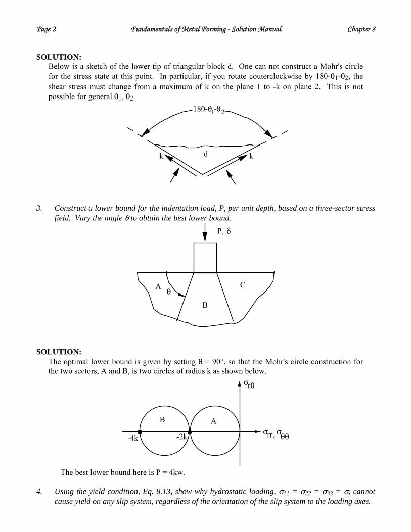
Page 2 Fundamentals of Metal Forming - Solution Manual Chapter 8 SOLUTION:
Below is a sketch of the lower tip of triangular block d. One can not construct a Mohr's circle for the stress state at this point. In particular, if you rotate couterclockwise by 180-θ1-θ2, the shear stress must change from a maximum of k on the plane 1 to -k on plane 2. This is not possible for general θ1, θ2.
kk d
180-θ -θ 1 2
3. Construct a lower bound for the indentation load, P, per unit depth, based on a three-sector stress field. Vary the angle θ to obtain the best lower bound.
P, δ
θA
B
C
SOLUTION: The optimal lower bound is given by setting θ = 90°, so that the Mohr's circle construction for the two sectors, A and B, is two circles of radius k as shown below.
σrr
rθσ
θθσ,-4k -2k
AB
The best lower bound here is P = 4kw.
4. Using the yield condition, Eq. 8.13, show why hydrostatic loading, σ11 = σ22 = σ33 = σ, cannot
cause yield on any slip system, regardless of the orientation of the slip system to the loading axes.

Chapter 8 Fundamentals of Metal Forming - Solution Manual Page 3 SOLUTION:
If the stress state, σ11 = σ22 = σ33 = σ is substituted into the yield condition, Eq.. 8.13, then ± s1
(α)m1(α) + s2
(α)m2(α) + s3
(α)m3(α)( )≥ τc
(α)
or equivalently, ± s(α) ⋅ m(α)( )σ ≥ τc
(α) For slip planes, s and m must be perpendicular to one another, so that s·m = 0 for all slip systems. This statement and the rephrased yield condition above predict that yield can never be reached under hydrostatic loading.
5. Experiments which apply hydrostatic loading to engineering materials have shown that materials such as steel, aluminum, copper, or silicon will yield, although the magnitude of hydrostatic loading to cause yield is many times that required for simple tension or compression. Discuss why materials do yield in hydrostatic loading.
SOLUTION: Typically, engineering grades of materials contain grain boundaries, inclusions, and voids. All serve to act as stress concentrators, so that under nominal hydrostatic loading, the stress state is not homogeneous and entirely hydrostatic. Yield can then occur.
6. A single crystal is indented with a square knife edge as shown below. The candidate slip systems
are oriented at discrete angles θ1, θ2, and θ3.
a. Construct a deformation field out of rigid, sliding triangles, produce the corresponding hodograph, and determine an upper bound to the indentation load.
b. If the crystal had only two slip planes, could you construct a deformation field? Support
your answer with some sketches. What would the indentation load P be under such a case?
m
s
ms
ms
Wθ2=60o θ1=30o
θ3=0o
P
SOLUTION: a. The deformation field and the corresponding hodograph are:

Page 4 Fundamentals of Metal Forming - Solution Manual Chapter 8
C'CD
ww
www
P, v
A
B D'
v2v
3v
v/ 31.5v
v/2
2v/ 3
v/2 3
v/ 3
d
c
a, b
c'
d'
O
The external dissipation rate is Pv. The internal dissipation rate is k[lBC'VBC' + lC'OVC'O + lC'DVC'D + lD'OVD'O +lBCVBC + lCOVCO + lCDVCD + lDOVDO]. Substituting the values for lIJ derived from the deformation diagram and values for vIJ derived from the hodograph, the internal dissipation rate is approximately 6.93 kwv. Equating the external and internal dissipation rates gives: P = 6.93 kw.
b. It is not possible to construct a deformation field to this geometry with only two slip directions, provided that the sample is infinitely thick. Triangular blocks must be constructed for a successful deformation field, and the three sides of the block will require three slip directions.
7. In the upper bound analysis of a block of dimensions l1, l2, and l3, which is sheared by an amount
b along a direction s, on a plane with normal m (see Fig. 8.2), the internal dissipation is IW* = k Ab
and the external dissipation is
EW* = σ11* Abm1s1 + σ22* Abm2s2 where σ11* and σ22* are uniform stresses, and A is the area of slipped plane. a. Sketch the resulting upper bound load to the collapse surfaces in σ11*-σ22* space,
assuming the inclination angle, θ, shown in Fig. 8.2 equals 30°. b. Although the internal strain is concentrated at the slip plane, define an appropriate
average, or macroscopic strain state for the block, after a slip of b has occurred on the plane.
c. Do your macroscopic strains in Part b satisfy normality with the collapse surface in Part
a? Explain why. If they do not propose a definition of macroscopic strain that will satisfy normality.
SOLUTION: a. We note that k = σ11∗m1s1 + σ22*m2s2, where for this problem, m1 = cos 60, s1 = +cos 30, m2 =
cos 30, and s2 = -cos 60. When values of mi and si are substituted into the expression,
Chapter 8 Fundamentals of Metal Forming - Solution Manual Page 5
(σ11∗ - σ22*) = ±43 k
where the ± sign on the RHS is produced by considering positive or negative values of slip on the plane. The result is shown below.
σ11*
σ22*
2.3k
2.3k-2.3k
-2.3k
direction of strain increment
direction of strain increment
(ε )22*
(ε )11*
b. Using Eq. 8.23,
dε- ij = 12
Abl1l2l3 (mjsi + misj)
so that using the particular values for the mi, si,
dε- 11 = ± 34
Abl1l2l3
dε- 22 = m3
4 Ab
l1l2l3
c. The macroscopic strains defined in part (b) do satisfy normality. The strain increments may be
plotted in the σ11*-σ22* diagram in (a), where the ε11* axis is constructed parallel to the σ11* axis, and the ε22* axis is constructed parallel to the σ22* axis. The incremental strains are then at +135°, -45° angles measured counterclockwise from the horizontal axis. They are perpendicular to the yield surface.
8. Construct the projection of the f.c.c. yield surface on to the σ11-σ12 stress plane. Compare your answer to the prediction based on a Tresca yield criterion, σ1 − σ3 = ±2k, where σ1 and σ3 are the maximum and minimum principal stresses, respectively.
SOLUTION:
We note Eq. 8.17 and pick σ1 = σ11 and σ6 = σ12 (=σ21) to be the only non-zero components of stress. The resulting yield condition becomes

Page 6 Fundamentals of Metal Forming - Solution Manual Chapter 8
±16
σ11σ11 + σ12
σ12−σ11 + σ12
−σ12−σ11
−σ11 + σ12σ12σ11σ11
σ11 + σ12σ12
⎡
⎣
⎢ ⎢ ⎢ ⎢ ⎢ ⎢ ⎢ ⎢ ⎢ ⎢ ⎢ ⎢
⎤
⎦
⎥ ⎥ ⎥ ⎥ ⎥ ⎥ ⎥ ⎥ ⎥ ⎥ ⎥ ⎥
≥k
⎡
⎣
⎢ ⎢ ⎢ ⎢ ⎢ ⎢ ⎢ ⎢ ⎢ ⎢ ⎢ ⎢
⎤
⎦
⎥ ⎥ ⎥ ⎥ ⎥ ⎥ ⎥ ⎥ ⎥ ⎥
⎥⎥
Here, the assumption is made that the critical resolved shear stress for each plane is k. The corresponding yield surface is constructed from lines generated from the twelve slip systems represented in the above equation. The corresponding Tresca yield condition is generated from |σ1 - σ3| = 2k. This condition states that the diameter, D, of Mohr's circle, constructed in σ11-σ12 space, can not exceed 2k. The diameter of Mohr's circle for this stress state is
D = 2σ122 + 12 σ112 ( = 2k)
Accordingly, the above is an equation of an ellipse for which the σ11 intercept is ±2k and the σ12 intercept is ±k. It is shown in the figure below.
σ11*
σ22*
6 k
k
2k- 6 k
6 k
- 6 k
9. Imagine that you can load a f.c.c. crystal along any crystallographic direction. Assume that the
potential slip systems are of the type {111}/<110>, as listed in Table 8.1. Find a crystallographic direction along which the tensile stress to yield is a minimum, and report the minimum value of tensile stress in terms of τc, the critical resolved shear stress to activate slip.

Chapter 8 Fundamentals of Metal Forming - Solution Manual Page 7 SOLUTION:
Use the yield condition, Eq. 8.13, expressed in the form, , τ(α) = (s(α) ⋅e(1' ))(m(α) ⋅ e(1' ))σ ≥ ±τc
(α)
where s(α) and m(α) are the slip direction and slip plane normal of slip system (α), and e(1') is the direction along which the tensile stress, σ, is applied. The minimum σ is found by making the factor involving the dot products as large as possible. The largest dot products are obtained by first choosing e(1') to lie in the plane containing s(α) and m(α). Since s(α) and m(α) are orthogonal to each other, the relative orientations of vectors is depicted below, where s(α) · e(1') = sinθ and m(α) · e(1') = cosθ. Therefore,
σ =τc
sin θcosθ ,
and the minimum value, σ = 2τc, occurs when θ = 45°, 135°, 225°, or 315°. There are several possible crystallographic directions of the type e(1')= ±(s(α)±m(α))/ 2 . A possible direction for the {111}/<110> slip systems considered here are [ 2 + 3 2 - 3 2 ]/2 3 .
10. A biaxial stress state is applied to a single crystal of f.c.c. material. However, the crystal is oriented so that one applied stress, σ1'1', is along the [111] crystallographic direction, and the other applied stress, σ2'2', is along the [1-1 0] crystallographic direction. Assume that all slip planes of the type {111}/<110> (see Table 8.1) slip when the critical resolved shear stress reaches τc. Construct a projection of the yield surface onto the σ1'1'-σ2'2' stress plane. Comment on the difference between this projection and the one shown in Fig. 8.4.
SOLUTION:
A relatively simple approach is to revert to the yield condition, Eq. 8.13, and compute directly the resolved shear stress on each of the twelve slip systems according to , τ(α) = (s(α) ⋅e(1' ))(m(α) ⋅ e(1' ))σ1'1' + (s(α) ⋅ e(2' ))(m (α) ⋅ e(2' ) )σ2'2' ≥ ±τc
(α)
where e(1') and e(2') corresponds to the crystallographic directions [111]/ 3 and [1-1 0]/ 2 , and the vectors s(α) and m(α) correspond to the slip directions and slip plane normals, respectively, of slip system (α). The dot products involved project the components of stress, applied along the 1' and 2' directions, on to the s(α) and m(α) directions. The twelve slip systems listed in Table 8.1 are used in the yield condition and produce twelve equations of the form,
σ2'2'6
≥ ±τc (slip systems 7,5)
2σ1'1'3 6
≥ ±τc (slip systems 6,9,11,12)
2σ1'1'3 6
+σ2'2'
6≥ ±τc (slip systems 4,8)
.
The result indicates that two or more slip systems can produce the same yield condition. Slip systems 1, 2, 3, and 10 have zero resolved shear stress on them, and hence, will never yield. The yield surface is depicted by the dotted line in the figure below. For comparison, the

Page 8 Fundamentals of Metal Forming - Solution Manual Chapter 8
projection of the yield surface on to the σ11-σ22 plane is reproduced from Fig. 8.4 and is indicated by the solid line. The differences in yield surfaces demonstrates that yield behavior depends on the choice of loading axes relative to the crystal basis.
6τc
6τc
− 6 τc
6τc−(3, 5, 8, 12)
(1, 6, 9, 10)(2, 4, 7, 11)
(1, 6, 9, 10)
(3, 5, 8, 12)
(2, 4, 7, 11)
(7, 5)
(7, 5)
(6, 9, 11, 12)
(6, 9, 11, 12) (4, 8)
(4, 8)
σ22 or σ2'2'
σ11 or σ1'1'
6τc1.56τc1.5
A more involved approach is to use Eq. 8.17. The components, σi, of stress in that equation refer to the cube basis of the f.c.c. crystal. However, the applied stress is expressed in terms of components along the [111] and [1-1 0] directions. Thus, Eq. 8.17 may be used only if the applied stress state, σ1'1' and σ2'2', is expressed in terms of the components in the crystal basis. Let the basis e(1), e(2), and e(3) correspond to the crystallographic directions, [100], [010], and [001], and the basis e(1') and e(2') corresponds to the crystallographic directions [111]/ 3 and [1-1 0]/ 2 , as before. Then . σ ij = AikA jl ′ σ kl where Aik = e(i) · e(k'), σij corresponds to components in the e(i) basis, and σ'ij corresponds to components in the e(i') basis. Accordingly,
Aik'[ ]=1 / 3 1 / 2 *1 / 3 −1/ 2 *1 / 3 0 *
⎡
⎣
⎢ ⎢
⎤
⎦
⎥ ⎥ ,
and the computed components of stress are
σ1σ2σ3σ4σ5σ6
⎡
⎣
⎢ ⎢ ⎢ ⎢ ⎢
⎤
⎦
⎥ ⎥ ⎥ ⎥ ⎥
≡
σ11σ22σ33σ23σ13σ12
⎡
⎣
⎢ ⎢ ⎢ ⎢ ⎢
⎤
⎦
⎥ ⎥ ⎥ ⎥ ⎥
=σ1'1'
3+
σ2'2'2
11000−1
⎡
⎣
⎢ ⎢ ⎢ ⎢ ⎢
⎤
⎦
⎥ ⎥ ⎥ ⎥ ⎥
.
Substitution into Eq. 8.17 produces the same three types of yield conditions derived from the first approach.
11. A sphere with radius r = 1cm is a single f.c.c. crystal. Slip systems 1, 6, and 12 listed in Table 8.1

Chapter 8 Fundamentals of Metal Forming - Solution Manual Page 9
are activated, so that a slip of 1μm in the corresponding +s directions listed occurs on slip planes which pass right through the center of the sphere. Calculate the resulting macroscopic strain in the crystal.
SOLUTION:
The resulting macroscopic strain is given by
ε ij =12α
∑ As(α)b(α)
Vmi
(α)s j(α) + mj
(α)si(α)( )
where the sum α is over slip systems 1, 6, and 12. The slip area As = πr2 and the amount of slip b(α) = 1μm for the three slip systems. Also, V = 4πr3/3, where r = 1 cm. Consequently, the equation for average strain above yields contributions for each of the three active slip systems,
ε ij =3
8 6⋅10−4 m jsi + mis j( )(1)
+ m jsi + mis j( )(6)+ m jsi + mis j( )(12)⎡
⎣ ⎤ ⎦
Substituting values of mj and si for each of the slip systems, ε ij[ ]=3
8 6⋅10−4
0 1 31 2 03 0 −2
⎡
⎣
⎢ ⎢
⎤
⎦
⎥ ⎥
12. Consider the portion of the yield surface in Fig. 8.4 that is contributed by slip systems 2, 4, 7, and
11. Using Eq. 8.25, show that operation of any individual or linear combination of these slip systems produces a strain increment which is perpendicular to that portion of the yield surface shown in the figure.
SOLUTION:
The relevant equation is ε ij =dγ (α)
2α∑ mis j + m jsi( )(α)
Applying this to slip systems 2 and 11, we find dε 11(α) =
dγ (α)
6, dε 22
(α) = 0
and applying this to slip systems 4 and 7, dε 11(α) = −
dγ (α)
6, dε 22
(α) = 0 .
Since each individual system produces zero dε22, any linear combination of operation of these slip systems will do the same. When plotted in ε11-ε22 space, the strain increment is perpendicular to the yield surface lines contributed by slip systems 2, 4, 7, and 11 in Fig. 8.4. Note that components of strain other than ε11 may be non-zero here, but that the projected strain increment in ε11-ε22 space is still normal to the yield surface in σ11-σ22 space shown.
13. Equation 8.24 states that external and internal plastic work increments are equal. Show that this
equation may be converted to the notation, σidεi = , where the components [σi] = [σ1, σ2, σ3, σ4, σ5, σ6] = [σ11, σ22, σ33, σ23, σ13, σ12], and the components [dεi] are defined by the identity, Eq. 8.31.
(τcdγ )(α)�
SOLUTION:

Page 10 Fundamentals of Metal Forming - Solution Manual Chapter 8
Equating internal and external plastic work increments produces σ ijdεij = τc(α)dγ (α)
(α)∑
or if the contracted notation σi, dεi is used, then the following must hold for each slip system (α) . σidεi
(α) = τc(α)dγ (α)
Equilibrium requires that the stress state produces a resolved shear stress on each active slip system such that
τc(α) = σ1 m1s1( )(α) + σ2 m2s2( )(α) + σ3 m3s3( )(α)
+σ4 m2s3 + m3s2( )(α)
+σ5 m1s3 + m3s1( )(α)
+σ6 m1s2 + m2s1( )(α)
When this is used to replace τc(α) in Eq. (*) above, then there equivalence of work only if
dε1(α) = m1s1( )(α)dγ (α)
dε2(α) = m2s2( )(α) dγ (α)
dε3(α) = m3s3( )(α)dγ (α)
dε4(α) = m2s3 + m3s2( )(α)dγ (α)
dε5(α) = m1s3 + m3s1( )(α) dγ (α)
dε6(α) = m1s2 + m2s1( )(α)dγ (α)
Eq. 8.31 is shown using the correspondence above and invoking that
dεij(α) =
dγ (α)
2mjsi + misj( )(α)
.
14. Use Eq. 8.25 to show that no combination of slip systems can produce dilatation. SOLUTION:
Eq.. 8.25 states that dεij =dγ (α)
2mjsi + misj( )(α)
α∑ .
Since dε11 + dε22 + dε33 is the incremental volume change per unit volume, the above relation is used to find the volume change associated with activated slip systems,
dε11 + dε22 + dε33 = dγ (α) m1s1 + m2s2 + m3s3( )(α)
α∑
= dγ (α) m(α) ⋅α∑ s(α)
.
Since m·s = 0 for each slip system α, the above relation indicates that dε11 + dε22 + dε33 = 0.
15. Of the twelve slip systems listed in Table 8.1, choose slip systems 1, 2, and 6. Determine whether

Chapter 8 Fundamentals of Metal Forming - Solution Manual Page 11
these 3 slip systems are independent.
SOLUTION: Using Eq. 8.23, the respective strain increments contributed by slip systems 1, 2, and 6 in Table 8.1 are
ε ij(1) =
dγ (1)
2 6
2 0 10 −2 −11 −1 0
, ε ij(2) =
dγ (1)
2 6
2 1 01 0 −10 −1 −2
, ε ij(6) =
dγ (1)
2 6
−2 0 10 2 11 1 0
. or equivalently, the short-hand notation, dεi(α)=dγ(α)ni(α), from Eq. 8.22 may be used, where the ni(α) are determined according to Eq. 8.16,
ni(1)[ ]=
16
1−10−110
⎡
⎣
⎢ ⎢ ⎢ ⎢ ⎢
⎤
⎦
⎥ ⎥ ⎥ ⎥ ⎥
ni(2)[ ]=
16
10−1−101
⎡
⎣
⎢ ⎢ ⎢ ⎢ ⎢
⎤
⎦
⎥ ⎥ ⎥ ⎥ ⎥
ni(6)[ ]=
16
−110110
⎡
⎣
⎢ ⎢ ⎢ ⎢ ⎢
⎤
⎦
⎥ ⎥ ⎥ ⎥ ⎥
.
The systems are linearly independent if no values of x and y can satisfy xεij(1) + yεij(2) = εij(6), for all components ij, or equivalently, if no values of x and y can be found that satisfy xni(1) + yni(2) = ni(6) for all components i. After some examination, x = -1 and y = 0 appear to satisfy the above relations for all components except dε13 (or equivalently, dε5). Accordingly, these three slip systems are independent, since no combination of x and y can be found to satisfy the above relations.
16. Suppose you load in tension along the [3 8 6] direction in a f.c.c. material in which the candidate slip systems are of the type listed in Table 8.1. The crystal begins to yield at a tensile stress of 10MPa. Assume that all slip systems require the same critical resolved shear stress, τc, for activation. What slip system will be activated first? What is the value of τc? To what crystallographic direction will the tensile axis rotate? What is the axis about which the tensile axis rotates?
SOLUTION:
The yield condition, Eq. 8.13, can be used to determine that slip system 6 in Table 8.1 will require the smallest tensile stress to activate it. The yield condition for that slip system is stated as
[110]2
⋅[386]
109⎛ ⎝
⎞ ⎠
[−111]3
⋅[386]
109⎛ ⎝
⎞ ⎠ 10MPa = τc .
so that τc to yield is approximately 4.5MPa. As indicated in Eq. 8.37, the tensile axis will rotate toward the slip direction, [110]. The direction, r, about which the rotation occurs is given by T∞s, so that r is parallel to [-6 6 -5].

Page 12 Fundamentals of Metal Forming - Solution Manual Chapter 8
17. Derive the results,
Ý β = −Ý b
Ho sin βosin2 β
Ý β = − Ý ε TTsin βcos β
by analyzing the 2D slip plane geometry below, where Ý b and Ý ε TT are the increment in slip on the plane and average strain increment parallel to the current tensile axis, respectively. The other parameters are labeled in the sketch. Do not use the general formulation associated with the discussion of Fig. 8.5(a,b), but rather, derive the expression from a trigonometric analysis of the 2-D geometry below.
kk d
180-θ -θ 1
σ
m s
T
σ
s
m
T
β
Ho
2βo
SOLUTION:
The geometry below is used, and application of the law of sines produces
Hsin(180 − βo)
=Ho
sinβb
sin(βo −β)=
Hosinβ
s
H
o180-β β
Ho
TTo
Noting that sin(βo-β) = sinβocosβ - cosβοsinβ and differentiating the second relation,
Chapter 8 Fundamentals of Metal Forming - Solution Manual Page 13
Ý b = −H o sinβo
sin2 βÝβ
Differentiate the first relation and then divide each side by the originating terms in the first relation. Substitute Ý H / H = Ý ε TT to get
Ý β = −sinβcosβ
Ý ε TT .
18. Eq. 8.56 defines the increment, dεij*, in components of strain that are expressed in the reference
coordinate system. Derive this relation, beginning with a statement of the Principle of Virtual Work that σij*dεij* = ∑τ(β)dγ(β) .
SOLUTION:
We begin with a statement of the Principle of Virtual Work, τ(β )∑ dγ (β ) = σij*dεij
* .
and note from Eq. 8.48 that since σij* = σji*, then τ (β ) =12
σij* si
*(β )mj*(β ) + sj
*(β )mi*(β )( ) .
If the expression for τ(β) is substituted in the statement of the Principle of Virtual Work, then dεij* must be defined according to Eq. 8.56.
19. Suppose you have a similar geometry as in Problem 11, but instead, there are two competing slip systems, (m(1), s(1)) and (m(2), s(2)). βo is the initial angle between s(1) and the initial tensile axis direction, To, and γo is the corresponding initial angle for slip system (2).
Suppose you have documented the angle β as a function of macroscopic strain, εTT, along the T
(not To!) axis. Explain how you could determine the relative amount of slip, b(1) and b(2), on each system. Do you have enough information?
SOLUTION:
First, we note the assumption that all m(α) and s(α) for both systems are coplanar with T and use the geometry below.
Page 14 Fundamentals of Metal Forming - Solution Manual Chapter 8
H
β
Ho
TTo
s (1)
(2)s
o
βs (1)
γob
First, note that Ý H = Ý b (1) cosβ + Ý b (2) cos γÝ β = Ý γ
The second condition is holds since the lattice rotates rigidly, relative to the T axis. Also note that
Hcos(β − βo) = Ho + b(1) cosβo + b(2) cosγ o
Hsin(β − βo) = b(1) sinβo + b(2) sin γ o Each of these relations may be divided through by Ho, any occurrence of H/Ho in these relations may be replaced by exp(ε- TT),. The two equations relate the two unknowns, b(1)/Ho and b(2)/Ho, to the current tensile strain, ε- TT, the starting angles γo and βo, and the current angle β. Final expressions are left to the reader to derive.
20. Consider a material in which the critical resolved shear stress to shear a plane with normal m(α) depends on the stress normal to the plane, according to
τc(α) = τo − μf mi
(α)σijm j(α)( )
where τo is the critical resolved shear with zero normal load, and μf is a coefficient of friction.
Such behavior is consistent with a hard sphere atomic picture of materials, in which the activation barrier to slide particles past one another increases with confining pressure on the material. Show that when a macroscopic stress with non-zero components σ11 and σ22 is applied, the yield condition for a slip system (α) with slip direction s(α) and slip plane normal m(α) is
±s1(α) + μ f m1
(α)( )m1(α)σ11 + ±s2
(α) + μ fm2(α)( )m2
(α)σ22 ≥ τo where ± must be interpreted as either + for both terms (+s1(α) and +s2(α)) or - for both terms (-
s1(α) and -s2(α)).
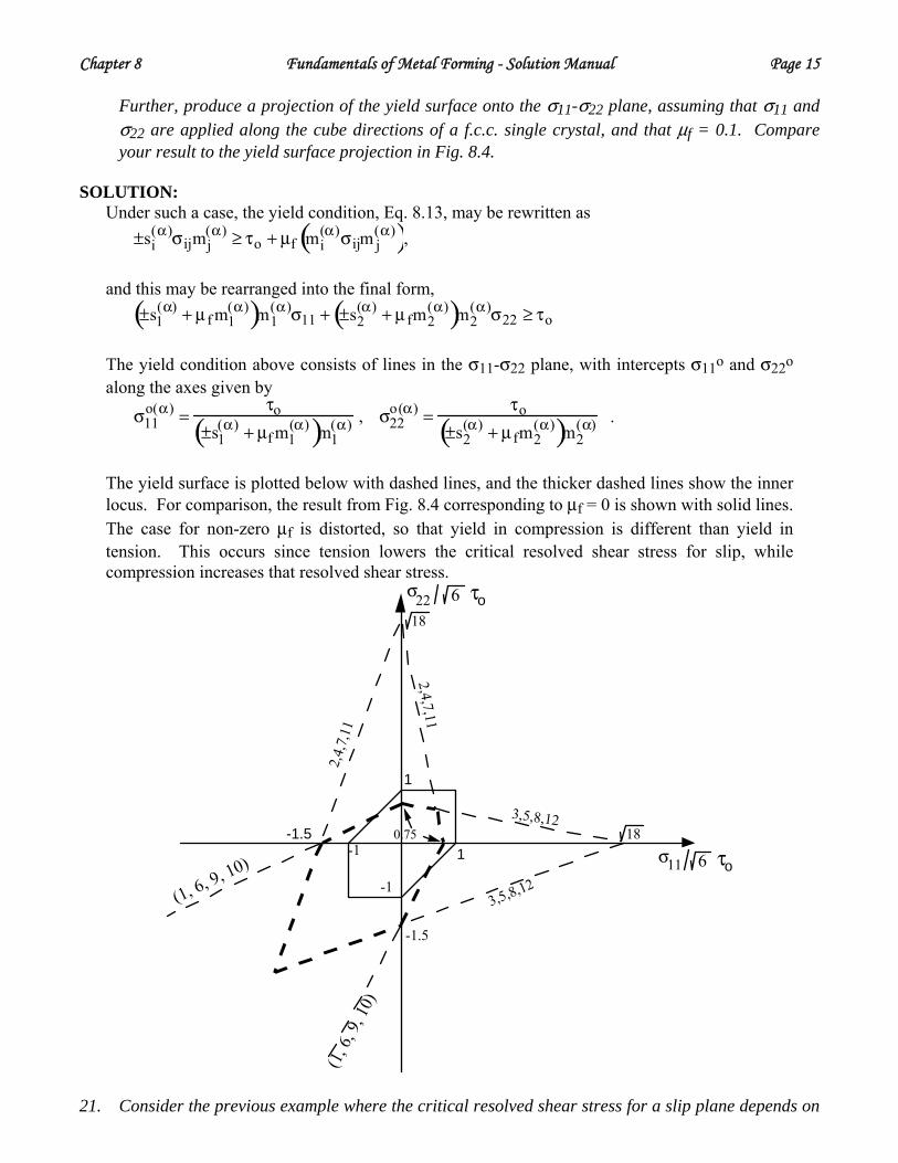
Chapter 8 Fundamentals of Metal Forming - Solution Manual Page 15 Further, produce a projection of the yield surface onto the σ11-σ22 plane, assuming that σ11 and
σ22 are applied along the cube directions of a f.c.c. single crystal, and that μf = 0.1. Compare your result to the yield surface projection in Fig. 8.4.
SOLUTION:
Under such a case, the yield condition, Eq. 8.13, may be rewritten as ±si
(α)σijmj(α) ≥ τo + μf mi
(α)σijm j(α)( ),
and this may be rearranged into the final form, ±s1
(α) + μ f m1(α)( )m1
(α)σ11 + ±s2(α) + μ fm2
(α)( )m2(α)σ22 ≥ τo
The yield condition above consists of lines in the σ11-σ22 plane, with intercepts σ11o and σ22o along the axes given by
σ11o(α) =
τo±s1
(α) + μf m1(α)( )m1
(α) , σ22o(α) =
τo±s2
(α) + μ fm2(α)( )m2
(α) .
The yield surface is plotted below with dashed lines, and the thicker dashed lines show the inner locus. For comparison, the result from Fig. 8.4 corresponding to μf = 0 is shown with solid lines. The case for non-zero μf is distorted, so that yield in compression is different than yield in tension. This occurs since tension lowers the critical resolved shear stress for slip, while compression increases that resolved shear stress.
(1, 6
, 9, 1
0)
(1, 6, 9, 10)
σ22
σ11
2,4,7,11
2,4,
7,11
3,5,8,12
3,5,8,126 τo
6 τo
1-1.5 18
1
0.75
18
-1.5
-1
-1
21. Consider the previous example where the critical resolved shear stress for a slip plane depends on
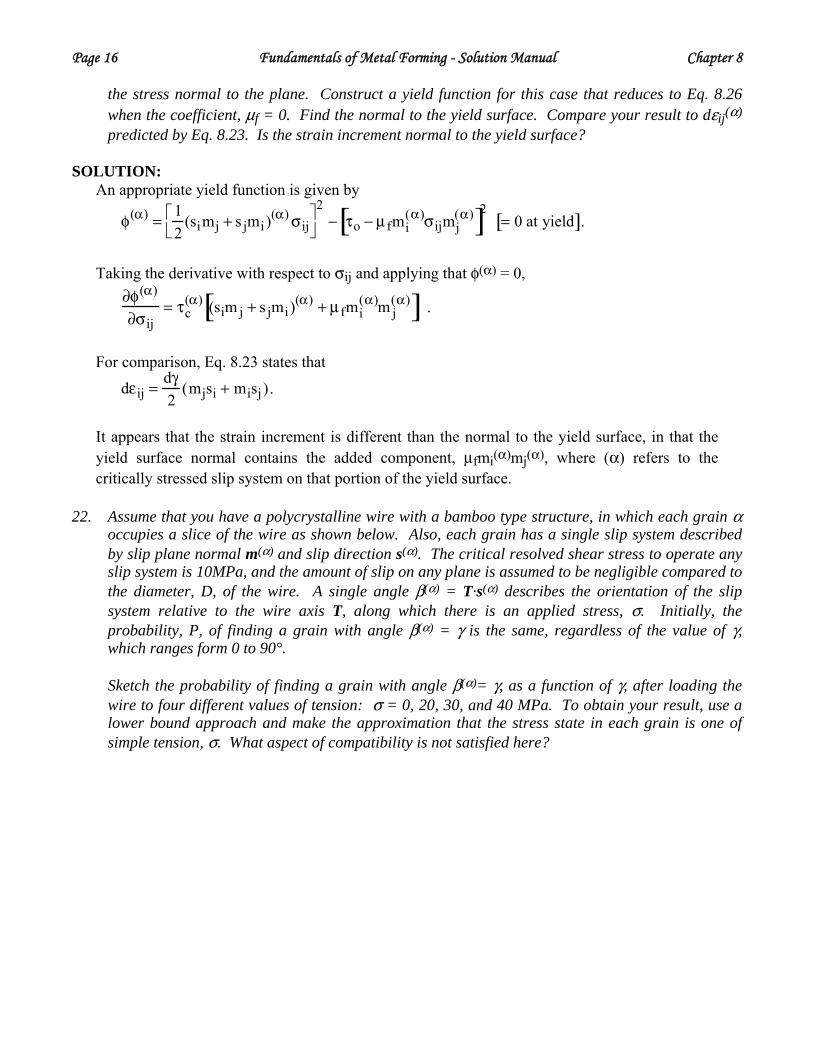
Page 16 Fundamentals of Metal Forming - Solution Manual Chapter 8
the stress normal to the plane. Construct a yield function for this case that reduces to Eq. 8.26 when the coefficient, μf = 0. Find the normal to the yield surface. Compare your result to dεij(α) predicted by Eq. 8.23. Is the strain increment normal to the yield surface?
SOLUTION:
An appropriate yield function is given by
φ(α) =12
(simj + s jmi)(α) σij
⎡ ⎣
⎤ ⎦
2− τo − μ fmi
(α)σijmj(α)[ ]2 = 0 at yield[ ].
Taking the derivative with respect to σij and applying that φ(α) = 0,
∂φ(α)
∂σij= τc
(α) (sim j + s jmi)(α) + μ fmi
(α)m j(α)[ ] .
For comparison, Eq. 8.23 states that
dεij =dγ2
(mjsi + misj ).
It appears that the strain increment is different than the normal to the yield surface, in that the yield surface normal contains the added component, μfmi(α)mj(α), where (α) refers to the critically stressed slip system on that portion of the yield surface.
22. Assume that you have a polycrystalline wire with a bamboo type structure, in which each grain α occupies a slice of the wire as shown below. Also, each grain has a single slip system described by slip plane normal m(α) and slip direction s(α). The critical resolved shear stress to operate any slip system is 10MPa, and the amount of slip on any plane is assumed to be negligible compared to the diameter, D, of the wire. A single angle β(α) = T·s(α) describes the orientation of the slip system relative to the wire axis T, along which there is an applied stress, σ. Initially, the probability, P, of finding a grain with angle β(α) = γ is the same, regardless of the value of γ, which ranges form 0 to 90°.
Sketch the probability of finding a grain with angle β(α)= γ, as a function of γ, after loading the
wire to four different values of tension: σ = 0, 20, 30, and 40 MPa. To obtain your result, use a lower bound approach and make the approximation that the stress state in each grain is one of simple tension, σ. What aspect of compatibility is not satisfied here?

Chapter 8 Fundamentals of Metal Forming - Solution Manual Page 17
D
T
σ
σ SOLUTION:
The assumption that the stress state in each crystal is simple tension violates compatibility across the grain boundaries in the bamboo structure. To begin, we sketch that the probability P of finding a grain with a certain angle β(α) is uniform, and since β may span from 0 to 90°, the initial probability must be 1/90 for all possible angles. This is sketched below and labeled σ = 0, 20 MPa. The analysis for other levels of stress is done by imposing that each grain that meets or exceeds the yield condition will continue to strain, and therefore rotate until the yield condition is exceeded. When the tensile stress is 20MPa, then we check for any grain orientation angle β for which the resolved shear stress exceeds 10MPa, i.e., for which τ = 20MPa cosβ sin β ≥ τc (= 10MPa) The yield condition above is just met for any grain at angle 45°. As soon as rotation occurs, so that β = 45°-Δβ, the rotation stops, for the yield condition is no longer met. Therefore, at a tensile stress of 20MPa, grains with orientation angle β = 45° just meet the yield criterion. The rotation is negligible at this point, assuming that τc remains at 10MPa even after slip is activated. At a tensile stress of 30MPa, the yield condition is stated as: 30 MPa ⋅ cos β ⋅ sin β ≥ 10 MPa Therefore, yield is exceeded for all grains with β in between 21° and 69°. All such grains continue to rotate until β = 21°. Thus, in a bamboo structure with 90 grains (and equally distributed with angle), 48 of those grains would displace to the 21° position, for a total probability of 49 grains out of 90 having an angle β = 21°, zero probability for β in between 21° and 69°, and P = 1/90 for all other angles. At a tensile stress of 40MPa, the yield condition reveals that all grains with initial angles between 15° and 75° must rotate to the 15° position. Therefore, the probability is P = 61/90 at β = 15°, zero for all angles between 15° and 75°, and P = 1/90 for all other angles. The results are summarized in the figure below.

Page 18 Fundamentals of Metal Forming - Solution Manual Chapter 8
0 30 60 90
P = Probability of finding a grain with angle β +/- 0.5
1/90
47/90
60/90
15 21 69 75
σ= 0, 20MPa
σ= 30MPa
σ= 40MPa
o
orient. angle β 23. Outline the components of a computer program which will calculate the uniaxial stress-strain
response of a f.c.c. single crystal loaded in tension. The tensile axis T is a material one, similar to the case depicted in Fig. 8.5, and initially, T is parallel to [1 12 11]. The sample is loaded from 0 to 40MPa over a period of 300s, so that the stress rate, dσTT/dt is constant. Use a rate-dependent constitutive relation as described in Eqs. 8.73 and 8.74 with the following parameters:
Ý γ o(α ) = 10−3 / s
m = 20
τo(α ) = 10MPa (initially, prior to any slip)
Case A: hαβ =0MPa if α = β5MPa if α ≠ β⎧ ⎨ ⎩
Case B: hαβ =5MPa if α = β0MPa if α ≠ β⎧ ⎨ ⎩
Note that Case A simulates a larger latent hardening situation, and Case B simulates a larger self
hardening situation. Produce for each case the tensile stress-tensile strain curves along T, from εTT= 0 to
approximately 0.8. Note the direction of T in each case when εΤΤ = 0.8. For each case, discuss the dominant slip system(s) when εΤΤ = 0 and when εΤΤ = 0.8.
SOLUTION: The generic outline of the computer program is to
• define the time increment, Δt, to be sufficiently small, e.g., Δt=0.01s • define the tensile loading rate, dσTT/dt = 40MPa/300s.
• initialize τo(α) = 10MPa. • define the unit vector T along the tensile axis to be parallel to [1 12 11]. In general, the
components of all quantities will be referred to the crystal basis rather than the reference (*) basis containing T.
• define all twelve sets of mi(α) and si(α) according to Table 8.1.

Chapter 8 Fundamentals of Metal Forming - Solution Manual Page 19
• define the components hαβ of the 12 by 12 matrix according to either of the two cases mentioned. For case A, hαβ = 5MPa if α ≠ β, and hαβ = 0 if α = β. For case B, hαβ = 0 if α ≠ β, and hαβ = 5MPa if α = β.
• begin an outer loop in which the time is incremented by Δt until the strain along the tensile axis exceeds 0.80. In this loop...
-increment σTT by Δt(dσTT/dt). -compute all τ(α) according to Eq. 8.13, or equivalently, τ (α ) = σTT s(α ) ⋅T( )m(α ) ⋅ T( ) . -calculate the increment,
dγ (α ) =10−3
sτ (α )
τo(α )
⎛
⎝ ⎜
⎞
⎠ ⎟
20
Δt .
-compute the components, dT = dγ (α ) m(α) ⋅ T( )∑ s(α) − s(α ) ⋅ T( )T{ } .
-in order to define the strain increment, dεTT, first compute the work,
dw = ∑|τ(α)dγ(α)| , and then define
dεTT =dwσTT
.
-update the total strain according to εTT = εTT + dεTT -update T according to Ti = Ti + dTi
-update the τo(α) according to τo(α) = τo(α) + ∑hαβdγ(β) -print out εTT, σTT.
• end the outer loop Results for Case A (larger latent hardening) and Case B (larger self hardening) are shown below. The tensile flow stress for the larger self hardening case is larger, particularly at larger strains. For both cases, slip system 6 in Table 8.1 has the larger resolved shear stress initially, and slip systems 1 and 4 have the second largest. This can be verified by noting in Fig. 8.6 that slip system 6 has the largest resolved shear stress when the tensile axis is in the vicinity of point P. For the larger latent hardening case (A), slip system 6 has the largest slip increment, dγ(α) over the entire range considered, from εTT = 0 to 0.8. In contrast, the larger self hardening case (B) displays several transitions, and at εTT = 0 to 0.8, slip system 4 has the largest slip increment. For Case A, the components of T at εTT = 0.8 are approximately [0.51 0.80 0.31], and T continues to rotate toward [1 1 0]. However, the corresponding components for Case B are approximately [0.49 0.65 0.58]. The larger self hardening in Case B causes the slip system with the largest current dγ(α) to harden substantially, so that no one slip system dominates over the entire history of loading.

Page 20 Fundamentals of Metal Forming - Solution Manual Chapter 8
0
5
10
15
20
25
30
35
40
45
0 0.1 0.2 0.3 0.4 0.5 0.6 0.7 0.8 0.9
stre
ss a
long
tens
ile a
xis
(MP
a)
strain along tensile axis
hself>hlatent
hself<hlatent
Strain along tensile axis
Stre
ss a
long
tens
ile a
xis (
MPa
)
24. Consider a polycrystal with random orientation of crystals. Produce a lower bound to yield in
tension. SOLUTION:
The simplest lower bound is to assume a trial stress distribution that is a homogeneous, simple tension state, and that does not violate yield at any point in the material. In that case, In that case, Eq. 8.42 indicates that the largest tensile stress possible is 2τc, corresponding to some optimally oriented slip system that is with m · T = s · T = 1/ 2 . Here, τc corresponds to the critical resolved shear stress to activate that slip system.

CHAPTER 9 - PROBLEM SOLUTIONS A. PROFICIENCY PROBLEMS 1. For the geometry shown in Fig. 9.1b, find the relationship between the friction coefficient and the
ramp angle at which sliding begins. SOLUTION: The equilibrium of forces is projected on the x and y axes of the figure below.
w
fT
fN
y
xθ
x direction: w sinθ - fT = 0y direction: - w cosθ + fN = 0Or: fT = w sinθ
fN = w cosθ
From the Coulomb friction law we obtain:
μ =
fF
fN=
w sin θw cos θ
= tanθ (at the start of motion)
2. Use the rope formula to obtain the unknown forces in each of the following cases, assuming a
friction coefficient of μ = 0.2.
100N
F
100N
F
(a) (b)1motion
motion
100N
(c)
1/2
motion
100N
1/2
1 (d)
motion
F
F
100N
-1 1
F
(e)
motion
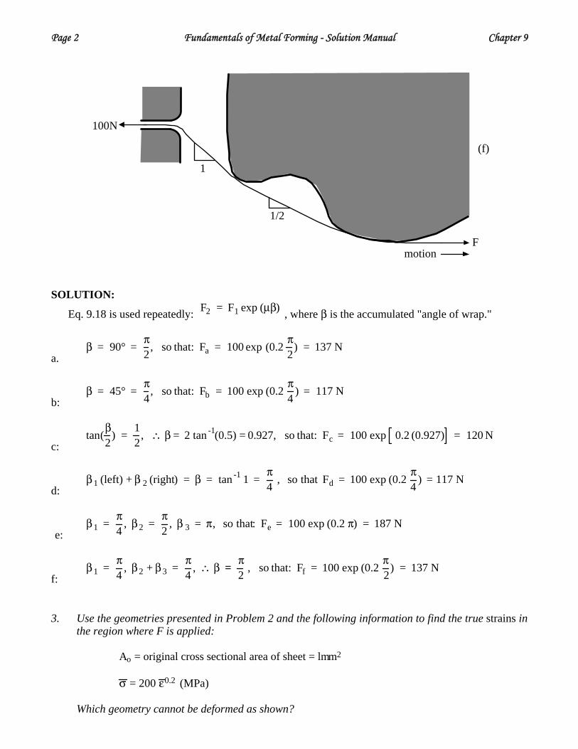
Page 2 Fundamentals of Metal Forming - Solution Manual Chapter 9
1/2
1
100N
F
(f)
motion
SOLUTION:
Eq. 9.18 is used repeatedly: F2 = F1 exp (μβ) , where β is the accumulated "angle of wrap."
a. β = 90° =
π2
, so that: Fa = 100 exp (0.2π2
) = 137 N
b: β = 45° =
π4
, so that: Fb = 100 exp (0.2π4
) = 117 N
c: tan(
β2
) =12
, ∴ β = 2 tan -1(0.5) = 0.927, so that: Fc = 100 exp 0.2 (0.927) = 120 N
d: β 1 (left) + β 2 (right) = β = tan -1 1 =
π4
, so that Fd = 100 exp (0.2π4
) = 117 N
e: β 1 =
π4
, β 2 =π2
, β 3 = π, so that: Fe = 100 exp (0.2 π) = 187 N
f: β 1 =
π4
, β 2 + β 3 =π4
, ∴ β =π2
, so that: Ff = 100 exp (0.2π2
) = 137 N
3. Use the geometries presented in Problem 2 and the following information to find the true strains in the region where F is applied:
Ao = original cross sectional area of sheet = lmm2
σ = 200 ε0.2 (MPa) Which geometry cannot be deformed as shown?

Chapter 9 Fundamentals of Metal Forming - Solution Manual Page 3 SOLUTION:
First, calculate the maximum force which can be applied to the strip without breaking it, assuming a uniaxial tensile state of stress (see Chapter 1):
F = σ A = 200 MPA = N
mm2 ε0.2 1mm2 exp(- ε)
σ A The maximum force occurs at ε = n = 0.2:
Fmax = 200 MPA = Nmm2 0.20.2 1mm2 exp (- 0.2) = 119 N
The rope will not break only for cases b and d. For these cases, the strains may be calculated (by trial-and-error or Newton iteration, for example) as follows:
Fb or d = 117 = 200 exp(-ε) ε0.2 ⇒ ε = 0.13
4. a. A ring compression test is carried out using a standard forging press. The original and final ring dimensions are shown below. Find the value of m or μ from these data using Fig. 9.14.
Height (original) = 100mm Height (final) = 60mm Inside radius (original) = 200mm Inside radius (final) = 160mm b. Given the purpose and use of the ring compression test, which limiting form of friction (Coulomb
or sticking) is likely to be the more accurate? SOLUTION: a. The height and radius reductions are:
Δhh
= 100 - 60100
= 40%
Δriri
= 200 - 160200
= 20%
These values allow the use of Fig. 9.14 to determine the friction factors: for a Coulomb friction law: μ ≅ 0.25 for a sticking friction or Tresca law: m ≅ 1.
b. Direct compression will involve contact pressures near the flow strength of the material. Then, according to our simple view of friction regimes, Fig. 9.3, the friction is likely to follow more closely a sticking friction or Tresca model. To verify which friction law is more accurate, several tests should be carried out with different reduction ratios in height. With these tests, one will be able to see if the experimental measurements on the evolution of the radii follow a curve

Page 4 Fundamentals of Metal Forming - Solution Manual Chapter 9
generated by assuming either of the models presented in Fig. 9.14. 5. What are the friction factors determined for solid soap, graphite in heavy way oil, and way oil
from Fig. 9.16? What difficulty do you see in applying this test to differentiate lubricant properties for production applications?
SOLUTION:
In Fig. 9.16 we observe that: - solid soap corresponds to m = 0.1 at the beginning of the process and m = 0.05 after; - graphite in heavy way oil follows rather well the curve with m = 0.1; - heavy way oil is closer in average to the m = 0.2 curve. This test is not selective enough for a classification of the industrial lubricants, particularly at the beginning of the process.
6.a. For the double-backward extrusion test, the test is stopped at two punch strokes and the cups
removed. Given the following experimental results and using Fig. 9.18, determine the friction coefficients and friction factors for this case.
Punch stroke = 100mm, h1 = 80mm, h2 = 30mm Punch stroke = 200mm, h1 = 120mm, h2 = 90mm b. What can you say about the role of sliding distance in determining friction for this configuration,
lubricant, and material combination? SOLUTION: a. For a punch stroke of 100 mm we have (using Fig. 9.18):
h1h2
= 80300
= 2.67 so that m ≅ 0.15
and for a punch stroke of 200 mm:
h1h2
= 12090
= 1.33 so that m ≅ 0.08
b. The sliding distance is approximately constant in this test as the radii of the punches decrease so
that the contact with the part takes place on a small area and not on the extruded length.
B. DEPTH PROBLEMS 7. Derive an equation or equations that could be solved numerically to find ε1 or ε2 as a function of
H for the test shown in the figure. Assume Coulomb friction, Hollomon hardening ( ), and uniform tensile strain (and tensile stress) in each leg. For simplicity, assume that the pins have negligible diameter, so that the geometry can be computed simply.
σ = k εn
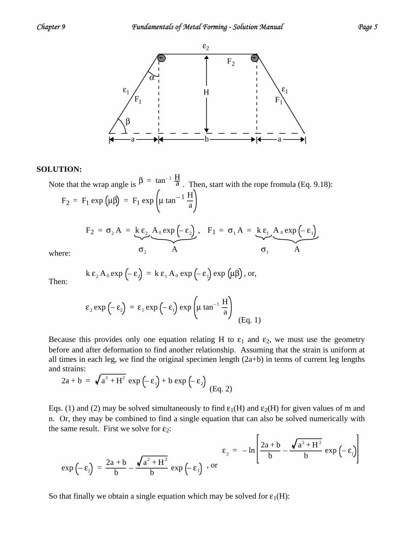
Chapter 9 Fundamentals of Metal Forming - Solution Manual Page 5
ε2
H
α
β
ε1 ε1F1 F1
F2
a b a
SOLUTION:
Note that the wrap angle is β = tan– 1 H
a . Then, start with the rope fromula (Eq. 9.18):
F2 = F1 exp μβ = F1 exp μ tan– 1 H
a
where:
F2 = σ2 A = k ε2 A 0 exp – ε2 , F1 = σ1 A = k ε1 A 0 exp – ε1
σ2 A σ1 A
Then: k ε2 A 0 exp – ε2 = k ε1 A 0 exp – ε1 exp μβ , or,
ε2 exp – ε2 = ε1 exp – ε1 exp μ tan– 1 H
a (Eq. 1)
Because this provides only one equation relating H to ε1 and ε2, we must use the geometry before and after deformation to find another relationship. Assuming that the strain is uniform at all times in each leg, we find the original specimen length (2a+b) in terms of current leg lengths and strains:
2a + b = a2 + H2 exp – ε1 + b exp – ε2
(Eq. 2) Eqs. (1) and (2) may be solved simultaneously to find ε1(H) and ε2(H) for given values of m and n. Or, they may be combined to find a single equation that can also be solved numerically with the same result. First we solve for ε2:
exp – ε2 =
2a + bb –
a2 + H 2
b exp – ε1 , or
ε2 = – ln2a + b
b–
a2 + H 2
bexp – ε1
So that finally we obtain a single equation which may be solved for ε1(H):
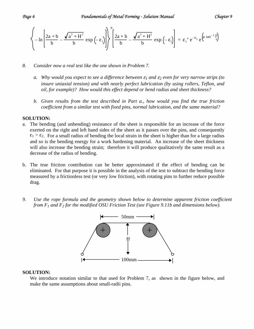
Page 6 Fundamentals of Metal Forming - Solution Manual Chapter 9
– ln2a + b
b–
a2 + H 2
bexp – ε1
n
2a + bb
–a2 + H2
bexp – ε1 = ε1
n e– ε1 eμ tan– 1 H
a
8. Consider now a real test like the one shown in Problem 7.
a. Why would you expect to see a difference between ε1 and ε2 even for very narrow strips (to insure uniaxial tension) and with nearly perfect lubrication (by using rollers, Teflon, and oil, for example)? How would this effect depend or bend radius and sheet thickness?
b. Given results from the test described in Part a., how would you find the true friction
coefficient from a similar test with fixed pins, normal lubrication, and the same material? SOLUTION: a. The bending (and unbending) resistance of the sheet is responsible for an increase of the force
exerted on the right and left hand sides of the sheet as it passes over the pins, and consequently . For a small radius of bending the local strain in the sheet is higher than for a large radius
and so is the bending energy for a work hardening material. An increase of the sheet thickness will also increase the bending strain; therefore it will produce qualitatively the same result as a decrease of the radius of bending.
ε1 > ε2
b. The true friction contribution can be better approximated if the effect of bending can be
eliminated. For that purpose it is possible in the analysis of the test to subtract the bending force measured by a frictionless test (or very low friction), with rotating pins to further reduce possible drag.
9. Use the rope formula and the geometry shown below to determine apparent friction coefficient from F1 and F2 for the modified OSU Friction Test (see Figure 9.11b and dimensions below).
50mm
H
100mm SOLUTION:
We introduce notation similar to that used for Problem 7, as shown in the figure below, and make the same assumptions about small-radii pins.

Chapter 9 Fundamentals of Metal Forming - Solution Manual Page 7
H
ab
a
α
β
ε1 ε1
F'
F2
F1/2
F2
F1/2
F'
F1/2
F'
F2
F' / sin ββ
The equilibrium of vertical forces and the rope formula provide two equations relating F1, F2, and F':
F ′ sin β =
F1
2 , F ′ = F2 exp (μβ)
where, as in Problem 7, β = tan– 1 H
a . F' is then eliminated from the equations, which are solved for μ to obtain the desired expression:
μ =1β ln
12 sin β
F1
F2=
lnH2 + a2
2 HF1F2
tan -1 Ha
10. a. Explain qualitatively why and how the friction factor or friction coefficient affects the shape change in the ring compression test.
b. Could you design a plane-strain compression test similar to the ring compression test by simply putting a long square rod between flat platens?
SOLUTION: a. For a very low friction factor, the solution of the ring upsetting problem corresponds to a
homogeneous strain, so that the ratio between the inner and the outer radii will remain constant. On the other hand, when the friction stress cannot be neglected, its effect will be more important on the large radius zone because of the fact that it is exerted on a larger surface and the velocity is higher. The braking effect of friction is therefore more important on the outer radius than on the inner one. That is why the inner radius increases relatively slower than the outer one, and in fact decreases for large friction stress.
b. If the rod is sufficiently long, a zero-displacement boundary condition will be enforced by friction in the long direction. Then, we could watch the growth of the central or contact width as a function of H, or the ratio of the central width to contact width. For higher friction, the contact width will increase less relative to the central width (i.e. "barreling" will be promoted).

CHAPTER 10 - PROBLEM SOLUTIONS A. PROFICIENCY PROBLEMS 1. Calculate the ideal work to strain a unit volume of material under uniaxial tension from
ε = 0 to ε = ε for each of the following hardening laws:
a. σ = K (ε + εo)n (Ludwik law)
b. σ = σo + K (ε + εo)n (Swift law)
c. σ = σo (1- A e-βε) (Voce law)
d. σ = K (ideal plastic)
e. σ = σo + Kε (linear hardening) SOLUTION:
a.
wv = dw
o
ε= σdε = K ε + εo
n
o
εdε
o
ε= K
n + 1 ε + εon+1
b.
wv = σodε
o
ε+ K ε + εo
o
εdε = σo ε + K
n + 1 ε + εon+1
c.
wv = σodε – σoA
o
εe–βε
o
ε= σo ε + σoA
β ε–βε – 1
d.
wv = K dε
o
ε= Kε
e.
wv = σodε
o
ε+ K K ε dε
o
ε= σ ε + K
2 ε2
2. Calculate the drawing force using the ideal work method for a wire drawing operation from 2 mm to 1 mm diameter of a Voce material where σo = 500 MPa, A = 0.5, β = 0.2 and where the efficiency factor is assumed to be 0.5.
SOLUTION:
σd = wi
n , wi = σoo
ε1 – A–βε dε, ε = 2 ln 2
1 = 1.39
σd = 1
0.5 500 1.39 +500 0.5
0.2 ε–0.2 1.39 – 1 = 783 MPa

Page 2 Fundamentals of Metal Forming - Solution Manual Chapter 10
fd = 783 MPa π 1
2 mm2
= 615 N (Note that 1 MPa = 1N / mm2, or 1 MPa ⋅ mm2 = 1 N
3. Calculate the extrusion force for the same conditions as Problem 2. SOLUTION:
Pext = σd = 783 MPa , ∴ F = 783 MPa π 1 mm 2 = 2460 N
4. Calculate the plane-strain drawing stress to reduce sheet thickness from 2 mm to 1 mm for the
material defined in Problem 2. How does this compare to the wire drawing stress computed in Problem 2?
SOLUTION:
ε =23
ln 2 = 0.80
σd =
10.5
500 0.80 +500 0.5
0.2ε–0.2 0.80 – 1 = 430 MPa
5. Repeat Problem 4 for plane-strain extension (instead of drawing) and compare the result with Problem 4 on an equal-original area basis.
SOLUTION:
For plane-strain extension (like uniaxial tension), there is no redundant deformation or frictional work, so σd = wi = 215 MPa.
6. Calculate the total ideal work done for the operation shown below, given the hardening law shown. Assume the material obeys von Mises yield.
10mm
20mm
10mm
5mm
7.5mm
l
σ = 500 1 – 0.6 exp (–3ε) MPa
SOLUTION:
Volume constancy: 10 x 10 x 20 = 5 x 7.5 x l, ∴ l = 53.3
ε1 = ln 53.3
20 = 0.98 ε2 = ln 7.510 = –0.29 ε3 = ln 5
10 = –0.69

Chapter 10 Fundamentals of Metal Forming - Solution Manual Page 3
ε = 2
3 0.98 2 + –0.29 2 + –0.69 2 +12
= 1.0
w = V 500 1– 0.6 exp (–3ε)ε = 0
ε = 1=
= 2000mm3 500 1.0 +500 0.6
3 e–3 1.0 – 1 MPa = 810,000 N–mm, or 810 N–m
7. A steel deforms at high temperature at a constant effective stress of 100 MPa. For a given
forming operation, the strain path may be approximated by two proportional paths, the first from (ε1 = 0, ε2 = 0) to (ε1 = 0.5, ε2 = 0.25) and the second path from (ε1 = 0.5, ε2 = 0.25) to (ε1 = 0.6, ε2 = 0.5). a. What is the ideal work per volume of material? b. What is the tensile strain equivalent to this forming deformation? c. If you assumed that a single proportional path was followed from the start to finish, how
would the answers to a) and b) change? SOLUTION:
σ = 100 MPa Path I: Δ ε1 = 0.5, Δ ε2 = 0.25, Δ ε3 = –0.75
Δ ε I = 2
3 0.5 2 + 0.25 2 + –0.75 212
= 0.76
Path II: Δ ε1 = 0.1, Δ ε2 = 0.25, Δ ε3 = –0.35
Δ ε II = 2
3 0.1 2 + 0.25 2 + –0.35 2 = 0.36
a. wi
v = 100 0.76 + 0.36 = 112 MPa
b. ε tensile = 1.12 = effective strain
c. for a proportional path:
Δ ε = 2
3 0.6 2 + 0.5 2 + –1.1 212
= 1.10
wi
v = 110 MPa little different because there was no strain reversed, so nearly proportional.
8. Repeat Problem 7 for a different forming operation for which the initial, intermediate, and final
geometric strains are as follows:
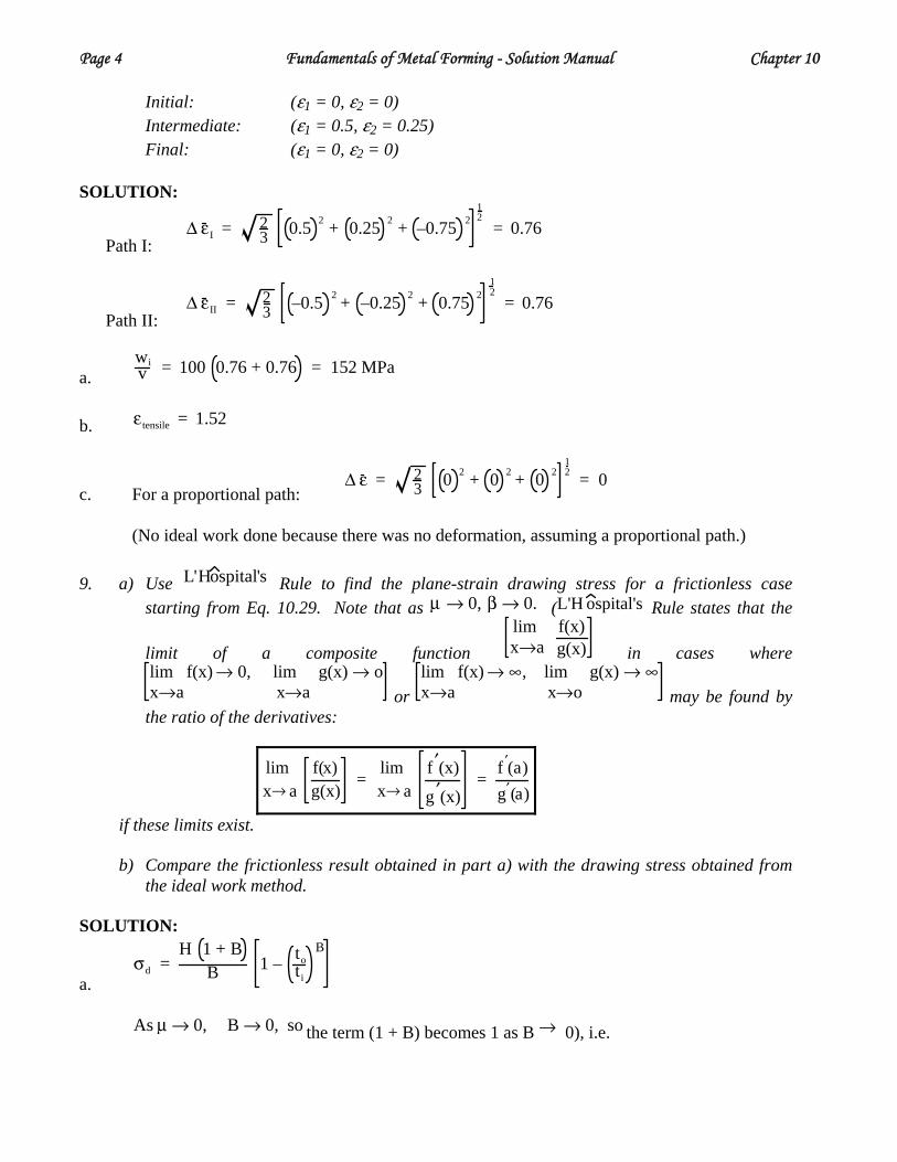
Page 4 Fundamentals of Metal Forming - Solution Manual Chapter 10
Initial: (ε1 = 0, ε2 = 0) Intermediate: (ε1 = 0.5, ε2 = 0.25) Final: (ε1 = 0, ε2 = 0)
SOLUTION:
Path I:
Δ εI = 2
3 0.5 2 + 0.25 2 + –0.75 212
= 0.76
Path II:
Δ εII = 2
3 –0.5 2 + –0.25 2 + 0.75 212
= 0.76
a. wi
v = 100 0.76 + 0.76 = 152 MPa
b. ε tensile = 1.52
c. For a proportional path:
Δ ε = 23 0 2 + 0 2 + 0 2
12 = 0
(No ideal work done because there was no deformation, assuming a proportional path.)
9. a) Use L'Hospital's Rule to find the plane-strain drawing stress for a frictionless case starting from Eq. 10.29. Note that as μ → 0, β → 0. (L'H ospital's Rule states that the
limit of a composite function lim x→a f(x)
g(x) in cases where lim f(x) → 0, lim g(x) → ox→a x→a or
lim f(x) → ∞, lim g(x) → ∞x→a x→o may be found by
the ratio of the derivatives:
limx→ a
f(x)g(x)
=limx→ a
f ′(x)
g ′(x)=
f ′(a)g′(a)
if these limits exist.
b) Compare the frictionless result obtained in part a) with the drawing stress obtained from the ideal work method.
SOLUTION:
a.
σd =
H 1 + BB 1 – to
ti
B
As μ → 0, B → 0, so the term (1 + B) becomes 1 as B → 0), i.e.

Chapter 10 Fundamentals of Metal Forming - Solution Manual Page 5
limμ→o
σd = Hlim
B→o
1 –toti
B
B
so:
f = H 1 –
t ot i
Bwhich goes to 0 as B → 0
g = B which goes to 0 as B → 0
f ′(0) = – H ln
toti
toti
B= H ln
t it o
, and g ′ = 1 Note:ddx
ax = ax ln a
∴
limμ→o
σd = H lntoti
b. The results are identical.
10. Following the procedure of Exercise 10.3, derive an expression of the wire-drawing stress for the
Coulomb friction case. Show all of your steps clearly. SOLUTION:
Everything is the same except the friction law, so τf is replaced by μP in Eq. 10.3-3:
0 = r d σ1 + 2 σ1 + μP cot α – P dr
The same substitution occurs in Eq. 10.3-6:
P = μP tan α – σ r , or P =
σ r
μ tan α – 1 We then can remove P from the equilibrium equation:
0 = r d σ1 + 2 σ1 + κ σ r dr where κ ≡ μ cot α – 1
μ tan α – 1 And we use Eq. 10.3-10 as before to remove σ r:
0 = r d σ1 + 2 σ1 + κ σ 1 – κ σ dr = r d σ1 + 2 1 + κ σ1 – κ σ dr, or
drr
=– dσ1
2 1 + κ σ1 – κ σ . Integration completes the solution for a material which does not strain-harden:

Page 6 Fundamentals of Metal Forming - Solution Manual Chapter 10
drr
r i
ro
=d σ1
2 1 + κ σ1 – κ σ0
σd
ln
rori
= –12 1 +κ
ln1 + κ σd – κ σ
κ σ , or σ =κ σ
1 + κ 1 –rori
– 2(1 + κ)
11. Following derivations in the text and in Problems 9 and 10, complete the following table:
Calculation Type Wire Draw σd
Round Extrusion
Pext
Sheet Draw σd
Sheet Extrusion Pext
Slab (general α, μ)
Slab (any μ, small α)
Slab (μ = o)
Ideal Work
SOLUTION:
Wire Draw, sd Round Extrusion,Pext Sheet Draw, sd Sheet Extrusion,Pext
κ σ
1 + κ1 –
ro
r i
–2(1+κ)
κ σ
1 + κ1 –
ro
r i
–2(1+κ)
H κ
1 + κ1 –
to
ti
–(κ+1)
H κ
1 + κ1 –
to
ti
–(κ+1) Slab
B+1
Bσ 1 –
ro
r i
2B
B+1
Bσ 1 –
ro
r i
2B
H 1+B
B1 –
to
ti
B
H 1+B
B1 –
to
ti
B
Slab
(small α)
2 σ lnro
r i
2 σ lnro
r i
HB lnto
ti
HB lnto
ti
Slab (μ = 0)
2 σ ln
ro
r i
2 σ lnro
r i
HB lnto
ti
HB lnto
ti
Ideal Work
Where: B = μ cot α
κ =
μ cot α + 1μ tan α – 1
H = 23
σ
12. For each forming operation in Problem 11, show how much the external stress or pressure
changes by using the small angle approximation.

Chapter 10 Fundamentals of Metal Forming - Solution Manual Page 7
α = 20°,
a. Use "typical values": rin, tin = 30mm, rout, tout,t = 20mm, α = 20o, μ = 0.25, b. Use "extreme values": rin, tin = 40mm, rout, tout,t = 20mm, α = 45o, μ = 0.5.
SOLUTION:
cot α = 0.69
κ =
μ cot α + 1μ tan α – 1
=1.69
–0.91= –1.86
μ β μ= 0.25, =a. Typical values:
Small α:
σd (wire) =
0.69 + 10.69
σ 1 –23
2 0.69
= 1.050 σ
Large α:
σd (wire) =
–1.861 – 1.86
σ 1 –23
–2 1–1.86
= 1.086 σ
Wire draw difference = 3.3%
Small α:
σd (sheet) =
0.69 + 10.69
H 1 –23
0.69
= 0.598 H
Large α:
σ (sheet) = –1.86
d 1 – 1.86 H 1 – 23
– 1–1.86= 0.637 H
Sheet draw difference = 6.1%
b. Extreme values: α = 45°, μ = 0.5, β = μ cot α = 0.5
κ =μ cot α + 1μ tan α – 1
=1.5–0.5
= –3
Small α:
σ (wire) =
0.5 + 1d 0.5 σ 1 – 1
22 0.5
= 1.50 σ
Large α:
σ (wire) = –3
d 1 – 3 σ 1 – 12
–2 1–3= 1.41 σ
Wire draw difference = 6.3%
Small α:
σ (sheet) =
0.5 + 1d 0.69 H 1 – 1
20.5
= 0.879 H
Large α:
σ (sheet) = –3
d 1 – 3 H 1 – 12
– 1–3= 1.125 H

Page 8 Fundamentals of Metal Forming - Solution Manual Chapter 10
22%
Sheet draw difference =
13. Perform a slab calculation for plane-strain compression of a Hollomon material (σ = 600 MPa ε )0.25 subject to Coulomb friction (μ = 0.3). Assuming an initial geometry of ho = 100mm and bo = 50mm, plot the friction hill at several values of h/ho (0.75, 0.5, 0.25) and find Pmax and Paverage as a function of h/ho.
SOLUTION:
P = 2σ
3exp 2μ
hb2 – x , μ = 0.3, ho = 100mm, bo = 50mm
h, b, σ are found as follows:
hho
0.75 0.5 0.25
h 75 50 25
b =h o b o
h 67 100 200
ε = ln hh h o
-0.29 -0.69 -1.39
ε = 2 εh3 0.33 0.80 1.61
σ = 600 ε–0.25
455 MPa
567 MPa
676 MPa

Chapter 10 Fundamentals of Metal Forming - Solution Manual Page 9
0
2000
4000
6000
8000
0 20 40 60 80 100
Problem 10-13Pr
essu
re (M
Pa)
Distance from Center (mm)
h=25mm
h=50 mm
h=75mm
Note: These solutions assume Coloumb frictionthroughout, which may exceed the interfacialshear strength of the material at the interface
and thus not be accurate.
14. Consider the forging operation shown below. If the die material can withstand a contact pressure
of 1500 MPa and the workpiece exhibits a constant effective stress of 500 MPa, what is the minimum height to which the billet can be forged. Assume two cases: a) μ = 0.25, b) sticking friction.
h0 = 30 mm
b0 =30mm
SOLUTION:
a. Coulomb friction, μ = 0.25: Pmax = 1500 MPa = 2 σ
3exp μb
h
Constant volume:
ho bo = h b, b =h o b o
h = 900mm2
h
1500 MPa =
2 500 MPa3
exp0.3 b o ho
h2

Page 10 Fundamentals of Metal Forming - Solution Manual Chapter 10
∴ hmin = 900mm2
31500 MPa500 MPa
– 2
12 = 16.8mm
b. Sticking friction, Pmax = 1500 MPa = 2 σ
31 + b
2h
∴ hmin = 900mm2
31500 MPa500 MPa
– 2
12 = 16.8mm
15. Consider the drawing of a sheet which reduces both of its dimensions in the cross sections. Set up and derive the differential equation which governs the drawing operation. Show all of
your work and leave the resulting equation in the form of the following variables: P2, P3, dA2, dA3, α, β, μ, t, and σ1
Considering the symmetry of the operation and assuming a von Mises material, find the
ratio of the stresses σ1/σ2/σ3.
60 mm
β
30 mm
dA3
side view
30 mmα
15 mm
dA2
top view P2 acts on dA2
P3 acts on dA3
START MIDDLE ENDend view
60 mm
15 mm
2t
t30 mm30 mm
SOLUTION:
Force balance in the longitudinal direction:
0 = d σ 1 2 t2 + 2 P2 μ cos α + sin α d A 2 + 2 P3 μ cos β + sin β d A 3
The strain ratios may be found from the geometry:
εh = ln t
30 εw = ln 2 t60 = ln t
30 ε l = –2 ln t30 , so
εh / εw / ε l = –1 / –1 / 2, (same as uniaxial tension)

Chapter 10 Fundamentals of Metal Forming - Solution Manual Page 11
Therefore, the stress state must be the one for uniaxial tension, or one which differs from that by a hydrostatic pressure (which does not affect plastic deformation of a von Mises material):
∴ σ1 / σ2 / σ3 = σ ± P / ± P / ± P
B. DEPTH PROBLEMS 16. Find the efficiency of a wire drawing operation, as estimated by a slab calculation, assuming the
following parameters: σ = 1000 MPa, α = 10o, rin = 50mm, rout = 40mm, μ = 0.25. SOLUTION:
Wire draw slab solution:
σd =
B + 1B
σ 1 –ro
r i
2B
where B = μ cot α (small α) = 0.25 cot 10° = 1.42
σd = 242
1.42 1000 MPa 1 – 45
2.84= 800 MPa
Ideal work calculation:
σd ideal =
Wi
Vol= σ d ε
o
ε
= 1000 MPa 2 ln54
= 446 MPa
Efficiency =
Wi
Wa=
σd ideal
σd slab=
446 MPa800 MPa
= 56%
17. For the conditions presented in Problem 16, what is the maximum rinrout that can be performed?
SOLUTION:
Maximum draw stress = 1000 MPa
1000 MPa =
2.421.42
1000 MPa 1 –ro
r i
2.84
ro
r i min
= 1 –1.422.42
12.84
= 0.73, orro
r i max
= 1.37
18. a. Repeat Exercise 10.2 for the most general assumption that the redundant work is a fixed fraction of the friction work:
α = wr
wf , 0 ≤ α ≤ 1.
b. Show that your general expression reduces to the standard expression (Eq. 10.13) when α = 0. c. Show that your expression reduces to the improved expression (Eq. 10.2-10) when α = 1.
d. Compute dido
*
for the cases in Table 10.2 using your general expression with α (i.e. all non-ideal work is redundant work.) What are the differences compared with standard expression for these cases?
→ ∞
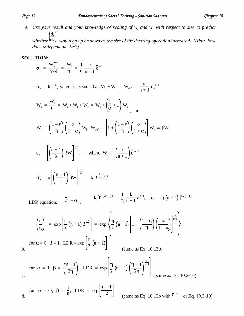
Page 12 Fundamentals of Metal Forming - Solution Manual Chapter 10
e. Use your result and your knowledge of scaling of wf and wr with respect to size to predict
whether dido
*
would go up or down as the size of the drawing operation increased. (Hint: how does α depend on size?)
SOLUTION:
a.
σd =
Watotal
Vol=
Wi
η =1η
kn + 1
εn+1
σa = k εa
n, where εa is such that Wi + Wr = Wdef =κ
n + 1εa
n+1
Wa =
Wi
η = Wi + Wf + Wr = Wi +1α + 1 Wr
, or
Wr =
1 – ηη
α1 + α
Wi, Wdef = 1 +1 – η
ηα
1 + αWi ≡ βWi
εa =
n + 1k
βWi
1n+1
, = where Wi =k
n + 1ε i
n+1
σa = κ
n + 1k
βWi
nn+1
= k βn
n+1 ε in
LDR equation: σa = σd , k βn (n+1)n (n+1) εn =
1η
kn + 1
εn+1, ε i = η n + 1 βn (n+1)n (n+1)
ro
r i
*
= expη2
n + 1 βn
n+1 = expη2
n + 1 1 +1 – η
ηα
1 + α
nn+1
b.
for α = 0, β = 1, LDR = exp
η2 n + 1
(same as Eq. 10.13b)
c.
for α = 1, β =η + 1
2η, LDR = exp
η2
n + 1η + 1
2η
nn+1
(same as Eq. 10.2-10)
d.
for α = ∞, β =
1η, LDR = exp
η + 12 (same as Eq. 10.13b with or Eq. 10.2-10) η = 1

Chapter 10 Fundamentals of Metal Forming - Solution Manual Page 13
Efficiency, material
η
n
d ido std.
*
(Eq. 10.13)
d ido improved
*
α = ∞
Difference
(%)
Ideal, brass 1.00 0.50 2.12 2.12 0%
Ideal, steel 1.00 0.25 1.87 1.87 0%
Medium, steel 0.70 0.25 1.55 1.87 21%
Low, steel 0.50 0.25 1.37 1.87 36%
Low, aluminum 0.50 0.15 1.33 1.78 34%
V. Low, zinc 0.25 0.00 1.15 1.65 43%
e. Imagine an operation with ri = 1 and draw length l = 1, and imagine scaling this operation by a factor C, i.e. ri = C, l = C. The deformation work will be proportional to the volume deformed, i.e. Wdef = (scale) = C3 Wdef. The friction work will depend on the swept surface, i.e. Wf = (scale) = C2 Wf. Therefore,
for α =
Wr
Wf→∞ as C → ∞ large operations and α → 0 as C → small operations .
Therefore, larger drawing operations can achieve somewhat larger draw ratios because friction plays a smaller role.
19. a) Derive equations similar to Eqs. 10.57 for the case of sticking friction. b) Assuming plane-strain conditions, eliminate P from your equations. c) By making appropriate geometric substitutions, write your equations in terms of t and dt
alone, and α and dα alone. SOLUTION:
a. For sticking friction, the friction stress is τ f = σ
3 whereas with Coulomb friction τf = μP . With this substitution, Eqs. 10.57a and b may be immediately rewritten:
0 = d σ 1 t + 2σ3
– 2P tan α d x1 before N (Neutral Point)
0 = d σ 1 t + – 2σ3
– 2P tan α d x1 after N (Neutral Point)
b. For plane-strain conditions (see Eq. 10.32), and small α:

Page 14 Fundamentals of Metal Forming - Solution Manual Chapter 10
P = σ1 +23
σ, so
0 = d σ t t + 2 ± σ
3σ1 – σ1 tan α – 2 σ
3tan α d x1
, where the plus sign is taken before the neutral point and the minus is taken after it.
c. Using the geometry shown, and defining a new variable t ′ as shown, the following geometric relationships may be obtained readily:
t ′ ≡ t – to
2 = R – R cos α
dt ′ = dt2 = R sin α dα
x1 = – 2 R t ′ – t ′2 = – R sin α
dx1 = –
R – t ′ dt ′
2 R t ′ – t ′ 2= – R cos α dα
t = 2 R – R cos α + to dt = 2R sin α dα
tan α = 2 R t ′ – t ′ 2
R – t ′ Then, in order to write the governing equation in terms of α and dα alone, we make the appropriate substitutions in the result of Part c:
0 = d σ t t + 2 ± σ
3– σ 1 tan α – 2 σ
3tan α dx1
d σ1 2 R – R cos α + to – R cos α dα
which, when rearranged, obtains:
0 = σ1 R sin α dα + 2 R – R cos α + to dσ1 – 2R ± σ
3cos α – σ1 sin α – 2 σ
3sin α dα
R
R
t'
R-t'
-x1
��������t/2
α
��������to/2
���ti/2
In order the write the same expression in terms of t and dt alone, we make a different set of substitutions:

Chapter 10 Fundamentals of Metal Forming - Solution Manual Page 15
0 = d σ t t + 2 ± σ
3– σ1 tan α – 2 σ
3tan α dx1
tan α = 2 R t ′ – t ′2
R – t ′ dx1 = –R – t ′ dt ′
2 R t ′ – t ′ 2
which, when rearranged, obtains:
0 = d σ 1 t + 2 +− σ
3R – t ′
2 R t ′ – t ′ 2+ σ 1 + 2 σ
3dt ′
where the minus sign applies before the neutral point and the plus sign afterward, and t' = t – to
2 and dt' = dt/2.
20. Real rolling operations exhibit several characteristics which are not easily seen in simple slab analysis. What do you think is the origin of the effects?
a) Plane sections do not remain planar
b)Internal cracking
c) Widening Side crackingd)
e) before
after
Crowning
SOLUTION: a. Friction at the rolls draws the sheet through the rolling operation, but since it operates only at the
surface, the central material tends to be restrained by the material behind it. b. The shear strains established by the gradient of friction force can cause shear banding, and strain
localization through the thickness. In fact, the tensile stress components along the rolling direction can also be large enough to produce cracking.
c. Widening occurs when the roll contact zone is comparable in the rolling direction relative to the

Page 16 Fundamentals of Metal Forming - Solution Manual Chapter 10
width of the contract region, so that the operation begins to resemble an upsetting operation. d. Side cracking can occur because shear strains are set up as the plane strain state in the center
approaches uniaxial compression at the edge. The tensile elongation caused by adjacent material can also introduce tensile stress cracking.
e. Crowning occurs by roll bending, i.e. the pressure across the roll causes beam-type bending of the rolls.
21. Consider a sheet-drawing operation (plane strain) that uses streamlined dies, as shown.
20mm30mm
a) Use a simple 5-step numerical procedure to find σ1 at t = 40mm, 36mm, 32mm, 28 mm, and 24 mm and 20mm.
b) What is the limiting tintout ratio that can be attained with these dies based on your numerical
procedure? How does this compare with the result for straight-sided dies? SOLUTION:
a. d σ1 = B σ1 – H 1 + B
dtt (Eq. 10.25)
Δ σ1 = B σ1 – H 1 + B
Δtt where H = 100 ksi and B = 0.25 cot [2 (t- 18)]
Step # t(mm) B Δt (mm) Δ σ1 KSi σ1 ksi
0 40 - - - - - - 0 (bdy. cond.)
1 36 0.34 -4 14.9 14.9 2 32 0.47 -4 17.5 32.4 3 28 0.69 -4 20.1 53.4 4 24 1.18 -4 25.9 79.3 5 20 3.58 -4 34.9 114.2
so, σd = 114.2 ksi. b. Interpolating between steps 4 and 5 to find the t where σd = 100 KS: yields
t* = 24 – 100 – 79.3
114.2 – 79.3 ⋅ 4mm = 21.6mm, or
ti
to
*
=40
21.6= 1.85
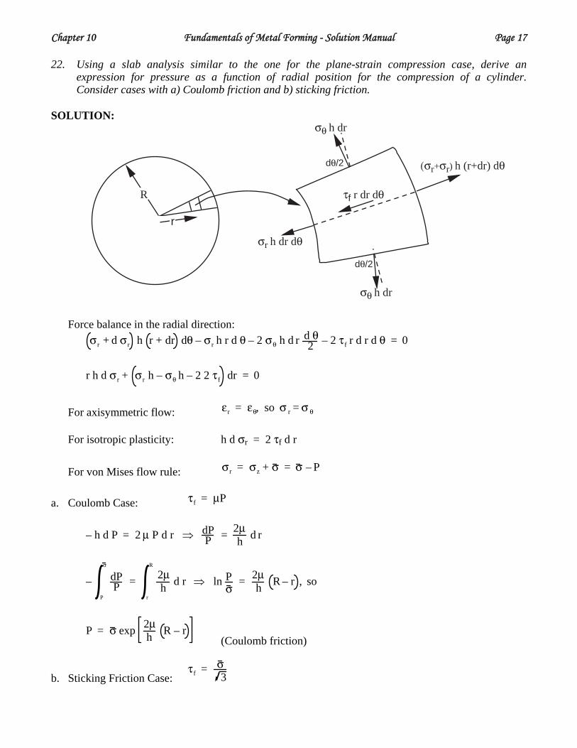
Chapter 10 Fundamentals of Metal Forming - Solution Manual Page 17 22. Using a slab analysis similar to the one for the plane-strain compression case, derive an
expression for pressure as a function of radial position for the compression of a cylinder. Consider cases with a) Coulomb friction and b) sticking friction.
SOLUTION:
R
r
dθ/2
dθ/2
σθ h dr
σθ h dr
(σr+σr) h (r+dr) dθ
τf r dr dθ
σr h dr dθ
Force balance in the radial direction:
σ r + d σr h r + dr dθ – σr h r d θ – 2 σθ h d r d θ
2 – 2 τf r d r d θ = 0
r h d σ r + σ r h – σθ h – 2 2 τ f dr = 0
For axisymmetric flow: εr = εθ, so σ r = σ θ
For isotropic plasticity: h d σr = 2 τf d r For von Mises flow rule: σr = σz + σ = σ – P
a. Coulomb Case: τf = μP
– h d P = 2 μ P d r ⇒ dP
P = 2μh d r
– dP
PP
σ
= 2μh d r
r
R
⇒ ln Pσ
= 2μh R – r , so
P = σ exp 2μh R – r
(Coulomb friction)
b. Sticking Friction Case: τ f = σ
3

Page 18 Fundamentals of Metal Forming - Solution Manual Chapter 10
– h d P = 2
3σ d r ⇒ dP = – 2
3 hσ d r
dP
P
σ
= 23
h σ d rr
R
P = σ +2σ3h
R – r (Sticking friction)
23. How would the sheet drawing stresses depend on normal plastic anisotropy (r) based on Hill's
theory? SOLUTION:
To find the effect of normal anisotropy, we need to substitute Hill's normal quadratic yield function (Eq. 7.60) in place of von Mises yield, and re-solve for σd. [Note, however that we conventionally choose σ3 normal to the sheet plane instead of x2 as was done previously for the sheet-draw problem.] For plane-strain (ε2 = 0) using Eq. 7.61b:
d ε2 = 0 = σ2 – σ3 – r σ1 – σ2
d ε1 + r σ
, so
σ2 =r
1 + rσ1 +
11 + r
σ3
Substituting into Eq. 7.60 (Hill's yield function):
σ =
2r + 11 + r
σ1 – σ3 (Hill) Which corresponds to the von Mises result (Eq. 10.22) for r = 1.
σ =
32
σ1 – σ3 (von Mises) Therefore, the replacement for Eq. 10.23 becomes
σ3 = σ1 – HHill, where HHill =1 + r2r + 1
σ
The final result corresponds to Eq. 10.29:
σd =
HHill 1 + BB
1 +to
ti
B
, where
HHill =1 + r2r + 1
σ
Therefore as r increases, σd increases.