chapter 1: introductory topics 1 - algebra 1.1 the real
TRANSCRIPT

Doyoung Park ECON 1078: Introductory Topics 1 - Algebra Lecture Note 1
Abstract
Page
1.1 The Real Numbers 1
1.2 Integer Powers 2
Properties of Powers . . . . . . . . . . . . . . . . . . . . . . . . . . . . . . . . . . . . . . . . . . . . 3
When do we use it in practice? . . . . . . . . . . . . . . . . . . . . . . . . . . . . . . . . . . . . . . 3
Chapter 1: Introductory Topics 1 - Algebra
1.1 The Real Numbers
The basic numbers you know of must be 1,2,3,... We call these numbers natural numbers. As you already
know, these numbers are comprised of even (2,4,6,...)and odd numbers (1,3,5,...). What if we include 0?
(i.e., 0,1,2,3,...) We refer these numbers as positive integers. It is possible to think of negative integers such
as -1, -2, ... and we generally name it as integers.
Rational numbers are those like 3/5 that can be written in the form of ab where a and b are both inte-
gers. Let’s think about 2. 2 can be express as 2/1, 4/2, 6/3, ... right? Thus, 2 is a rational number.
We learned that 2 is one of the natural numbers. So we can also learn that natural numbers are rational
numbers as well. Are all rational numbers are natural numbers then? The answer is NO. Let’s think of -2.
-2 is a rational number since it can be written as -2/1, -4/2, -6/3,... However, -2 is a negative integer, not a
natural number. Rational numbers can expressed using decimal system. We can easily calculate that 3/4 is
0.75. Rational numbers that use only a finite number of decimal places are called finite decimal fractions.
How about 100/3? It is obviously a rational number by definition and is equal to 33.333... We can see that
100/3 is using infinite decimal places. Hence we call this type of rational numbers as infinite decimal fractions.
Example. Changing circulation (recurring) decimals to rational number.
What makes it hard to change an infinite decimal fraction to a rational number is the circulation deci-
mals. So the key is to get rid of the recurring part. Let’s think about 33.333 · · · as an example and name it
as x. We multiply 10 to both hand side in order to erase recurring decimals by subtraction.
10x− x = 333.333 · · · − 33.333 · · · = 300 (1)
9x = 300⇔ x = 100/3 (2)
Practice Problem.
(1) 0.6767 · · ·
(2) 2.3454545 · · ·
Irrational numbers are numbers that cannot be written in the form of ab where a and b are both integers.√
2 is a good example.√
2 is 1.414213562... Therefore it is an infinite decimal fraction but not a rational
1.1 The Real Numbers continued on next page. . . Page 1 of 4

Doyoung Park ECON 1078: Introductory Topics 1 - Algebra Lecture Note 1
number since we cannot write it in the form of a/b. π is another typical example of irrational number. π is
3.141592654...
We call both rational and irrational numbers as real numbers and we will play with these numbers in
this semester.
Figure 1: Number System
Before we move to the next section, let me ask you brief question. Is 2/0 a rational number? How about
0/2? Also, is 0/0 a rational number?
1.2 Integer Powers
We have talked about number system in the previous section. Now, we will discuss about powers using real
numbers. Let’s think the following examples:
(1) 81
(2) 116
(3) − 127
What do all of these numbers have in common? These numbers can be expressed as products of real numbers.
(1) 81 = 9× 9 = 3× 3× 3× 3 = 34
(2) 116 = 1
4 ×14 = ( 1
4 )2 = 12 ×
12 ×
12 ×
12 = ( 1
2 )4
(3) − 127 = −( 1
3 ×13 ×
13 ) = −( 1
3 )3
From this example, we can derive a general rule of integer powers as follows:
an = a× a× ...× a︸ ︷︷ ︸n factors
where a is a real number and n is an integer. Now, let’s think about special cases.
(1) a is 0. → a numerical value is not assigned if n is 0.
(2) n is 0. → if a 6= 0, then an = 1.
(3) n is negative. (i.e., a−n where n is positive) → a−n = 1an where a 6= 0.
Example.
What is the difference between the two?
(1) (−10)2 vs. − 102
(2) (2x)−1 vs. 2x−1
1.2 Integer Powers continued on next page. . . Page 2 of 4

Doyoung Park ECON 1078: Introductory Topics 1 - Algebra Lecture Note 1
Properties of Powers
• an × am = an+m
• (an)m = anm
• an ÷ am = an−m = ana−m
• (ab)n = anbn
• (ab )n = an
bn = anb−n
? Be Careful!
• an × bn 6= (a+ b)n
• an ÷ bn 6= (a− b)n
• (a+ b)n 6= an + bn
Practice Problem.
(1) 36 × 34
(2) (52)6
(3) (4× 5)2
(4) ( 37 )4
(5) xpx2p
(6) ts ÷ ss−1
(7) a2b3a−1b5
(8) tptq−1
trts−1
(9) If x−2y3 = 5, compute x−4y6, x6y−9, and x2y−3 + 2x−10y15.
When do we use it in practice?
Compound Interest
Suppose you deposit $1000 in a bank account paying 8% interest at the end of each year. After 1 year
you will have earned $1000 · 0.08 = $80 in interest, so the amount in your bank account will be $1080. This
can be rewritten as
1000 + 1000 · 0.08 = 1000 · (1 + 0.08) = 1080
What would happen to your money in your bank account after 2 years?
1080 + 1080 · 0.08 = 1080 · (1 + 0.08) = 1000 · (1 + 0.08) · (1 + 0.08) = 1000 · (1.08)2
Suppose t is the time period, and $K is the amount of money you have initially deposited with p% interest
rate. Then we can derive the following general rule:
K · (1 +p
100)t
1.2 Integer Powers continued on next page. . . Page 3 of 4

Doyoung Park ECON 1078: Introductory Topics 1 - Algebra Lecture Note 1
Practice Problem.
A new car has been bought for $15,000 and is assumed to decrease in value (depreciate) by 15% per year.
What is its value after 6 years?
15000 · (1− 0.15)6 = 5657
Practice Problem.
How much money should you have deposited in a bank 5 years ago in order to have $1000 today, given
that the interest rate has been 8% per year over this period?
x · (1 + 0.08)5 = 1000
x =1000
(1 + 0.08)5
Suggested Problems.
p.8,9 Q.1 ∼ 6. Q.8 ∼ 10. Q.13
Page 4 of 4

Doyoung Park ECON 1078: Introductory Topics 1 - Algebra Lecture Note 2
Abstract
Page
1.3 Rules of Algebra 1
Algebraic Expressions . . . . . . . . . . . . . . . . . . . . . . . . . . . . . . . . . . . . . . . . . . . 2
Factoring . . . . . . . . . . . . . . . . . . . . . . . . . . . . . . . . . . . . . . . . . . . . . . . . . . 2
1.4 Fractions 3
Rules: . . . . . . . . . . . . . . . . . . . . . . . . . . . . . . . . . . . . . . . . . . . . . . . . . . . . 3
1.5 Fractional Powers 4
Properties of Square Root . . . . . . . . . . . . . . . . . . . . . . . . . . . . . . . . . . . . . . . . . 4
Nth Roots . . . . . . . . . . . . . . . . . . . . . . . . . . . . . . . . . . . . . . . . . . . . . . . . . . 4
Properties of Nth Root . . . . . . . . . . . . . . . . . . . . . . . . . . . . . . . . . . . . . . . . . . . 4
1.6 Inequalities 5
Implications - True or False? . . . . . . . . . . . . . . . . . . . . . . . . . . . . . . . . . . . . . . . 6
Comparing Two Real Numbers . . . . . . . . . . . . . . . . . . . . . . . . . . . . . . . . . . . . . . 6
Properties of Inequality . . . . . . . . . . . . . . . . . . . . . . . . . . . . . . . . . . . . . . . . . . 6
1.7 Intervals and Absolute Values 7
Absolute Value . . . . . . . . . . . . . . . . . . . . . . . . . . . . . . . . . . . . . . . . . . . . . . . 7
Chapter 1: Introductory Topics 1 - Algebra
1.3 Rules of Algebra
You are certainly familiar with the most common rules of algebra. Nevertheless, it may be useful to recall
those that are most important. If a,b, and c are arbitrary real numbers, then:
(a) a+ b = b+ a
(b) (a+ b) + c = a+ (b+ c)
(c) a+ 0 = a
(d) a+ (−a) = 0
(e) ab = ba
(f) (ab)c = a(bc)
(g) 1 · a = a
(h) aa−1 = a0 = 1 for a 6= 0
(i) (−a)b = a(−b) = −ab
(j) (−a)(−b) = ab
(k) a(b+ c) = ab+ ac
(l) (a+ b)c = ac+ bc
(m) (a+ b)(c+ d) = ac+ ad+ bc+ bd
Illustration of (m)
Figure 1: Sum of 4 areas
1.3 Rules of Algebra continued on next page. . . Page 1 of 8

Doyoung Park ECON 1078: Introductory Topics 1 - Algebra Lecture Note 2
Other Important Rules
(a) (a+ b)2 = a2 + b2 + 2ab
(b) (a− b)2 = a2 + b2 − 2ab
(c) (a+ b)(a− b) = a2 − b2
(d) (a+ b+ c)2 = a2 + b2 + c2 + 2ab+ 2bc+ 2ca
(e) (a+ b)3 = a3 + b3 + 3a2b+ 3ab2
Practice Problem.
(1) (3x+ 2y)2
(2) (1− 2z)2
(3) (4p+ 5q)(4p− 5q)
(4) (x+ 2y + 3c)2
(5) (3t+ 2s)3
(6) −(a+ b− c+ d)
Algebraic Expressions
Expressions involving letters such as 3xy − 5x2y3 + 2 are called algebraic expressions. Let’s try to expand
the following algebraic expressions:
(1) (2pq − 3p2)(p+ 2q)− (q2 − 2pq)(2p− q)
(2) (xy + 2yz)(1 + 2x) + (2 + 3y)(xy − 1)
Factoring
Factoring is a process to make the expanded algebraic expression back to a compact form. For example,
5x2y3 − 15xy2 = 5xy2(xy − 3).
Factoring Rule
Practice Problem.
(1) 5x2 + 15x
(2) −18b2 + 9ab
(3) K(1 + r) +K(1 + r)r
1.3 Rules of Algebra continued on next page. . . Page 2 of 8
Doyoung Park ECON 1078: Introductory Topics 1 - Algebra Lecture Note 2
(4) δL−3 + (1− δ)L−2
(5) 16a2 − 1
(6) x2y2 − 25z2
(7) 4u2 + 8u+ 4
(8) x2 − x+ 14
(9) 4x2 − y2 + 6x2 + 3xy
Suggested Problems.
p.13,14 Try to solve all problems.
1.4 Fractions
Recall that fraction can be expressed as
a÷ b =a
b
where a and b are called numerator and denominator respectively. If a is less than b (e.g., 5/8), then we call
this fraction a proper fraction. If the numerator is larger than the denominator, then it is called improper
fraction. An improper fraction can be re-written as a mixed number. (e.g., 19/8 = 2 + 3/8 = 238 )
Rules:
(a) a·cb·c = a
b (s.t b, c 6= 0)
(b) −a−b = (−a)·(−1)(−b)·(−1) = a
b
(c) −ab = (−1)a
b = (−1)ab = −a
b
(d) ac + b
c = a+bc
(e) ab + c
d = a·d+b·cb·d
(f) a+ bc = a·c+b
c
(g) a · bc = a·bc
(h) ab ·
cd = a·c
b·d
(i) ab ÷
cd = a
b ·dc = a·d
b·c
Practice Problem.
Simplify:
(1) 5x2yz3
25xy2z
(2) x2+xyx2−y2
(3) 4−4a+a2
a2−4
(4) 12 −
13 + 1
6
(5) 2+aa2b + 1−b
ab2 −2b
a2b2
(6) x−yx+y −
xx−y + 3xy
x2−y2
(7) 2+bab2 −
a−2a2b
(8) x−1x+1 −
1−xx−1 −
−1+4x2(x+1)
1.4 Fractions continued on next page. . . Page 3 of 8

Doyoung Park ECON 1078: Introductory Topics 1 - Algebra Lecture Note 2
Suggested Problems.
p.18,19 Try to solve all problems.
1.5 Fractional Powers
We will talk about the case where the power is a rational number: an where n is a rational number such as 12 .
If n = 1/2 then we have a12 . We define a
12 =
√a; square root of a where a ≥ 0. It would be mean-
ingful to recall the notion of square root.
We call x is a square root of a if x2 = a; x that satisfies the equation would be x = ±√a.
Do NOT forget that fact that a in the square root is greater or equal to 0; if it is nega-
tive then you have an imaginary number.
a1/2 =√a valid if a ≥ 0
Properties of Square Root
(a)√ab =
√a√b
(b)√
ab =
√a√b
(c)√a+ b 6=
√a+√b
Proof.
(a)√ab = (ab)1/2 = a1/2b1/2 =
√a√b
(b)√
ab = (a
b )1/2 = a1/2
b1/2=√a√b
Nth Roots
Now, we will talk about the situation where we have a power other than 1/2. Let’s first recall the definition
of square root.
x2 = a where a ≥ 0
We can generalize the above equation in the following way:
xn = a where a ≥ 0 and n is a natural number
Then the root (x) of this equation can be expressed as
x = n√a
and call x as the nth root of a.
Properties of Nth Root
(a) n√ab = n
√a n√b
(b) n√
ab =
n√a
n√b
1.5 Fractional Powers continued on next page. . . Page 4 of 8
Doyoung Park ECON 1078: Introductory Topics 1 - Algebra Lecture Note 2
(c) n√a m√a = a
1n+ 1
m
(d) anm = (a
1m )n = ( m
√a)n
Practice Problem 1.
Compute
(1) 3√
27
(2) ( 132 )1/5
(3) (0.0001)0.25
Practice Problem 2.
An amount $5,000 in an account has increased to $10,000 in 15 years. What yearly interest p% has been
used?
5000 · (1 +p
100)15 = 10000 or (1 +
p
100)15 = 2
(1 +p
100) = 2
115
(1 +p
100) = 2
115
∴ p = 100 · (2 115 − 1)
Practice Problem 3.
Compute:
(1) 1632
(2) 16−1.25
(3) ( 127 )−
23
(4) a3/8
a1/8
(5) (x1/2x3/2x−2/3)3/4
(6) ( 10p−1q2/3
80p2q−7/3 )−2/3
Suggested Problems.
p.22,23 Q.1 ∼ 5 Q.10 ∼ 12
1.6 Inequalities
The real numbers consist of the positive (+) numbers, 0, and the negative (-) numbers. If a is a positive
number, we write a > 0 (or 0 < a); a is greater than zero. What if we take the case where a is 0 into
account? Then, a ≥ 0; a is greater or equal to zero. If a is a negative number, we write a < 0 (or 0 > a); a
is less than 0. Of course we can also think the case that a is zero; a ≤ 0; a is less or equal to zero.
1.6 Inequalities continued on next page. . . Page 5 of 8

Doyoung Park ECON 1078: Introductory Topics 1 - Algebra Lecture Note 2
Implications - True or False?
(a) a > 0 and b > 0 imply a+ b > 0 and a · b > 0 (True)
(b) a+ b > 0 and a · b > 0 imply a > 0 and b > 0 (True)
(c) a > 0 or b > 0 imply a+ b > 0 and a · b > 0 (False)
(d) a+ b > 0 or a · b > 0 imply a > 0 and b > 0 (False)
Comparing Two Real Numbers
In general, we say that the number a is strictly greater than the number b, and we write a > b or b < a, if
a− b is positive:
a > b means that a− b > 0
If a > b or a = b, then we say that a is weakly greater than b and write it as
a ≥ b means that a− b ≥ 0
Properties of Inequality
(a) If a > b and b > c, then a > c
(b) If a > b and c > 0, then ac > bc ;
If the two sides of an inequality are multiplied by a positive number, then direction of the inequality
is preserved.
(c) If ac > bc and c > 0, then a > b
(d) If a > b and c < 0, then ac < bc ;
If the two sides of an inequality are multiplied by a negative number, then direction of the inequality
is reversed.
(e) If ac > bc and c < 0, then a < b
(f) If a > b and c > d, then a+ c > b+ d
Practice Problem 1.
Find what values of x satisfy 3x− 5 > x− 3
Practice Problem 2.
Find all values of x that satisfy (x− 1)(3− x) > 0
Practice Problem 3.
Find all values of p that satisfy 2p−3p−1 > 3− p.
Practice Problem 4. - Double Inequalities
Two inequalities that are valid simultaneously are often written as a double inequality.
(1) 3 < 2x ≤ 4
(2) 5 ≤ 3p+ 1 < 7
1.6 Inequalities continued on next page. . . Page 6 of 8

Doyoung Park ECON 1078: Introductory Topics 1 - Algebra Lecture Note 2
(3) One day, the lowest temperature in Buenos Aires was 50F , and the highest was 77F . What is the
corresponding temperature variation in degrees Celsius if F = 95C + 32?
50 ≤ 9
5C + 32 ≤ 77
(4) There are two axioms of probability: (a) the sum of probabilities is equal to 1, and (b) each probability
is bounded between 0 and 1. Using these axioms, what is the range of possible values of π?
X 1 2 3
P(X) 0.5− 2π −0.4 + 8π 0.9− 6π
Suggested Problems.
p.28,29 Q.1 ∼ 8
1.7 Intervals and Absolute Values
Let a and b be any two (real) numbers on the real line. Then we call the set of all numbers that lie between
a and b an interval. There are 4 types of intervals:
Notation Name The interval consists of all x satisfying:
(a, b) The open interval from a to b a < x < b
[a, b] The closed interval from a to b a ≤ x ≤ b(a, b] The half-open interval from a to b a < x ≤ b[a, b) The half-open interval from a to b a ≤ x < b
How do we denote the interval for “all numbers (weakly) greater than a? ( x > (≥) a). How about that of
all numbers (weakly) less than a? (x < (≤) a)
(a,∞) = all numbers x with x > a
[a,∞) = all numbers x with x ≥ a
(−∞, a) = all numbers x with x < a
(−∞, a] = all numbers x with x ≤ a
Absolute Value
The absolute value of a is denoted by |a|, and its definition is the following:
|a| =
a if a ≥ 0
−a if a < 0
Practice Problem 1.
(1) Compute |x− 2| for x = −3, x = 0, and x = 4.
(2) Rewrite |x− 2| using the definition of absolute value.
1.7 Intervals and Absolute Values continued on next page. . . Page 7 of 8

Doyoung Park ECON 1078: Introductory Topics 1 - Algebra Lecture Note 2
What is the implication of |x1 − x2|? This mathematical notation refers the distance between two
numbers on the number line.
Figure 2: Absolute value: distance between two points
If a is a positive number and |x| < a, then the distance from x to 0 is less than a. Furthermore, when a
is nonnegative, and |x| ≤ a, the distance between x and 0 is less than or equal to a. In symbols:
|x| < a means that− a < x < a
|x| ≤ a means that− a ≤ x ≤ a
Practice Problem 2.
(1) |3x− 2| ≤ 5
(2) |3− 8x| > 5
Suggested Problems.
p.31,32 Q.1 ∼ 3
p.32,33 Q.4 ∼ 5 Q.8, Q.11 ∼ 19
Page 8 of 8
Doyoung Park ECON 1078: Introductory Topics 2 - Equations Lecture Note 3
Abstract
Page
2.1 How to Solve Simple Equations 1
Rules to Solve a Simple Equation . . . . . . . . . . . . . . . . . . . . . . . . . . . . . . . . . . . . . 1
2.2 Equations with Two Variables and Parameters 2
2.3 Quadratic Equations 3
Quadratic Formula . . . . . . . . . . . . . . . . . . . . . . . . . . . . . . . . . . . . . . . . . . . . . 3
Discriminant . . . . . . . . . . . . . . . . . . . . . . . . . . . . . . . . . . . . . . . . . . . . . . . . 4
2.4 Linear Equations in Two Unknowns 4
2.5 Nonlinear Equations 4
Chapter 2: Introductory Topics 2 - Equations
2.1 How to Solve Simple Equations
In elementary mathematics, a variable is an alphabetic character representing a number, called the value of
the variable, which is either arbitrary or not fully specified or unknown. “Solving” an equation means that
we are trying to get the specific value (or all possible values) of the variable(s) that satisfies the equation.
We need to keep the following rules in mind in order to solve a simple equation.
Rules to Solve a Simple Equation
(a) Add or subtract the same number on both sides of equation
(b) Multiply or divide the same number (6= 0) on both sides of equation
We apply these rules to change the initial equation to the form of “x = ....” where only one hand side of
the equation has a variable. Let’s practice through the following problems.
Practice Problem.
Solve the equation.
(1) 6p− 12 (2p− 3) = 3(1− p)− 7
6 (p+ 2)
(2) x+2x−2 −
8x2−2x = 2
x
(3) zz−5 + 1
3 = −55−z
(4) A firm manufactures a commodity that costs $20 per unit to produce. In addition, the firm has fixed
costs of $2,000. Each unit is sold for $75. How many units must be sold if the firm is to meet a profit
target of $14,500?
profit = 14, 500 = TR− TC = PQ︸︷︷︸TR
− (FC + V C)︸ ︷︷ ︸TC
= 75Q− (2000 + 20Q)
2.1 How to Solve Simple Equations continued on next page. . . Page 1 of 5
Doyoung Park ECON 1078: Introductory Topics 2 - Equations Lecture Note 3
Suggested Problems.
p.36,37 Q1 ∼ 5.
2.2 Equations with Two Variables and Parameters
In the previous section, we have talked about the case where there is only one variable in the equation. Now,
we will think about equations that contains two variables. Suppose there is a positive linear relationship
between study hour and test score; the more I study, the higher score I get. Then we can express the
relationship of the two variable in the following way:
Test score = a+ b× Study hour where b > 0
Let the test score be y and study hour be x for simplicity. Then
y = a+ bx
As you can easily guess, we use equations with two (or multiple variables in general) variables in order to
describe a relationship between them. We know that x and y are called “variables” and these are the values
we are interested in.
a and b that specify the relationship between variables are called parameters. What is the difference
of variables and parameters? Variables are the values we want to know by solving equations; we call x and
y as “endogenous variables.” Parameters, however, are values that come from out of nowhere. Put it differ-
ently, these values are given exogenously and we do not ask questions how we got the values of parameters
or where its values are from.
Practice Problem.
Suppose the total demand for money in the economy is given by the formula
M = αY + β(r − γ)−δ
where M is the quantity of money in circulation, Y is national income, r is the interest rate, while α, β, γ,
and δ are positive parameters.
(1) Solve the equation for r.
(2) For the USA during the period 1929-1952, the parameters have been estimated as α = 0.14, β =
76.03, γ = 2, and δ = 0.84. Show that r is then given by
r = 2 + (76.03
M − 0.14Y)
2521
Suggested Problems.
p.40,41 Q.2 ∼ 5.
Page 2 of 5

Doyoung Park ECON 1078: Introductory Topics 2 - Equations Lecture Note 3
2.3 Quadratic Equations
This section reviews the method for solving quadratic (second-degree) equations. The general quadratic
equation has the form
ax2 + bx+ c = 0 (a 6= 0)
where a, b, andc are given constants, and x is the unknown variable. Again, our purpose is to figure out the
value of x using rules we have learned so far. Let’s think about the following examples.
Example.
(1) 5x2 − 8x = 0
(2) x2 − 4 = 0
(3) x2 + 3 = 0
(4) x2 + 8x− 9 = 0
Solution.
(1) 5x2 − 8x = x(5x− 8) = 0 Hence, x = 0 or x = 85
(2) x2−4 = 0⇔ x2 = 4 Hence, x = 2 or x = −2 or we can use factoring x2−4 = 0⇔ (x+2)(x−2) =
0 Hence, x = 2 or x = −2
(3) x2 + 3 = 0 since x2 is always positive, there is no solution (root) that satisfies this equation
(4) x2 + 8x− 9 = 0 ⇔ x2 + 8x− 9 = (x− 1)(x+ 9) = 0 Hence x = 1 or x = −9
Quadratic Formula
Quadratic formula directly gives us roots of an equation without applying factoring rule or rearranging all
terms to get a form of “x = ...”. We usually use this when factoring the equation is hard or even impossible.
If b2 − 4ac ≥ 0 and a 6= 0, then
ax2 + bx+ c = 0 if and only if x =−b±
√b2 − 4ac
2a
Let’s solve question (4) above using quadratic formula.
Since b2 − 4ac = 82 − 4(1)(−9) = 64 + 36 = 100 ≥ 0 and a = 1 6= 0 we can apply the formula.
x =−b±
√b2 − 4ac
2a=−8±
√82 − 4(1)(−9)
2(1)=−8±
√100
2=−8± 10
2=−18
2= −9 OR
2
2= 1
Practice Problem.
(1) 2x2 − 2x− 40 = 0
(2) 13x
2 + 23x−
143 = 0
(3) −2x2 + 40x− 600 = 0
2.3 Quadratic Equations continued on next page. . . Page 3 of 5
Doyoung Park ECON 1078: Introductory Topics 2 - Equations Lecture Note 3
Discriminant
b2 − 4ac is called discriminant and its sign tells us the number of solutions (roots) we have in the quadratic
equation.
(a) If b2 − 4ac > 0 then there are 2 roots.
(b) If b2 − 4ac = 0 then there is only 1 root.
(c) If b2 − 4ac < 0 then no root exist.
Suggested Problems.
p.44,45 Q.1 ∼ 4. Q.6
2.4 Linear Equations in Two Unknowns
In section 2.2, I have introduced the case where there are two variables in an equation and we know that this
equation describes the relationship between the two variables. The problem though is that it is impossible
to find out unique roots of such equation due to the fact that there is only 1 equation whereas we have two
unknown variables.
We have to keep in mind that the number of equations and that of unknown variables must coincide in or-
der to get unique solutions. In this section, we will learn how to get unique solutions in 2 by 2 framework;
2 variables and 2 equations.
2x+ 3y = 18 (1)
3x− 4y = −7 (2)
We need to find both x and y that satisfy two equations simultaneously. The first step is getting rid of
one variable; it can be either x or y - choose whatever you want to erase first. Suppose you want
to blow x away.
2x+ 3y = 6x+ 9y = 54 : multiply 3 on both hand side of equation (3)
3x− 4y = 6x− 8y = −14 : multiply 2 on both hand side of equation (4)
We can only have y on the left-hand side by subtracting eq.(3) and (4).
17y = 68⇔ y = 4 (5)
Next step is to get x by plugging y = 4 in one of the initial equations. Let’s plug 4 in eq. (1) for
example. Then we finally get x = 3.
Let’s get the roots by eliminating y this time. It is your tern to practice it!
Suggested Problems.
p.46,47 Q.1 ∼ 4.
2.5 Nonlinear Equations
We have thought about quadratic equations as the simplest examples of nonlinear equations. We can also
consider other general cases where equations are not linear as the following:
2.5 Nonlinear Equations continued on next page. . . Page 4 of 5
Doyoung Park ECON 1078: Introductory Topics 2 - Equations Lecture Note 3
(1) x3√x+ 2 = 0
(2) x(y + 3)(z2 + 1)√w − 3 = 0
(3) x2 − 3x3 = 0
Solution
(1) x3√x+ 2 = 0⇔ x3 = 0 or
√x+ 2 = 0⇔ ∴ x = 0 or x = −2
(2) x(y + 3)(z2 + 1)√w − 3 = 0 ⇔ x = 0 or y + 3 = 0 or z2 + 1 = 0 or
√w − 3 = 0 ⇔ ∴ x =
0 and/or y = −3 and/or w = 3
(3) x2 − 3x3 = 0⇔ x2(1− 3x) = 0⇔ x2 = 0 or 1− 3x = 0⇔ ∴ x = 0 or x = 13
Practice Problem 1.
What conclusions about the variables can we draw if
(1) x(x+ a) = x(2x+ b)
(2) λy = λz2
(3) xy2(1− y)− 2λ(y − 1) = 0
Practice Problem 2.
Solve the following equations (hint: check if the denominator can be 0):
(1) 1−K2√1+K2
= 0
(2) 45+6r−3r2
(r4+2)32
= 0
(3) x2−5x√x2−25 = 0
Suggested Problems.
p.49 Q.1 ∼ 3.
p.49,50 Q.1 ∼ 3. Q.5 ∼ 9.
Page 5 of 5

Doyoung Park ECON 1078: Introductory Topics 3 - Miscellaneous Lecture Note 4
Abstract
Page
3.1 Summation Notation 1
3.2 Rules of Summation and Newton’s Binomial Formula 2
Rules of Summation Operator . . . . . . . . . . . . . . . . . . . . . . . . . . . . . . . . . . . . . . . 2
Mean and Variance . . . . . . . . . . . . . . . . . . . . . . . . . . . . . . . . . . . . . . . . . . . . . 3
(Arithmetic) Mean . . . . . . . . . . . . . . . . . . . . . . . . . . . . . . . . . . . . . . . . . . 3
Variance . . . . . . . . . . . . . . . . . . . . . . . . . . . . . . . . . . . . . . . . . . . . . . . . 4
Newton’s Binomial Formula 5
3.3 Double Sums 5
3.4 A Few Aspects of Logic 6
Proposition . . . . . . . . . . . . . . . . . . . . . . . . . . . . . . . . . . . . . . . . . . . . . . . . . 6
Implication . . . . . . . . . . . . . . . . . . . . . . . . . . . . . . . . . . . . . . . . . . . . . . . . . 6
Necessary and Sufficient conditions . . . . . . . . . . . . . . . . . . . . . . . . . . . . . . . . . . . . 7
3.5 Mathematical Proofs - skip! 8
3.6 Essentials of Set Theory 8
Specifying a Property . . . . . . . . . . . . . . . . . . . . . . . . . . . . . . . . . . . . . . . . . . . 8
Set Membership . . . . . . . . . . . . . . . . . . . . . . . . . . . . . . . . . . . . . . . . . . . . . . 9
Set Operations . . . . . . . . . . . . . . . . . . . . . . . . . . . . . . . . . . . . . . . . . . . . . . . 9
Venn Diagrams . . . . . . . . . . . . . . . . . . . . . . . . . . . . . . . . . . . . . . . . . . . . . . . 10
3.7 Mathematical Induction - skip! 10
Chapter 3: Introductory Topics 3 - Miscellaneous
3.1 Summation Notation
Let’s suppose a country is divided into six regions, and we already know the population of each regions. If
we want to get the total population using the information we have, we need to use summation notation.
Let Ni be population of region i,
Total population = N1 +N2 +N3 +N4 +N5 +N6 =
6∑i=1
Ni
If there are n regions, then
N1 +N2 +N3 · · ·+Nn−1 +Nn =
n∑i=1
Ni ; sum of Ni from i = 1 to i = n
What if we want to get the population of 4 regions only? Let’s think about the total population from region
3 to 6 as an example.
N3 +N4 +N5 +N6 =
6∑i=3
3.1 Summation Notation continued on next page. . . Page 1 of 10
Doyoung Park ECON 1078: Introductory Topics 3 - Miscellaneous Lecture Note 4
Therefore, we can generalize the previous result as the following if we assume there are n regions in a country:
n∑i=p
Ni
We call i (it can be any alphabetical notation) summation index (or index of summation). When we
use summation notation, we must pay attention to this index since it indicates the terms that summation
notation is defined on.
Practice Problem 1.
Compute
(1)∑5i=1 i
2
(2)∑6k=3(5k − 3)
(3)∑2j=0
(−1)j(j+1)(j+3)
Practice Problem 2.
Expand
(1)∑ni=1 p
itqi
(2)∑1j=−3 x
5−jyj
(3)∑Ni=1(xij − xj)2
Suggested Problems.
p.54 Q.1 ∼ 3.
3.2 Rules of Summation and Newton’s Binomial Formula
Rules of Summation Operator
(a)∑ni=1 a = na ; a is a constant
(b)∑ni=1 aXi = a
∑ni=1Xi
(c)∑ni=1(a+ bXi) =
∑ni=1 a+
∑ni=1 bXi = na+ b
∑ni=1Xi
(d)∑ni=1(Xi + Yi) =
∑ni=1Xi +
∑ni=1 Yi
(e)∑ni=1(aXi + bYi + c) =
∑ni=1 aXi +
∑ni=1 bYi +
∑ni=1 c = a
∑ni=1Xi + b
∑ni=1 Yi + nc
Practice Problem 1.
Determine True/False of the following equations:
(1)∑
2Xi = 2∑Xi
(2)∑
2XiYi = 2∑XiYi
3.2 Rules of Summation and Newton’s Binomial Formula continued on next page. . . Page 2 of 10

Doyoung Park ECON 1078: Introductory Topics 3 - Miscellaneous Lecture Note 4
(3)∑
(Xi + Yi) =∑Xi +
∑Yi
(4)∑
(X2i + Y 2
i ) =∑X2i + Y 2
i
(5)∑
(2Xi + 3Yi) = 2∑Xi + 3
∑Yi
(6)∑
(2Xi + 3Yi + 4) = 2∑Xi + 3
∑Yi + 4
Mean and Variance
We use summation operator in Statistics to calculate the mean and variance. Let’s learn what these concepts
are.
(Arithmetic) Mean
We have 2 types of mean (or average): (a) population mean and (b) sample mean. Suppose we want to
know the GPA average of all students at CU. Let’s also assume that we are able to get the information of all
people. Then all students at CU is called population and we can calculate the GPA average in the following
way. Population mean of T CU students’ GPA is
µ =1
T
T∑i=1
Xi
Most of the case, however, it is very hard or even impossible to collect all data of our interest. Suppose we
choose 100 students at CU as a sample. Then the sample mean is
x =1
100
100∑i=1
Xi
In general,
x =1
n
n∑i=1
Xi ; n is a sample size
Practice Problem 2.
Let T be tax that varies by income level X and suppose total income in a geographical area containing 500
individuals is $5,000,000. What is the total tax revenue? What is the mean of income taxes? Tax is defined
as follows:
Ti = 0.1(Xi − 2000)
Solution500∑i=1
Ti =
500∑i=1
0.1(Xi − 2000) = ?
µ =1
500
500∑i=1
Ti =1
500
500∑i=1
0.1(Xi − 2000) = ?
3.2 Rules of Summation and Newton’s Binomial Formula continued on next page. . . Page 3 of 10
Doyoung Park ECON 1078: Introductory Topics 3 - Miscellaneous Lecture Note 4
Variance
We use variance to measure how much the data are dispersed from the mean. In other words, variance
implies the average distance between each datum and the mean. Then we can think of the following formula:
σ2 =1
T
T∑i=1
(Xi − µ)
There is a problem in this formula though.
1
T
T∑i=1
(Xi − µ) = 0
The given formula indicates that there is no dispersion of data from the mean although it actually exists.
This happens because negative distances (Xi < µ) offset positive distances (Xi > µ) on average. Therefore,
economists and statisticians use the modified formula that makes the distances all positive.
σ2 =1
T
T∑i=1
(Xi − µ)2 ; population variance
Applying the same logic, sample variance is
s2 =1
n
n∑i=1
(Xi − x)2
where n is the sample size.
Tips!
I know the formula of variance looks complicated. I want to introduce a simpler version of variance. Let’s
expand the formula and see what we get.
σ2 =1
T
T∑i=1
(Xi − µ)2 =1
T
T∑i=1
(X2i − 2µXi + µ2)
=1
T
T∑i=1
X2i − 2µ
1
T
T∑i=1
Xi +1
T
T∑i=1
µ2
=1
T
T∑i=1
X2i − 2µ
1
T
T∑i=1
Xi︸ ︷︷ ︸µ
+1
T
T∑i=1
µ2
︸ ︷︷ ︸µ2
=1
T
T∑i=1
X2i − µ2
= E(X2)− E(X)2
Practice Problem 3.
If X = 1, 2, 3, 4, 5, what is the mean and variance? Check if you get the same variance using E(X2)−E(X)2
formula.
3.2 Rules of Summation and Newton’s Binomial Formula continued on next page. . . Page 4 of 10
Doyoung Park ECON 1078: Introductory Topics 3 - Miscellaneous Lecture Note 4
Newton’s Binomial Formula
We already know that (a + b)1 = a + b and (a + b)2 = a2 + 2ab + b2. We have the formula that gives us a
generalized result (e.g., (a+ b)3, (a+ b)4 · · · etc.,).
(a+ b)m = amb0 +
(m
1
)am−1b1 +
(m
2
)am−2b2 + · · ·+
(m
m− 1
)a1bm−1 +
(m
m
)a0bm
Example.
(1) (a+ b)3 = a3b0 +(31
)a2b1 +
(32
)a1b2 +
(33
)a0b3
(2) (a+ b)4 = a4b0 +(41
)a3b1 +
(42
)a2b2 +
(43
)a1b3 +
(44
)a0b4
What is(nm
)?
We call it combination and it gives us the number of cases when we choose (pick) m goods (it can be
anything) out of n goods. For example, if you want to find out the total options to pick 2 marbles from 4
marbles, you apply combination. The answer is “4 combination 2” =(42
). Notice that we use combination
when the picking order does not matter.
How do we calculate combination?
Before we move on, let me introduce factorial. The notation of “k fatorial” is k! and defined as
k! = k × (k − 1)× (k − 2)× · · · × 3× 2× 1. For instance, 5! = 5× 4× 3× 2× 1.
Combination is defines as the following: (n
m
)=
n!
m!(n−m)!
Example.
(1)(42
)= 4!
2!2! = 6
(2)(53
)= 5!
3!2! = 5!2!3! =
(52
)= 10
From question (2), we can also derive an important property of combination.(n
m
)=
(n
n−m
)Suggested Problems.
p.59 Q.2, Q.3− (b)
3.3 Double Sums
What if we have multiple summation operators? How do we compute it? When you use summation operator
you should pay attention to summation index which indicates on which term that summation operator is
defined. Let’s think about the following example.
3.3 Double Sums continued on next page. . . Page 5 of 10
Doyoung Park ECON 1078: Introductory Topics 3 - Miscellaneous Lecture Note 4
3∑i=1
4∑j=1
(i+ 2j)
We can see two summation indices i and j. Summation operator indexed by i only affects the first term
i (i.e., i is regarded as a constant from j summation operator’s point of view) and the operator indexed by
j only influences on the second term j. Another important thing we should keep in mind is that we need to
think the double sum as “one operator” when we expand the given terms. Let’s compute the above example.
3∑i=1
4∑j=1
(i+ 2j) =
3∑i=1
4∑j=1
i+
3∑i=1
4∑j=1
2j
=
3∑i=1
4i+
4∑j=1
6j
= 4
3∑i=1
i+ 64∑j=1
j
= 4(1 + 2 + 3) + 6(1 + 2 + 3 + 4) = 24 + 60 = 84
Practice Problem 1.
Compute
(1)∑3i=1
∑4j=1 i · 3j
(2)∑mi=1
∑nj=1(i+ j2)
(3)∑3i=1
∑4j=1(2Xi + 3Yj)
(4)∑2i=1
∑5j=1(Xi + 3XiYj + 2Yj)
3.4 A Few Aspects of Logic
Proposition
This section deals with logical reasoning and the first thing I want to introduce you is proposition. A
proposition is an assertion that are either true or false. For example, “all people who breathe are alive” is a
true proposition while “all people who breathe are healthy” is a false proposition.
Implication
Now we will consider the relationship of two propositions P and Q. Suppose P and Q are two propositions
such that whenever P is true, then Q is necessarily true. In this case, we usually write
P =⇒ Q
The symbol ⇒ is an implication arrow and it addresses the direction of logical implication. We read
the above notation as
(i) “P implies Q”
(ii) “if P , then Q”
3.4 A Few Aspects of Logic continued on next page. . . Page 6 of 10
Doyoung Park ECON 1078: Introductory Topics 3 - Miscellaneous Lecture Note 4
(iii) “Q is the consequence of P”
(iv) “Q if P”
(v) “P only if Q”
(vi) “Q is an implication of P”
Example.
(1) x > 2 =⇒ x2 > 4
(2) xy = 0 =⇒ x = 0 or y = 0
(3) x is a square =⇒ x is a rectangle
(4) x is a healthy person =⇒ x breathes without difficulty
?? Contraposition ??
If P =⇒ Q then we have the contraposition ∼ Q =⇒∼ P . (∼ means “NOT”) Contrapositive proposition of
previous examples are
(1) x2 ≤ 4 =⇒ x ≤ 2
(2) x 6= 0 and y 6= 0 =⇒ xy 6= 0
(3) x is not a rectangle =⇒ x is not a square
(4) x breathes with difficulty =⇒ x is not a healthy person
We see that all contrapositions are true if the initial proposition is true. Hence, if you are confused
whether the given proposition is true or not, check the contraposition!
Equivalence
We can also easily see that this logical implication holds for all examples above. Let’s pay extra attention
on (2) since every propositions but (2) does NOT conversely hold.
We can express the logical equivalence of proposition P and Q by using equivalence arrow.
P ⇐⇒ Q
Necessary and Sufficient conditions
Suppose we have the following direction of logical implication regarding two propositions P and Q.
P =⇒ Q
Then we say that P is a sufficient condition for Q. At the same time, Q is called a necessary condition
for P . “P is a sufficient condition for Q” means that “if P holds, then Q automatically holds with no excep-
tions.” “Q is a necessary condition for P” addresses the fact that “although Q holds, P does not necessarily
(always) hold due to some exceptions.”
Let’s think about the previous examples again.
3.4 A Few Aspects of Logic continued on next page. . . Page 7 of 10
Doyoung Park ECON 1078: Introductory Topics 3 - Miscellaneous Lecture Note 4
(1) x > 2 =⇒ x2 > 4
(2) xy = 0 =⇒ x = 0 or y = 0
(3) x is a square =⇒ x is a rectangle
(4) x is a healthy person =⇒ x breathes without difficulty
Equivalence = necessary and sufficient = if and only if = iff
We know that (2) above is the case where the first and the second propositions are equivalent.
P ⇐⇒ Q
implies that P(Q) is a necessary and sufficient condition for Q(P) since “P is a necessary condition
for Q” means Q =⇒ P and “P is a sufficient condition for Q” means P =⇒ Q.
We also state the logical equivalence of two propositions using an expression if and only if or just simply
iff ; “P if (⇐=) and only if (=⇒) Q”
Suggested Problems.
p.65,66 Q.1 ∼ 7
3.5 Mathematical Proofs - skip!
3.6 Essentials of Set Theory
A set is a group of elements of the same kind. For example, we can make a set of fruits with apple, orange,
grape etc., as its elements. We denote a set with its elements as follows:
A = apple, orange, grape... where A is a set of fruits
Specifying a Property
Let’s imagine a case where we make two sets, A and B; one with odd and the other with even numbers.
Then we denote the two sets as
A = 1, 3, 5, 7, · · · where A is a set of odd numbers
B = 2, 4, 6, 8, · · · where B is a set of even numbers
We can also specify the property of a set instead of enumerating all elements.
A = y | y = 2x+ 1, x ≥ 0, x ∈ <
B = r | r = 2s, s ≥ 0, s ∈ <
How do we read this expression?
S = typical member | defining properties
The notation on the right hand side of | describes the condition (properties) that elements of a set satisfy.
The left hand side of | refers to the form of elements.
3.6 Essentials of Set Theory continued on next page. . . Page 8 of 10

Doyoung Park ECON 1078: Introductory Topics 3 - Miscellaneous Lecture Note 4
Set Membership
As briefly stated in the previous examples, there is a notation that denotes the relation between a set and
its members.
x ∈ S
means that x is an element of S.
To express the fact that x is NOT an element of S, we write
x /∈ S
For example, d /∈ a, b, c says that d is not an element of a, b, c.
We can also denote the relation between sets. Let A and B be any two sets. Then A is a subset of B
if every member of a set A is also a member of B.
A ⊂ B
If there is a chance that A is identical to B, then
A ⊆ B
Based on the same logic as before, if A is NOT a subset of B then
A 6⊂ B or A * B
What do the following two conditions imply?
A ⊆ B and A ⊇ B
Since A is a subset of B and at the same time B is a subset of A, it mean A = B.
Hence, we can express the equivalence of two proposition that
A = B iff A ⊆ B and A ⊇ B
Set Operations
As we have +,− in algebra, there are also operators in set theory as well.
Notation Name The set consists of:
A ∪B A union B x ∈ A or x ∈ BA ∩B A intersection B x ∈ A and x ∈ B
A−B or A \B A minus B x ∈ A and x /∈ BAc or A′ or A A complement x /∈ A
Additional Notations and Concepts
(i) Universal set (Ω): a set contains all arbitrary sets; family of sets.
(ii) Empty set (∅): a set which has no element.
3.6 Essentials of Set Theory continued on next page. . . Page 9 of 10

Doyoung Park ECON 1078: Introductory Topics 3 - Miscellaneous Lecture Note 4
(iii) Disjoint: if A ∩B = ∅ then A and B are disjoint.
Practice Problem 1.
Let A = 1, 2, 3, 4, 5 and B = 3.6. Find A ∪B, A ∩B, A−B, and B −A.
Venn Diagrams
Figures that illustrate the relations among sets are called Venn diagrams.
We can also plot three sets on the plane as well.
A ∩ (B ∪ C) = (A ∩B) ∪ (A ∩ C)
Practice Problem 2.
Plot the area using Venn-diagrams.
(1) (A ∩B) \ C
(2) (B ∩ C) \A
(3) (C ∩A) \B
(4) A \ (B ∪ C)
(5) B \ (C ∪A)
(6) C \ (A ∪B)
(7) A ∩B ∩ C
(8) (A ∪B ∪ C)c
Suggested Problems.
p.73,74 Q.1, 3, 5, 6
3.7 Mathematical Induction - skip!
Page 10 of 10

Doyoung Park ECON 1078: Functinos of One Variable Lecture Note 5
Abstract
Page
4.1 Introduction 1
4.2 Basic Definitions 2
Terminologies . . . . . . . . . . . . . . . . . . . . . . . . . . . . . . . . . . . . . . . . . . . . . . . . 2
Form of a function . . . . . . . . . . . . . . . . . . . . . . . . . . . . . . . . . . . . . . . . . . . . . 3
Functional Notation . . . . . . . . . . . . . . . . . . . . . . . . . . . . . . . . . . . . . . . . . . . . 3
4.3 Graphs of Functions 4
Some Important Graphs . . . . . . . . . . . . . . . . . . . . . . . . . . . . . . . . . . . . . . . . . . 6
4.4 Linear Functions 6
Terminologies . . . . . . . . . . . . . . . . . . . . . . . . . . . . . . . . . . . . . . . . . . . . . . . . 7
How Do We Compute The Slope? . . . . . . . . . . . . . . . . . . . . . . . . . . . . . . . . . . . . . 7
The Point-Slope and Point-Point Formulas . . . . . . . . . . . . . . . . . . . . . . . . . . . . . . . 8
Linear Inequalities . . . . . . . . . . . . . . . . . . . . . . . . . . . . . . . . . . . . . . . . . . . . . 9
4.5 Linear Models - skip 10
Chapter 4: Functions of One Variable
4.1 Introduction
Before we talk about functions, let’s first take a look at the following table. It shows personal consumption
level in accordance with time period. In other words, this table addresses the relation between the two
variable: consumption level and time.
The following figure shows how much tax revenue a government can collect depends upon the tax rate;
graph shows the relation between tax rate and government revenue.
4.1 Introduction continued on next page. . . Page 1 of 10

Doyoung Park ECON 1078: Functinos of One Variable Lecture Note 5
What do Table 1 and Figure 1 have in common? They both describes the relationship between two
variables of interest.
A function is a rule that addresses the relation between two (or multiple) variables; inputs and outputs.
4.2 Basic Definitions
A function of a real variable x with domain D is a rule that assigns a unique real number to each (every)
real number x in D. As x varies over the whole domain, the set of all possible resulting values f(x) is called
the range of f .
The definition of function contains some new concepts that we need to learn.
Terminologies
(a) Domain : A set of all inputs (e.g., year, tax rate)
(b) Codomain : A set of all possible outputs (e.g., personal consumption level, tax revenue)
(c) Range: A set of outputs from a function
(d) Unique: All inputs must be corresponding to a single output
Practice Problem 1.
Find a function (or functions) from the following correspondences.
4.2 Basic Definitions continued on next page. . . Page 2 of 10

Doyoung Park ECON 1078: Functinos of One Variable Lecture Note 5
Practice Problem 2.
Find the domains of (a) f(x) = 1x+3 , and (b) g(x) =
√2x + 4.
Let’s go back to our example above. The domain of a function that describes the relationship between
year and consumption level is 2003 - 2009. Also domain of a function illustrated in Figure 1 is the tax rate
from 0 to 100.
What is the codomain then? A set of all possible personal consumption level or tax revenue is called
codomain. The realized (resulting) values shown in the table and the figure is called range of a function.
Form of a function
We denote a function using an alphabet f . (you can use any notation you want such as g h etc) If f is a
function, y is usually used to refer the result of f at a certain point x; y is the output using x as an input.
Mathematical notation is
y = f(x)
We call x the independent variable, or the argument of f , whereas y is called the dependent vari-
able.
If a function is defined using an algebraic formula, the doman consists of all values of the
independent variable for which the formula gives a unique value.
In economics, x is often called the exogenous variable, which is supposed to be fixed outside the economic
model. y = f(x) determines the endogenous variable y that is driven from the model.
Functional Notation
We have numerous functional forms depends upon the (research) question we ask.
Example.
If you think the number of plants makes the air quality worse exponentially, we can think of any arbitrary
functional form like
y = f(x) = x2 or y = f(x) = x3 etc
where x is the number of plants. We need to have a good story why you assumed such functional form though.
4.2 Basic Definitions continued on next page. . . Page 3 of 10
Doyoung Park ECON 1078: Functinos of One Variable Lecture Note 5
Practice Problem 3.
The total dollar cost of producing x units of a product is given by
C(x) = 100x√x + 500
fro each nonnegative integer x. Find the cost of producing 16 units. Suppose the firm produces a units; find
the increase in the cost from producing one additional unit.
Suggested Problems.
p.85,86 Q.1 ∼ 6. , Q.8 ∼ 15.
4.3 Graphs of Functions
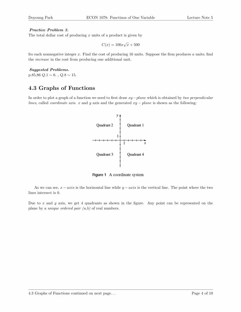
In order to plot a graph of a function we need to first draw xy−plane which is obtained by two perpendicular
lines, called coordinate axis. x and y axis and the generated xy − plane is shown as the following:
As we can see, x− axis is the horizontal line while y− axis is the vertical line. The point where the two
lines intersect is 0.
Due to x and y axis, we get 4 quadrants as shown in the figure. Any point can be represented on the
plane by a unique ordered pair (a,b) of real numbers.
4.3 Graphs of Functions continued on next page. . . Page 4 of 10

Doyoung Park ECON 1078: Functinos of One Variable Lecture Note 5
The graph of a function we will plot on xy − plane is the collection of all ordered pair (a,b) that satisfy
the function (rule). Thus remember that the specific form of ordered pairs are
(a, b) = (a, f(a)) for all a in the domain.
Note that ordered pair (a,b) is also called coordinates. For example, the coordinates of point P is (3,4).
Example 1.
Consider the function f(x) = x2 − 4x + 3. Make a table that shows the outcome where x = 0, 1, 2, 3, 4 and
plot the graph of this function.
Example 2.
Find some of the points on the graph of g(x) = 2x− 1, and sketch it.
4.3 Graphs of Functions continued on next page. . . Page 5 of 10

Doyoung Park ECON 1078: Functinos of One Variable Lecture Note 5
Some Important Graphs
There are more important forms graphs that we need to keep in mind.
Suggested Problems.
p.88,89 Q.1 ∼ 6
4.4 Linear Functions
Linear functions are assumed very often in economics for simplicity; demand and supply curves are regarded
as straight lines to simply calculate CS, PS and DWL. Linear functions take the form as follows.
y = ax + b where a and b are (real numbers) constants
As the title implies, the graph of the equation is a straight line and the function is called a linear function.
4.4 Linear Functions continued on next page. . . Page 6 of 10
Doyoung Park ECON 1078: Functinos of One Variable Lecture Note 5
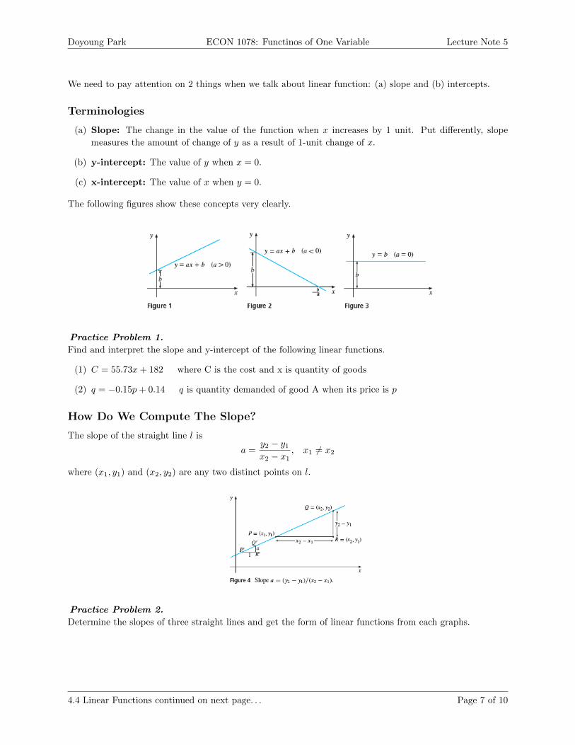
We need to pay attention on 2 things when we talk about linear function: (a) slope and (b) intercepts.
Terminologies
(a) Slope: The change in the value of the function when x increases by 1 unit. Put differently, slope
measures the amount of change of y as a result of 1-unit change of x.
(b) y-intercept: The value of y when x = 0.
(c) x-intercept: The value of x when y = 0.
The following figures show these concepts very clearly.
Practice Problem 1.
Find and interpret the slope and y-intercept of the following linear functions.
(1) C = 55.73x + 182 where C is the cost and x is quantity of goods
(2) q = −0.15p + 0.14 q is quantity demanded of good A when its price is p
How Do We Compute The Slope?
The slope of the straight line l is
a =y2 − y1x2 − x1
, x1 6= x2
where (x1, y1) and (x2, y2) are any two distinct points on l.
Practice Problem 2.
Determine the slopes of three straight lines and get the form of linear functions from each graphs.
4.4 Linear Functions continued on next page. . . Page 7 of 10

Doyoung Park ECON 1078: Functinos of One Variable Lecture Note 5
The Point-Slope and Point-Point Formulas
How do we get the functional form if
(a) only the slope a and a single point (x1, y1) are given?
(b) only two points (x1, y1) and (x2, y2) are given (i.e., no information about the slope)?
Case 1: Slope and a single point are known
We should keep in mind that the slope is given as a, and the slope between any arbitrary two coordi-
nates on the same line is the same.
If (x, y) is an arbitrary point on the same line with (x1, y1) which is given, then the slope of the line
passing (x, y) and (x1, y1) is
a =y − y1x− x1
From the above equation, we can derive the following form of linear function.
y = a(x− x1) + y1
Easier Way!
(1) Plug the given coordinate in the basic form of linear function: y1 = ax1 + b
(2) Get the y-intercept b by plugging given slope a into the equation you got in step 1.
Example 1.
Find a linear function that has slope −5 and passes (1, 2).
Step 1:
2 = a + b since y = ax + b is the basic form of linear function
Step 2:
2 = −5 + b→ b = 7
Therefore
y = −5x + 7
Case 2: Only two points are known
We know that two points (x1, y1) and (x2, y2) are on the same line. Hence we can calculate the slope.
4.4 Linear Functions continued on next page. . . Page 8 of 10

Doyoung Park ECON 1078: Functinos of One Variable Lecture Note 5
a =y2 − y1x2 − x1
Now we go back to case 1 where we know the slope and a point where the line passes through.
y =y2 − y1x2 − x1
(x− x1) + y1
y =y2 − y1x2 − x1
(x− x2) + y2
Easier Way!
(1) Get the slope a = y2−y1
x2−x1
(2) Get the y-intercept (b) by plugging any given coordinates y1 = y2−y1
x2−x1x1 + b
Example 2.
Find a linear function that passes (1, 2) and (4, 7).
Step 1: Get the slope.
a =7− 2
4− 1=
5
3
Step 2: Get the y-intercept
2 =5
3· 1 + b→ b =
1
3
Therefore
y =5
3x +
1
3
Linear Inequalities
What if a linear function is not binding?; we have inequality instead of equality.
Example 1.
Sketch in the xy-plane the set of all pairs of numbers (x, y) that satisfy the inequality 2x + y ≤ 4. (Using
set notation, this set is (x, y) | 2x + y ≤ 4)
Example 2.
Suppose a person consumes only two types of goods: good1 and good2. Price of each good is p1 and p2respectively. If the income of this person is m, sketch in the xy-plane the set of all possible pairs of con-
sumption bundle of good 1 and 2.
4.4 Linear Functions continued on next page. . . Page 9 of 10

Doyoung Park ECON 1078: Functinos of One Variable Lecture Note 5
We can write the budget set as
B = (x, y) | p1x1 + p2x2 ≤ m, x ≥ 0, y ≥ 0
Suggested Problems.
p.94,95 Q.1 ∼ 9
4.5 Linear Models - skip
Page 10 of 10

Doyoung Park ECON 1078: Functinos of One Variable Lecture Note 6
Abstract
Page
4.6 Quadratic Functions - Parabola 1
Shape and Position of Quadratic Functions . . . . . . . . . . . . . . . . . . . . . . . . . . . . . . . 1
Discriminant . . . . . . . . . . . . . . . . . . . . . . . . . . . . . . . . . . . . . . . . . . . . . . . . 1
Maximum and Minimum of the Parabola - Vertex . . . . . . . . . . . . . . . . . . . . . . . . . . . 2
Quadratic Opitmization Problems in Economics . . . . . . . . . . . . . . . . . . . . . . . . . . . . . 2
4.7 Polynomials 3
Polynomial Functions . . . . . . . . . . . . . . . . . . . . . . . . . . . . . . . . . . . . . . . . . . . 3
Polynomial Equation . . . . . . . . . . . . . . . . . . . . . . . . . . . . . . . . . . . . . . . . . . . . 4
Factoring Polynomials . . . . . . . . . . . . . . . . . . . . . . . . . . . . . . . . . . . . . . . . . . . 4
Polynomial Division with a Remainder . . . . . . . . . . . . . . . . . . . . . . . . . . . . . . . . . . 6
Chapter 4: Functions of One Variable
4.6 Quadratic Functions - Parabola
The form of quadratic function is
f(x) = ax2 + bx+ c where a, b and c are constants, a 6= 0
If a = 0, we go back to linear function; hence the restriction is a 6= 0)
Shape and Position of Quadratic Functions
In order to figure out the shape and the position of the parabola, there are 2 things we need to pay attention:
1) sign of a, and 2) sign of discriminant.
1) Sign of a is important!
When a > 0 the shape of the parabola looks like ∪, whereas if a < 0 the graph resembles ∩.
2) Sign of discriminant determines the position of the graph!
Let’s review what discriminant was.
Discriminant
b2 − 4ac is called discriminant and its sign tells us the number of solutions (roots) we have in the quadratic
equation: ax2 + bx+ c = 0
(a) If b2 − 4ac > 0 then there are 2 roots.
(b) If b2 − 4ac = 0 then there is only 1 root.
(c) If b2 − 4ac < 0 then no root exist.
If b2 − 4ac > 0, then the roots are
x =−b±
√b2 − 4ac
2a
4.6 Quadratic Functions - Parabola continued on next page. . . Page 1 of 6

Doyoung Park ECON 1078: Functinos of One Variable Lecture Note 6
We can get the roots by setting f(x) = y = 0 and apply the above rule. Hence, we see that these roots
are also called x− intercepts.
Let me rephrase the aforementioned properties of discriminant.
(a) If b2 − 4ac > 0 then there are 2 x-intercepts; the graph intersects with x-axis.
(b) If b2 − 4ac = 0 then there is only 1 x-intercept; the graph tangents to the x-axis.
(c) If b2 − 4ac < 0 then there is no x-intercepts; the graph neither intersects nor tangents to x-axis.
Therefore we have the following graphs of quadratic functions (parabola).
Maximum and Minimum of the Parabola - Vertex
We call the coordinates of the maximum or the minimum point P of the parabola vertex. How do we find
the vertex then?
We can factoring the quadratic function as follows.
f(x) = ax2 + bx+ c = a(x+b
2a)2 − b2 − 4ac
4a
What Do We Get?
(a) If a > 0, then f(x) = ax2 + bx+ c has its minimum at x = − b2a and the vertex is (− b
2a ,−b2−4ac
4a )
(b) If a < 0, then f(x) = ax2 + bx+ c has its maximum at x = − b2a and the vertex is (− b
2a ,−b2−4ac
4a )
Key Point!
We can get the max/min (depends on the sign of a) of the parabola by using the formula
x = − b
2a
and plugging this in the initial quadratic function to get the max/min value of y (i.e., f(− b2a )).
Quadratic Opitmization Problems in Economics
We will discuss how the rules we learned so far are applied in economics.
4.6 Quadratic Functions - Parabola continued on next page. . . Page 2 of 6

Doyoung Park ECON 1078: Functinos of One Variable Lecture Note 6
Practice Problem.
The price P per unit obtained by a firm in producing and selling Q units is P = 102− 2Q, and the cost of
producing and selling Q units is C = 2Q+ 12Q
2. Then the profit is
π(Q) = TR− TC = PQ− C = (102− 2Q)Q− (2Q+1
2Q2) = 100Q− 5
2Q2
Find the value of Q which maximizes profits, and the corresponding maximal profits.
We can easily notice that this quadratic function has a maximum since a = − 52 < 0. The rule we have
to remember was
x = − b
2a
Therefore,
Q = − 100
2 · (− 52 )
= 20
We can also get the corresponding maximized profits by plugging this value in the quadratic function.
π(20) = 100 · 20− 5
2· (20)2 = 1000
Suggested Problems.
p.103,104 Q.1 ∼ 6
4.7 Polynomials
Polynomial Functions
We have talked about linear and quadratic functions so far. We can derive cubic (polynomial of degree 3),
quartic (polynomial of degree 4) and other higher degree functions using the following form of polinomial
functions; the general polynomial function of degree n with coefficients a, b, c, d, · · · , e is
f(x) = axn + bxn−1 + cxn−2 + · · ·+ dx1 + e
If we assume a = 1, n = 3 with other coefficients to be zero; y = f(x) = x3, then the graph looks like the
red graph in the following figure.
The quartic function (degree 4), y = x4 looks like
4.7 Polynomials continued on next page. . . Page 3 of 6

Doyoung Park ECON 1078: Functinos of One Variable Lecture Note 6
Of course the shape of these graphs will be altered depends upon coefficients (in general, a quartic
function is a W shape curve). The following table summarizes forms and names of polynomial functions.
Question!
Are 5 + 1x2 and 1
x3−x+2 polynomials? Answer is No. If polynomials are in the denominator we don’t call the
whole term polynomials.
Polynomial Equation
If we set a polynomial function equal to 0 (to get x-intercepts (roots)) we get a polynomial equation.
f(x) = axn + βxn−1 + bxn−2 + · · ·+ cx1 + d = 0
This equation is called general equation of degree n. We use polynomial equation to find out the root(s).
A polynomial equation with degree n has at most n roots. Let’s think about a quadratic function. We
know that there are 3 possible cases where 1) the graph does not tangent x-axis, 2) touches x-axis and 3)
intersects with x-axis. This means that a quadratic equation can have 0, 1 or 2 roots.
Also it must be meaningful that a polynomial function with degree n has at most n − 1 “turning points.”
Recall that a quadratic function has 1 turning point.
Factoring Polynomials
Let P (x) and Q(x) be two polynomials for which the degree of P (x) is greater than or equal to the degree
of Q(x). Then there always exist unique polynomials q(x) and r(x) such that
P (x) = q(x)Q(x) + r(x) (Remainder Theorem)
where r(x) is called the remainder and its degree is less than that of Q(x). Put it differently,
4.7 Polynomials continued on next page. . . Page 4 of 6

Doyoung Park ECON 1078: Functinos of One Variable Lecture Note 6
P (x)
Q(x)= q(x) +
r(x)
Q(x)
This is not a new thing at all. Just recall how we do division using integers.
We know that 487 = 15 + 732 or just simply 487 = 15 7
32 . We can see that this rule applies to polynomials
as well.
What if r(x) = 0 and Q(x) is a polynomial of degree 1?
For example, P (x) = x3 − 3x2 − 50 and Q(x) = x− 5. Then
P (x) = x3 − 3x2 − 50 = q(x)Q(x) = (x2 + 2x+ 10)(x− 5)
In this case we say (x− 5) is the factor of polynomial P (x) = x3 − 3x2 − 50. Remember that this also
means 5 is a root of polynomial equation x3 − 3x2 − 50 = 0; P (5) = 0.
[Useful Fact! ]
Synthetic Division
Find the x-intercept first using the above tip! Start with that value!!
4.7 Polynomials continued on next page. . . Page 5 of 6

Doyoung Park ECON 1078: Functinos of One Variable Lecture Note 6
Practice Problem.
Prove that x− 5 is a factor of the polynomial P (x) = x3 − 3x2 − 50.
Practice Problem.
Find the root of polynomial equation P (x) = x3 − 3x2 − 50 = 0.
Practice Problem.
Find all possible integer roots of the equation 12x
3 − x2 + 12x− 1 = 0.
Practice Problem.
Find the root of polynomial equation P (x) = x4 + 2x3 − x− 30 = 0.
Practice Problem.
Polynomial Division with a Remainder
Perform the division: (x4 + 3x2 − 4)÷ (x2 + 2x)
Therefore
Suggested Problems.
p.111 Q.1 ∼ 5
Page 6 of 6

Doyoung Park ECON 1078: Functinos of One Variable Lecture Note 7
Abstract
Page
4.8 Power Functions 1
Graphs of Power Functions . . . . . . . . . . . . . . . . . . . . . . . . . . . . . . . . . . . . . . . . 1
4.9 Exponential Functions 3
The Natural Exponential Function . . . . . . . . . . . . . . . . . . . . . . . . . . . . . . . . . . . . 3
4.10 Logarithmic Functions 4
Relation between exponential and logarithmic function . . . . . . . . . . . . . . . . . . . . . . . . . 5
Logarithms with Bases other than e . . . . . . . . . . . . . . . . . . . . . . . . . . . . . . . . . . . 7
Chapter 4: Functions of One Variable
4.8 Power Functions
A power function f is defined by the formula
f(x) = Axr x > 0, r and A are any constants
Graphs of Power Functions
Let’s think the simplest version of power function: y = xr. Then there are 3 types of graphs that we can
think of.
What do all these figures have in common? Yes! All three graphs pass through the coordinate (1,1).
Why this happens? It is because y = 1 always when we plug x = 1 no matter what value of r we have.
A typical example of Figure 1 is y =√
2. The value of y does not increase as much as x does. That
is why we have a concave function.
If r = 3, for example, the value of y increases more rapidly than x does. Therefore we get a convex function.
What if the exponent is a negative real number? Let’s think y = x−1 = 1x If x > 1 then the value of
y decreases but incrementally slower speed as x increases constantly. If 0 < x < 1 then y decreases rapidly
than the amount of x increases. (or you can think y increases rapidly as the value of x decreases from 1 in
a constant manner.)
4.8 Power Functions continued on next page. . . Page 1 of 7

Doyoung Park ECON 1078: Functinos of One Variable Lecture Note 7
Figure 4 shows the graph of y = xr where values of r changes.
Practice Problem.
Solve the following equations:
(1) 22x = 8
(2) 33x+1 = 1/81
(3) 10x2−2x+2 = 100
Practice Problem.
Practice Problem.
Find t when
(1) 35t9t = 27
(2) 9t = (27)1/5/3
Page 2 of 7
Doyoung Park ECON 1078: Functinos of One Variable Lecture Note 7
4.9 Exponential Functions
Recall the form of a power function.
f(x) = Axr x > 0, r and A are any constants
We know that a power function has a variable x as the base of exponent r. Now, we will discuss a
functional form that has a variable as the exponent whereas the base is a constant.
Exponential function is defined as the following.
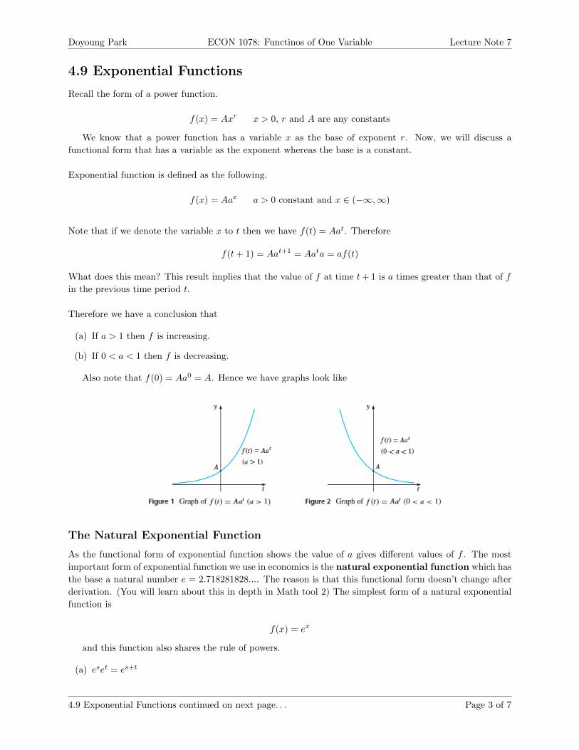
f(x) = Aax a > 0 constant and x ∈ (−∞,∞)
Note that if we denote the variable x to t then we have f(t) = Aat. Therefore
f(t+ 1) = Aat+1 = Aata = af(t)
What does this mean? This result implies that the value of f at time t+ 1 is a times greater than that of f
in the previous time period t.
Therefore we have a conclusion that
(a) If a > 1 then f is increasing.
(b) If 0 < a < 1 then f is decreasing.
Also note that f(0) = Aa0 = A. Hence we have graphs look like
The Natural Exponential Function
As the functional form of exponential function shows the value of a gives different values of f . The most
important form of exponential function we use in economics is the natural exponential function which has
the base a natural number e = 2.718281828.... The reason is that this functional form doesn’t change after
derivation. (You will learn about this in depth in Math tool 2) The simplest form of a natural exponential
function is
f(x) = ex
and this function also shares the rule of powers.
(a) eset = es+t
4.9 Exponential Functions continued on next page. . . Page 3 of 7
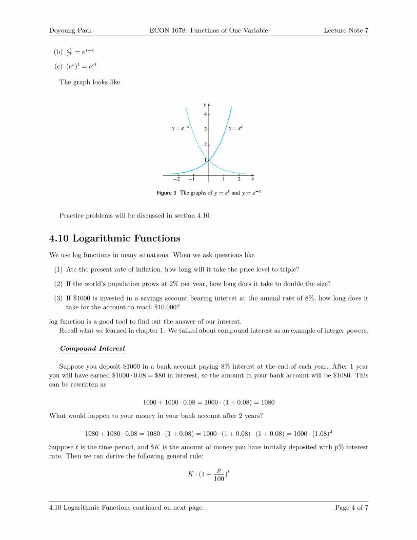
Doyoung Park ECON 1078: Functinos of One Variable Lecture Note 7
(b) es
et = es−t
(c) (es)t = est
The graph looks like
Practice problems will be discussed in section 4.10.
4.10 Logarithmic Functions
We use log functions in many situations. When we ask questions like
(1) Ate the present rate of inflation, how long will it take the price level to triple?
(2) If the world’s population grows at 2% per year, how long does it take to double the size?
(3) If $1000 is invested in a savings account bearing interest at the annual rate of 8%, how long does it
take for the account to reach $10,000?
log function is a good tool to find out the answer of our interest.
Recall what we learned in chapter 1. We talked about compound interest as an example of integer powers.
Compound Interest
Suppose you deposit $1000 in a bank account paying 8% interest at the end of each year. After 1 year
you will have earned $1000 · 0.08 = $80 in interest, so the amount in your bank account will be $1080. This
can be rewritten as
1000 + 1000 · 0.08 = 1000 · (1 + 0.08) = 1080
What would happen to your money in your bank account after 2 years?
1080 + 1080 · 0.08 = 1080 · (1 + 0.08) = 1000 · (1 + 0.08) · (1 + 0.08) = 1000 · (1.08)2
Suppose t is the time period, and $K is the amount of money you have initially deposited with p% interest
rate. Then we can derive the following general rule:
K · (1 +p
100)t
4.10 Logarithmic Functions continued on next page. . . Page 4 of 7

Doyoung Park ECON 1078: Functinos of One Variable Lecture Note 7
Practice Problem.
A new car has been bought for $15,000 and is assumed to decrease in value (depreciate) by 15% per year.
What is its value after 6 years?
15000 · (1− 0.15)6 = 5657
Practice Problem.
How much money should you have deposited in a bank 5 years ago in order to have $1000 today, given
that the interest rate has been 8% per year over this period?
x · (1 + 0.08)5 = 1000
x =1000
(1 + 0.08)5
We have learned how to get 1) the amount of money I will get after t years if I deposited $K with p%
annual interest and how to calculate 2) the volume I have to deposit to get targeted amount of money after
t years under p% annual interest.
What if we do NOT know the time period to get the targeted amount of money then?
Relation between exponential and logarithmic function
In order to understand a logarithmic function, we first need to think about its relationship with an exponential
function.
We can see that an exponential function and a logarithmic function are symmetric by y = x. Therefore
we start with simplest form of exponential function to understand out main topic logarithmic function.
y = ex
If we have an exponential function like above, we call x the natural logarithm of y, and denote x = lny.
Therefore we get the following result.
y = elny
This means lny must the power of e to get y.
4.10 Logarithmic Functions continued on next page. . . Page 5 of 7
Doyoung Park ECON 1078: Functinos of One Variable Lecture Note 7
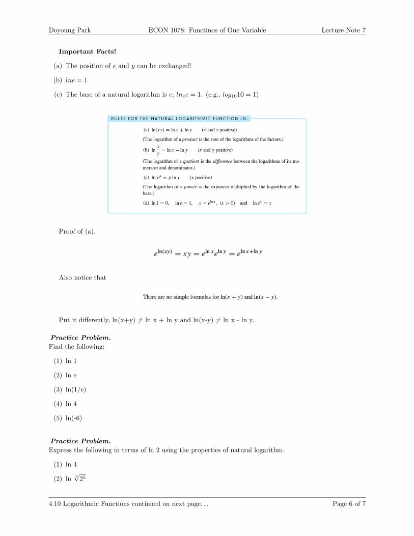
Important Facts!
(a) The position of e and y can be exchanged!
(b) lne = 1
(c) The base of a natural logarithm is e; lnee = 1. (e.g., log1010 = 1)
Proof of (a).
Also notice that
Put it differently, ln(x+y) 6= ln x + ln y and ln(x-y) 6= ln x - ln y.
Practice Problem.
Find the following:
(1) ln 1
(2) ln e
(3) ln(1/e)
(4) ln 4
(5) ln(-6)
Practice Problem.
Express the following in terms of ln 2 using the properties of natural logarithm.
(1) ln 4
(2) ln3√
25
4.10 Logarithmic Functions continued on next page. . . Page 6 of 7
Doyoung Park ECON 1078: Functinos of One Variable Lecture Note 7
(3) ln(1/16)
Practice Problem.
Solve the following equations for x:
(1) 5e−3x = 16
(2) Aαe−αx = k
(3) (1.08)x = 10
(4) ex + 4e−x = 4
Practice Problem.
Suppose you deposited $1000 in your bank account. How long does it take to get $15,000 if we assume the
annual interest rate is 8% and it doesn’t change?
Logarithms with Bases other than e
Logarithm with an arbitrary base a shares the same rule with ln :
Suggested Problems.
p.123, 124 Q.1 ∼ 3. Q.7
p.124, 125 Q.1, 3, 4, 5, 6, 7, 8, Q.14, 15, 16, 21
Page 7 of 7

Doyoung Park ECON 1078: Functinos of One Variable Lecture Note 8
Abstract
Page
5.1 Shifting Graphs 1
5.2 New Functions from Old 3
Products and Quotients . . . . . . . . . . . . . . . . . . . . . . . . . . . . . . . . . . . . . . . . . . 5
Composite Functions . . . . . . . . . . . . . . . . . . . . . . . . . . . . . . . . . . . . . . . . . . . . 5
Symmetry . . . . . . . . . . . . . . . . . . . . . . . . . . . . . . . . . . . . . . . . . . . . . . . . . . 5
5.3 Inverse Functions 6
A Geometric Characterization of Inverse Functions . . . . . . . . . . . . . . . . . . . . . . . . . . . 7
5.4 Graphs of Equations 8
Vertical-Line Test . . . . . . . . . . . . . . . . . . . . . . . . . . . . . . . . . . . . . . . . . . . . . . 9
Compound Functions . . . . . . . . . . . . . . . . . . . . . . . . . . . . . . . . . . . . . . . . . . . . 10
5.5 Distance in the Plane. Circles 11
Distance Between Two Points . . . . . . . . . . . . . . . . . . . . . . . . . . . . . . . . . . . . . . . 11
Distance Between Points on a Cirlce and the Center . . . . . . . . . . . . . . . . . . . . . . . . . . 12
5.6 General Functions - skip! 12
Chapter 5: Properties Of Functions
5.1 Shifting Graphs
This section studies in general how the graph of a function f(x) relates to the graphs of the functions
(1) f(x) + c
(2) f(x+ c)
(3) cf(x)
(4) f(−x)
Here c can be any positive or negative constant.
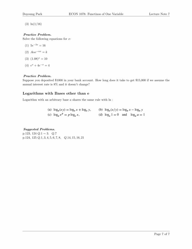
Example.
(1) y =√x
(2) y =√x+ 2
(3) y =√x− 2
(4) y =√x+ 2
(5) y =√x− 2
(6) y = 2√x
5.1 Shifting Graphs continued on next page. . . Page 1 of 12
Doyoung Park ECON 1078: Functinos of One Variable Lecture Note 8
(7) y = −√x
(8) y =√−x
We have general rules as follows. Memorizing these rules are important, but try to understand why these
rules hold. I recommend you to think
(a) How does the benchmark function look like?
(b) What are x and y intercepts?
5.1 Shifting Graphs continued on next page. . . Page 2 of 12

Doyoung Park ECON 1078: Functinos of One Variable Lecture Note 8
Practice Problem.
Sketch the graph of
(1) y = 2− (x+ 2)2
(2) y = 1x−2 + 3
(3) y = (x− 3)3 − 2
(4) y = −(x+ 2)3 + 1
(5) y = ln(x− 5) + 3
(6) y = −ln(x+ 3)− 1
(7) y = ex−3
(8) y = −ex−2 + 1
(9) y = |x|
(10) y = | − x|
(11) y = −|x|
(12) y = −|x+ 2|
(13) y = |x− 3|+ 2
Suggested Problem.
p.131, 132 Q.1, 2
5.2 New Functions from Old
This section discusses how to derive a new function from existing functions. For example, we can define
a function n(t) that refers the total number of students as the sum of two existing functions m(t) and
f(t) which indicate the number of male and female students at time t respectively: n(t) = m(t) + f(t) Or
if we are interested in differences of the numbers of male and female students, we can redefine n(t) as
n(t) = m(t)− f(t).
5.2 New Functions from Old continued on next page. . . Page 3 of 12

Doyoung Park ECON 1078: Functinos of One Variable Lecture Note 8
Example.
The cost of producing Q units of a commodity is C(Q). The cost per unit of output (average cost) is
defined as
A(Q) = C(Q)/Q
and suppose we know the cost function;
C(Q) = aQ3 + bQ2 + cQ+ d
Then the average cost function is
A(Q) =aQ3 + bQ2 + cQ+ d
Q= aQ2 + bQ+ c+
d
Q
We can see that A(Q) is the sum of two functions: 1) a quadratic function aQ2 + bQ+ c, and 2) a hyperboladQ .
Let’s suppose the market is perfectly competitive; P is given. Then we can also calculate profits of a
firm.
π(Q) = TR− TC = PQ− C(Q) = PQ− aQ3 + bQ2 + cQ+ d
5.2 New Functions from Old continued on next page. . . Page 4 of 12

Doyoung Park ECON 1078: Functinos of One Variable Lecture Note 8
Products and Quotients
We have talked about a new function which is driven by the sum or the difference of two (or multiple)
existing functions. We can also think about a function that is derived by multiplication or division of two
“old” functions.
We call h(x) is the product of f and g if
h(x) = f(x)g(x)
We call k(x) is the quotient of f and g if
k(x) =f(x)
g(x)
Composite Functions
In this section we will talk about the case where a function contains another function. We call y is a
composit functino of x if y is a function of u, and u is a function of x. We denote this situation using
mathematical notation
y = f(u) and u = g(x) → y = f(g(x)) or (f g)(x) or just simply f g
Note that
(f g)(x) = f(g(x)) whereas (g f)(x) = g(f(x))
When we calculate this composite function, we first focus on the interior function (kernel) g(x) and then
pay attention to the exterior function f(x) to g(x).
Practice Problem.
Write the following composite functions:
(1) y = (x3 + x2)50
(2) y = e−(x−µ)2 (µ is a constant)
Symmetry
Let’s recall what we learned in section 5.1.
(a) f(−x) means f(x) is reflected about y-axis.
(b) −f(x) means f(x) is reflected about x-axis.
Therefore we have the following results.
(a) If f(−x) = f(x) (the graph doesn’t change although it is reflected about y-axis) then we call f(x) an
even function. (e.g., y = x2)
(b) If f(−x) = −f(x) (the graph reflected about x-axis and y-axis are same) then we call f(x) an odd
function. (e.g., y = x3)
Suggested Problem.
p.136 Q.1, 2− (a), 2− (b), 3, 4
Page 5 of 12
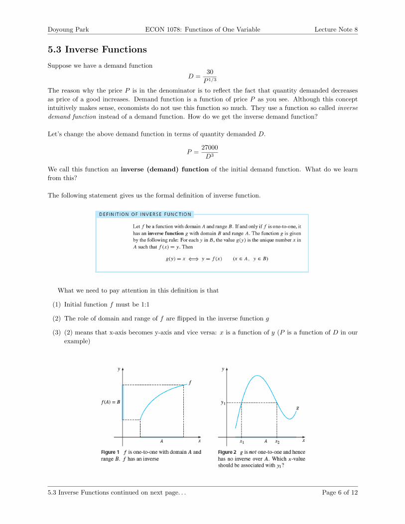
Doyoung Park ECON 1078: Functinos of One Variable Lecture Note 8
5.3 Inverse Functions
Suppose we have a demand function
D =30
P 1/3
The reason why the price P is in the denominator is to reflect the fact that quantity demanded decreases
as price of a good increases. Demand function is a function of price P as you see. Although this concept
intuitively makes sense, economists do not use this function so much. They use a function so called inverse
demand function instead of a demand function. How do we get the inverse demand function?
Let’s change the above demand function in terms of quantity demanded D.
P =27000
D3
We call this function an inverse (demand) function of the initial demand function. What do we learn
from this?
The following statement gives us the formal definition of inverse function.
What we need to pay attention in this definition is that
(1) Initial function f must be 1:1
(2) The role of domain and range of f are flipped in the inverse function g
(3) (2) means that x-axis becomes y-axis and vice versa: x is a function of y (P is a function of D in our
example)
5.3 Inverse Functions continued on next page. . . Page 6 of 12

Doyoung Park ECON 1078: Functinos of One Variable Lecture Note 8
Practice Problem.
Find the inverse functions of the following functions.
(1) y = 4x− 3
(2) y = 5√x+ 1
(3) y = 3x−1x+4
Note that the notation of an inverse function is to put −1 as the “exponent” of a function. If g is the
inverse function of f , it is denote g = f−1 or more formally g(y) = f−1(x). If a is an integer, then a−1 = 1a .
However, f−1 6= 1f(x) . For example, y = 1
x2+2x+3 and y = x2 + 2x+ 3 are not inverse to each other.
A Geometric Characterization of Inverse Functions
We saw that the inverse function of y = f(x) = 4x− 3 is x = g(y) = 14y + 3
4 . A function with respect to x
is expressed in terms of y; independent and dependent variable serve roles of each other. This means that
y-axis becomes a new x-axis and vice verse.
The problem is that we don’t like y-axis to be a horizontal axis and x-axis to be a vertical axis because
it is not the way we conventionally make the xy-plane. Then how do we express the inverse function keeping
our xy-plane untouched? Since x variable serves the function of y and y as x, we just write y instead of x
and x instead of y. Therefore the above inverse function can be expressed
y = f−1(x) =1
4x+
3
4
The fact that x and y serve each other’s role geographically means that the inverse function can be
derived by the reflection of the initial function about y = x axis. In other words, initial function and inverse
function are mirror images to each other.
In summary,
5.3 Inverse Functions continued on next page. . . Page 7 of 12
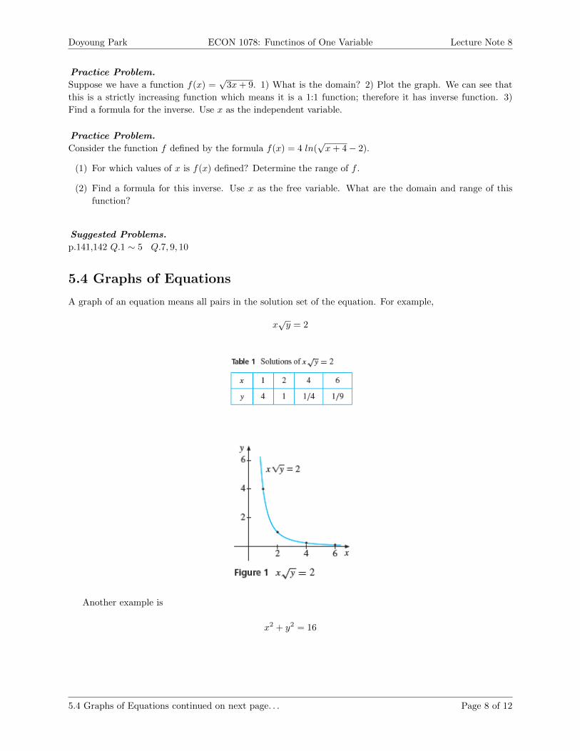
Doyoung Park ECON 1078: Functinos of One Variable Lecture Note 8
Practice Problem.
Suppose we have a function f(x) =√
3x+ 9. 1) What is the domain? 2) Plot the graph. We can see that
this is a strictly increasing function which means it is a 1:1 function; therefore it has inverse function. 3)
Find a formula for the inverse. Use x as the independent variable.
Practice Problem.
Consider the function f defined by the formula f(x) = 4 ln(√x+ 4− 2).
(1) For which values of x is f(x) defined? Determine the range of f .
(2) Find a formula for this inverse. Use x as the free variable. What are the domain and range of this
function?
Suggested Problems.
p.141,142 Q.1 ∼ 5 Q.7, 9, 10
5.4 Graphs of Equations
A graph of an equation means all pairs in the solution set of the equation. For example,
x√y = 2
Another example is
x2 + y2 = 16
5.4 Graphs of Equations continued on next page. . . Page 8 of 12

Doyoung Park ECON 1078: Functinos of One Variable Lecture Note 8
Vertical-Line Test
Plotting a graph on xy-plane does not necessarily mean that it is a graph of function. Put it differently, we
must differentiate graphs of equations and graphs of functions.
Do you remember the definition of function? A function assigns to each (every) point x in the domain
only one y-value; elements in domain cannot be matched with multiple elements in codomain.
This fact implies that the graph of a function has at most one point of intersection with a vertical line
through any point on the x-axis.
We plot a graph of x√y = 2 and x2 + y2 = 16. Which is a graph of function?
5.4 Graphs of Equations continued on next page. . . Page 9 of 12

Doyoung Park ECON 1078: Functinos of One Variable Lecture Note 8
Compound Functions
Sometimes a function is defined in several pieces, by giving a separate formula for each of a number of disjoint
parts of the domain.
Example.
Draw the graph of the function f defined by
Practice Problem.
Draw a graph of the following compound functions.
f(x) = 0 if x ≤ 0
= x2 if 0 ≤ x ≤ 1
= −(x− 1)2 + 1 if 1 ≤ x ≤ 2
= 0 if x ≥ 2
Practice Problem.
Page 10 of 12

Doyoung Park ECON 1078: Functinos of One Variable Lecture Note 8
5.5 Distance in the Plane. Circles
Distance Between Two Points
In this section, we will learn how to find the distance between two points.
Let P1 = (x1, y1) and P2 = (x2, y2) be two points in the xy-plane as shown in Figure 1.
As Figure 1 shows we can make a triangle with the base (x2 − x1) and the hight (y2 − y1).
Pythagoras’s Theorem
d2 = (x2 − x1)2 + (y2 − y1)2
By Pythagoas’s theorem, we have the following important formula to calculate the distance between two
distinct points:
Practice Problem.
Find the distance d between P1 = (−4, 3) and P2 = (5,−1).
Page 11 of 12

Doyoung Park ECON 1078: Functinos of One Variable Lecture Note 8
Distance Between Points on a Cirlce and the Center
What is the equation that represents a circle?
Equation of a Circle
x2 + y2 = r2
This is the most basic formula that describes a circle which is centered at (0, 0) with radius r. (Don’t forget
this b/c you can think of other size of circles from this equation.)
What is the equation that illustrates a circle centered at (a, b) with radius r?
Note that if x = a and y = b then the result of this equation is 0. This means that (a, b) is the center of
a circle because r represents the distance from the center to points on a circle.
Practice Problem.
Find the equation of the circle centered at (−4, 1) and radius 3.
Suggested Problems.
p.149 Q.1 ∼ 6
5.6 General Functions - skip!
Page 12 of 12