1

CHAPTER 1

INTRODUCTION

1.1 INTRODUCTION

Separation of blind sources, also called ‘waveform preserved blind

estimation of multiple independent sources’ is an emerging field of

fundamental research with many potential applications. It has garnered much

recent research and commercial interest in the fields such as digital and

wireless communications, signal processing, acoustics, medicine etc. Blind

Source Separation (BSS) is one of the fundamental and challenging problems

in Artificial Neural Networks (ANN) and Signal Processing fields. In many

practical situations, observations are modeled as linear/nonlinear mixtures of

a number of source signals, i.e., a Multi-Input Multi-Output (MIMO) system.

A typical example is speech recordings made in an acoustic environment in

the presence of background noise and/or competing speakers. Other examples

include Electrocardiograph (ECG) signals, passive sonar applications and

cross-talk in data communications (Hyvarinen and Oja 2000). The objective

of blind source separation is to separate unknown signals that have been

mixed together. The desired signals and the mixing matrix are not known and

the only available data being the mixture signal (Cruces et al 2004). There are

many possible applications of blind source separation. Some examples are

separation of radio signals for telecommunication, separation of signals

emanating from brain activity in medical applications and separation of

convolved speech signals including noise (Hyvarinen et al 2001).

2

The theories of BSS are applied to any kind of signals. This report

has focused on separation of birds voices and also speech signals. Hearing

aids, video conferencing etc., should disentangle one sound from other sounds

as human beings do. However, current techniques simply amplify the desired

signals and the competing noises without discrimination. This involves

multiple signals and multiple sensors and each sensor receives a mixture of

the source signals. When the transmission channels and original sources are

unknown, the BSS is a technique to retrieve these source signals from

observed mixture data.The cocktail-party problem is an example of BSS. This

is explained with an example. Suppose there is a conversation at a crowded

cocktail-party. It is usually a problem to focus on one person talking to

another person, since there is a wild mixture of different sounds originating

from various sources, like the conversation of many people in a room, the

stereo system playing background music etc. Despite all the background

noises, a system is programmed such that it separates the microphone

recordings into the different sound sources of the cocktail-party. Separating

out the speech of a person is the cocktail-party problem which is quite

difficult to solve, but it illustrates the goal of BSS i.e., it decomposes signals

that have been recorded by an array of sensors into the underlying sources.

1.2 BSS PROBLEM IN THE REAL WORLD

The BSS problem arises in diverse real time situations. For

example, a doctor records the ECG of a pregnant woman with several

electrodes located at her abdomen and her thorax in order to examine the heart

rhythm of the foetus. Besides other sources, the recorded signals contain the

heartbeat of the mother and also with much smaller amplitude, the heartbeat

of the foetus. The BSS problem in this situation is to separate the signal

generated by the foetus from the heartbeat of the mother. In another medical

context, neurologists monitor the electrical activity of the cortex with an

3

Electroencephalograph (EEG) in order to study the brain patterns evoked by

different stimuli. Current EEG systems record simultaneously upto hundreds

of electrodes. The obtained signals are a mixture of the activity of the

different areas in the brain, but also of artifacts such as the heartbeat or

movements of the eyeballs. The BSS problem is to remove the artifacts and to

decompose the EEG signals into signals originating from specific regions of

the brain. In a chemical plant, numerous sensors monitor the production

process. For quality control and much more importantly for early warning

systems, these sensor recordings are combined which leads to the BSS

problem of finding a clear representation of the recorded data by identifying

the relevant factors.

1.3 PRINCIPLE OF BSS

The most general BSS problem is formulated as follows. The block

diagram of mixing and non-mixing network is shown in Figure 1.1.

Figure 1.1 Block diagram of mixing and nonmixing network

BSS is a technique, which allows separating a number of source

signals from observed mixtures of those sources without a previous

4

knowledge of the mixing process (Lin et al 1997). Suppose there are ‘n’

observed signals, O1(t),O2(t),………..,On(t) for t = 1,2,……,T. These ‘n’

signals are modeled as linear combinations of ‘k’ unknown source signals

S1(t),S2(t),………,Sk(t) as given by

( ) ( )k

i ij jj 1

O t a S t for i 1,2,......,n=

= =∑ (1.1)

The coefficients aij determine what proportions of the sources Sj(t)

appear in the observed signal Oi(t). These coefficients form the mixing matrix

‘A’ which is assumed to be invertible and square. The recorded signals and

the source signals are viewed as multivariate time series as given by

( )

( )

( )

1

n

O t

.

O t .

.

O t

=

and ( )

( )

( )

1

k

S t

.

S t .

.

S t

=

(1.2)

The Independent component analysis model is sufficiently written as

( ) ( )tS.AtO = (1.3)

Because neither the mixing matrix ‘A’ nor the original sources S(t)

are known or observable, source separation is called a ‘blind’ technique. The

source signals S(t) are recovered by only analyzing the observed signals O(t).

However, the key is to assume that the source signals S1(t),S2(t),……..,Sk(t)

are statistically independent of each other. This is a quite plausible

assumption in the initial real world examples. For simplicity and without loss

of generality, the time step ‘t’ is omitted. The proposed algorithm determines

5

a separating matrix ‘W’ such that the resulting signals obtained as given in

Equation (1.4) are statistically as independent as possible.

M W.O= (1.4)

The ‘k’ components of ‘M’ are the original sources, called as

independent components. The three assumptions used to derive the objective

functions of most classical BSS algorithms from the maximum likelihood

principle in a uniform way are:

(i) At most one source has a Gaussian distribution.

(ii) The source signals have different spectra.

(iii) They have different variance profiles.

1.4 SIGNIFICANCE OF RADIAL BASIS FUNCTION NEURAL

NETWORK

In this section, the significances of Radial Basis Function (RBF)

neural network over other existing techniques are discussed. The BSS

algorithms, especially, Independent Component Analysis (ICA) and BSS

using temporal predictability (JTP) techniques are relatively simple

optimization procedures, but, they fail to find desirable signals if model or

some assumptions are not precisely satisfied. They can separate only linearly

mixed signals and they cannot recover the real scale of source signals. The

successful and efficient use of these techniques strongly depends on a priori

knowledge and selection of appropriate model. Moreover, these techniques

represent a set of random variables as linear functions of statistically

independent component variables. Therefore, according to basic ICA theory, a

solution to BSS problem exists and this solution is unique upto some trivial

indeterminacies (permutation and scaling) (Hyvarinen et al 2001). Even

6

though the nonlinear mixing model is more realistic and practical, most

existing blind separation algorithms developed so far are valid for linear

models. For nonlinear mixing models, many difficulties occur and both the

linear ICA theory and existing linear demixing algorithms are no longer

applicable because of the complexity of nonlinear characteristics. In addition,

there is no guarantee for the uniqueness of the solution of nonlinear blind

source separation unless some additional constraints are imposed on the

mixing transformation (Uncini and Piazza 2003).

RBF neural network is good at modeling nonlinear data and also

learn the given application quickly. It is a highly versatile and easily

implementable network. Since the instinct unsupervised learning of the RBF

neural network and blind signal processing are in essence unsupervised

learning procedures, the study of the RBF-based separation system seems

natural and reasonable. Further, an adaptive radial basis function neural

network developed in this work is different from those in the existing methods

and algorithms. By making use of the fast convergence and universal

approximation properties of RBF network, the new proposed demixing model

is proved to be better than the two existing algorithms with respect to the

performance index and the signal to noise ratio. In addition, the developed

unsupervised learning algorithm for RBF neural network appears naturally

suited and the structure of RBF networks is modular. The proposed RBF-

based system overcomes the limitations of the existing models such as highly

nonlinear weight update and slow convergence rate.

As given in Figure 1.2, the objective of the BSS problem is to find

an inverse neural system to estimate the original input signals. This estimation

is performed on the basis of only observed signal. Preferably, it is required

that the inverse system is constructed adaptively so that it has good tracking

capability under non-stationary environments. Then the appropriate energy

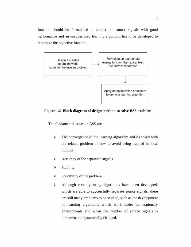
7

function should be formulated to extract the source signals with good

performance and an unsupervised learning algorithm has to be developed to

minimize the objective function.

Figure 1.2 Block diagram of design method to solve BSS problem

The fundamental issues in BSS are

� The convergence of the learning algorithm and its speed with

the related problem of how to avoid being trapped in local

minima

� Accuracy of the separated signals

� Stability

� Solvability of the problem

� Although recently many algorithms have been developed,

which are able to successfully separate source signals, there

are still many problems to be studied, such as the development

of learning algorithms which work under non-stationary

environments and when the number of source signals is

unknown and dynamically changed.

8

1.5 LITERATURE REVIEW

A brief review of the relevant literature on blind source separation

has been presented in this section. The review is intended to help in

developing a broad understanding of the different approaches that have been

employed in previous research for identification and extraction of

independent source signals. The neural network models with learning

capabilities for on-line blind separation of sources from linear mixture signals

have been first developed (Jutten and Herault 1986; Jutten et al 1991; Jutten

and Herault 1991). Jutten and Herault are the first to develop a neural

architecture and learning algorithm for blind source separation, since then a

number of variants on this architecture have appeared in the literature.

Comon (1994) gives the most complete analysis of the ICA

problem, justifying each of his steps in detail, as well as providing a

substantial literature review. He begins his development by pointing out the

inherent indeterminacy of ICA (due to scaling and permutation possibilities).

He makes a number of assumptions to make the problem theoretically

tractable. First, he assumes that the signals are noiseless. Second, he assumes

that only one component is Gaussian. Last he requires that ‘W’ is orthogonal.

Comon has showed at an earlier point in the paper that if at most one source

component is Gaussian, then pairwise independence is equivalent to mutual

independence. His algorithm boils down to looping through pairs of

components in the marginal density ‘z’ and rotating them in the plane in

which they exist (thus maintaining orthogonality of ‘Q’) such that the

orthogonality of ‘Q’ is maximized. He does not have theoretical bounds for

how many pairs need to be processed, but he finds empirically that 1 N+

sweeps (where sweep is an iteration through all unique pairs) are sufficient.

With this in mind, he empirically estimates the order of operations at O(N4).

9

One unfortunate aspect of the algorithm that adds significantly to

its computational complexity is that the marginal density ‘z’ is calculated

explicitly after each update of ‘W’ through ‘Q’. The author mentions that the

relationship between the cumulants of the observation ‘y’ and the cumulants

of ‘z’ would result in considerable savings per iteration, but this would

require computing the entire family of cumulants for ‘y’, which would

apparently outweigh the computational cost of the entire algorithm as it

stands.

Overall, the technique of Comon is well-motivated and seems to

perform well. It increases the contrast monotonically and completes in low-

order polynomial time. In empirical tests, he shows good convergence results,

even when the signal to noise ratio is quite low. However, there are a number

of places where his approach leaves something to be desired. First, while it

appears fairly efficient, it is a batch procedure and there are no obvious ways

to make it online since the latest ‘W’ has to be applied to all points before the

required cumulants can be estimated. In addition, although requiring the

demixing the matrix ‘W’ to be orthogonal greatly simplifies the math, it

greatly reduces the range of solutions as well, effectively removing one

degree of freedom. As a result, for example, two arbitrarily mixed signals

could not be separated using only two sensors, three would be necessary

unless they happened to be mixed with an orthogonal matrix. Therefore,

Comon's approach is a relatively slow batch method and is restricted in its

class of transforms, but it improves its contrast function monotonically with

each iteration and requires no knowledge of the source distributions (though

they must have non-null fourth-order cumulants).

Amari (1996), attempts to model the mutual information through a

series of approximations and then minimize it by different means. He also

normalizes the components to have zero mean and unit variance. He then

10

expands the marginal densities using the Gram-Charlier expansion. Amari

invokes the concept of the natural gradient. The limitation of this method is

that determining the structure of the parameter space can be difficult and can

lead to extremely complex algorithms. Even though this may be a more

effective gradient, there may still be the standard gradient descent problem of

choosing a step size. As far as it could be seen, there is no guarantee of

monotonic convergence using an arbitrary learning rate parameter.

Overall, the method of Amari has a number of advantages. His

method is online. It adapts one data point at a time by making real-time

implementations possible. His allowable class of transformations is the set of

non-singular matrices as opposed to Comon (1994) restriction to orthogonal

ones. However, there are some issues that remain to be resolved, particularly

in terms of convergence. While his argument for using the natural gradient is

appealing, its convergence properties in the case of BSS are not immediately

obvious. Therefore, Amari's method is mathematically appealing in that it

maximizes its contrast directly in the manifold of possible solutions, yet the

step size is an issue and there are no guarantees of smooth convergence,

especially considering the estimate of the cumulants by their instantaneous

values. Furthermore, the major empirical results are questionable in terms of

their convergence.

Murata and Ikeda (1998) have proposed an online algorithm for

convolutive mixture based on the notion of temporal structure of speech

signals. This online algorithm makes it possible to trace the changing

environment. The results are shown for a situation in which a person is

speaking in a room and moving around. They have used a Recurrent Neural

Network (RNN) for extracting independent components from the mixed

signals in each frequency channel. Strength of this proposed algorithm is that

it can follow the changing environment in time and separate the signals. But,

11

the limitations of their method are that the source signals are not completely

extracted when A(w) ≠ I + B(w,ts) (i.e., the mixing matrix is not equal to the

sum of the identity matrix and demixing matrix) and the different frequency

components from the same signal should be under the influence of a similar

modulation in amplitude.

The performances of the three neural algorithms (i) Fixed Point

(FP) ICA (ii) Joint Approximate Diagonalization of Eigenmatrices (JADE)

algorithm (iii) Extreme Event Analysis (eeA) are compared by Bedoya et al

(2003) for BSS in sensor array applications. The Fixed Point (or Fast) ICA

algorithm is based on Newton’s optimization method, which maximizes non-

gaussianity by means of minimizing negentropy, whereas Extreme Event

Analysis (eeA) algorithm is based on nonholonomic-nested Newton’s

methods, which minimizes the sum of squared fourth order cross cumulants

between components. The Fixed Point ICA algorithm is very fast in

convergence compared with other two algorithms. While the fixed-point

algorithm optimizes transform of the data, JADE algorithm optimizes the

transform of a particular set of statistics about the data.

The eeA algorithm is found to be slightly better than the other two

algorithms for large number of sources, since it determines the demixing

matrix with much cheaper computation. They have also showed that JADE

algorithm uses an eigenvalue decomposition of the 2 2N N× cumulant matrix

which replicates more separation time than the other two algorithms. The

accuracy of the separated signals is found to be more in JADE and FP using

Gaussian activation function than eeA algorithm and FP algorithm has less

computational load than the other two algorithms. The authors have also

showed that FP and JADE algorithms give better performance than eeA

algorithm for Gaussian noise sources. But their limitations are that they are

12

found to be poor performance, since they cannot find the directions of the

columns of the mixing matrix in order to locate the edges of the joint density

of the observations, when the maximization of the measure of nongaussianity

is done.

Li and Powers (2001) have analyzed the performance of speech

signal separation using Recurrent Neural Network (RNN) through fourth-

order statistics. They have introduced an unsupervised learning algorithm to

train RNN for speech signal separation. The drawbacks of this method are

that SNR for the separated speech signal 1 and speech signal 2 are 4.9dB and

6.7dB respectively, which are found to be very small and they produce

weights in undesirable local minima of the criterion function and higher order

statistics separates the signals only at the expense of heavy computational

complexity.

Uncini and Piazza (2003) have proposed a complex domain

adaptive spline neural network for blind signal processing. B-splines are used,

because they impose only simple constraints on the control parameters in

order to ensure a monotonously increasing characteristic. They have shown

experimental results on complex signals to show separation improvements

with respect to fixed activation functions. However, this method produces

only a fewer improvement for signal separation in frequency domain.

Adib et al (2004) have used reference signal as contrast function to

estimate the mixing matrix. The limitation of this method is that it can be used

only for classical instantaneous problems and there is a restriction that the

source signal cumulants of order ‘n’ under consideration exist with atmost

one cumulant zero. Zhu and Zhang (2002) have proposed a natural gradient

RLS algorithm for BSS. They have shown in simulations that their new

algorithm has faster convergence than the existing LMS and RLS algorithms

13

for BSS. But, its drawback is that its computational load is higher than the

existing algorithms. Cao et al (2003) have proposed prewhitening technique

and parameterized t-distribution technique to separate source signals which

contains mixtures of both sub-Guassian and super-Guassian noise. The merits

of the proposed method are that high level additive noise and its dimension

are reduced by the pre-whitening technique and the parameterized t-

distribution model separates the mixtures of sub-Guassian and super-Guassian

sources. The limitation of this method is that the co-variance of noise must be

known. But, it is usually unknown in the real world problems. So, this method

fails to separate the real-time source signals.

Fiori (2001) has derived a new learning algorithm as a nonlinear

complex extension of generalized Hebbian algorithm for a linear feedforward

network, called the Extended Hebbian learning Algorithm (EHA). He has

considered sequential and parallel version of EHA algorithm. To compare

these two versions, two parameters, the number of floating point operations

required for the algorithms to run, and the elapsed CPU times in seconds (on a

450 MHz, 64 MB machine), both averaged over the total number of extracted

components and over the total number of learning cycles for these two

approaches are analyzed. They have shown in experimental results that the

parallel version of EHA algorithm provides better performance than

sequential version. The limitations of these approaches are that the parallel

version is unable to converge properly with many sources and in the

sequential approach, extraction of errors is inevitably accumulated in each

step and its output quality is degraded progressively and it cannot be

employed in on-line operation.

Amari and Cichocki (1998) have presented few learning algorithms

and underlying basic mathematical ideas for the problem of adaptive blind

signal processing, especially, instantaneous blind separation and multichannel

14

blind deconvolution of independent source signals. They have discussed

recent developments of adaptive learning algorithms based on the natural

gradient approach and their properties concerning convergence, stability and

efficiency. The drawbacks of the natural gradient search method are that it is

required to invert the mixing matrix in each iteration in order to estimate the

source signals and some a priori knowledge about the mixing system and the

stochastic properties of the source signals must be known and the synaptic

weights should be generalized to real or complex valued dynamic filters

which results in increase in computational complexity.

Bell and Sejnowski (1995) take the approach of maximizing the output

entropy (which is related to minimizing mutual information and exactly

matches a maximum-likelihood criterion).They have developed an

information-maximization approach to blind signal separation. To find the

best demixing matrix, they simply maximize the output entropy, H(z) as their

contrast function. Maximization of the output entropy amounts to minimizing

the mutual information and thus finding the statistically most independent

components. This has obvious problems that there is no guarantee that the

global maximum of H(z) requires the minimization of mutual information

I(z); the increase in the marginal entropies could easily outweigh the

reduction in mutual information. In their experiments section, the authors

have shown that their algorithm can separate a combination of many signals

containing speech, music, laughter, etc. quite well using the logistic function

as the nonlinearity. However, there are simple cases where it fails. For

example, the increase in entropy for the wrong components outweighs the

increase in mutual information could be possible. Therefore, this method is

simple to implement and seems to work well empirically, but it is known to

have problems when there is a sufficient degree of mismatch between the

cumulative distribution function’s of the source distributions and the

components of the non-linearity.

15

Yang et al (1997) have used two-layer perceptron as a demixer and

both maximum entropy and minimum mutual information techniques to

derive their learning algorithms. This method extracts the signals from

observed nonlinear mixture signals, but one of the difficulties of using

minimum mutual information is the estimation of the marginal entropies. In

order to estimate the marginal entropy, the authors approximate the output

marginal probability density functions with truncated polynomial expansions

and a process that inherently introduces error in the estimation methods.

Hild et al (2001) have developed the Blind Source Separation using

Renyi’s Mutual Information. Unlike the Comon’s (1994) approach which uses

Shannon’s entropy and requires truncation of a probability density function

(pdf) series expansion, there are no approximations in the proposed method

due to utilization of Renyi’s quadratic entropy. Minimization of cost function

is performed by spatial whitening and rotation of the mixing matrix. The

strengths of this proposed model are that it requires only marginal entropy

estimation and avoids both polynomial expansions and estimation of Renyi’s

joint entropy. The limitation of this algorithm is that it is computationally

more complex since prewhitening and rotations are performed on the mixing

matrix.

In Joho et al (2001), the authors have used the natural gradient

method to extract the unknown source signals and interchannel interference is

used to measure the separation performance. The proposed method is able to

obtain faster convergence. But, its limitations are that it cannot separate the

sources without using the partial information of known signals and more

number of mixtures is needed to completely recover the original signals.

Bach and Jordan (2004) have presented an algorithm to perform

blind source separation of speech signals from a single microphone. To do so,

16

they have combined knowledge of physical and psychophysical properties of

speech with learning methods. The former has provided parameterized

affinity matrices for spectral clustering, and the later has used segmented

training data. The result is an optimized segmenter for spectrograms of speech

mixtures. However, this method is limited to the setting of ideal acoustics and

equal strength mixing of two speakers. First, the mixing conditions shall be

weakened and allow some form of delay or echo. Second, there are multiple

applications where speech has to be separated from a non-stationary noise.

Third, their framework is based on segmentation of the spectrogram and, as

such, distortions are inevitable since this is a ‘lossy’ formulation. Therefore,

some post-processing methods are needed to remove some of these

distortions.

The capabilities of Self-Organizing Maps (SOMs) in

parameterizing data manifolds to qualify them as candidates for blind

separation algorithms have been analyzed in Herrmann and Yang (1996). The

virtues and problems of the SOM-based approach in a simple example are

studied. Numerical simulations of more general cases have also been

performed. It has been shown that the performance is unquestionable in the

case of a linear mixture only if the observed data are pre-whitened and

inhomogeneities in the input data are compensated. This algorithm fails for

complex non-linearly distorted signals. Due to computational restrictions,

only mixtures from a few sources are resolved. SOM suffers from both

network complexity and interpolation errors for continuous phase signals.

SOM network is restricted only to a certain class of nonlinear functions in the

mixture.

Tan et al (2001) have proposed a Radial Basis Function neural network

for blind signal separation problems in the presence of cross nonlinearities. In

this paper, the contrast function that is the mutual information is chosen as

17

objective function, which measures the independence between various

sources. This function is minimized during training. The contrast function

used is based on the mutual information of the separating system outputs and

cumulant moment matching. They have added constraint on the output which

is the moment matching between the outputs of the separating system and

sources. They have developed two learning algorithms to separate the source

signals. In the first algorithm, all the parameters such as weight matrix,

centers of the Gaussian kernel and the radii of the activation function of RBF

neurons are updated and the mutual information is computed recursively. So,

this algorithm suffers from heavy computational burden. In the second

algorithm, they have adopted the self-organized learning algorithm which is

k-means clustering algorithm for selection of centres and radii of the hidden

neurons. The overall performance index, i.e. the moment matching is used as

the stopping criterion.

The proposed method improves the convergence rate and the

weight update is highly nonlinear. But, it suffers from the interpolation error

in recovering the original sources. The performance index of these algorithms

was found to be negative. Due to finite order moment matching i.e. upto 3rd

and 4th order, and local minima of the contrast function, the performance of

the network has to be still improved. Its performance degrades dramatically

when the source signals are characterized with frequent discontinuities.

Moreover, since the considerable level of performance is achieved at the cost

of large number of hidden nodes, it results in greater computational

complexity, stringent time requirements for training the network parameters

and less convergence of the blind RBF demixer, especially when the nodes

are not properly located in the input space. This also has a strong bearing on

how the parameters of the network are being initialized.

18

In Woo and Dlay (2005), RBF and BPN networks are cascaded.

The signals are recovered and reconstructed using a set of constraints. One of

the constraints is based on the property of Gaussian noise suppression in the

cumulant domain. In this network, minimizing contrast function takes more

computation time. This method updates the following.

• FMLP weights

• RBF weights

• Gradient Matrix M

• Threshold

• Width of RBF curve

Each update involves more complex computations. So, the overall

convergence speed of the demixer is extremely slow. To overcome these

expensive computations, the authors have updated the centre locations of the

neurons, which lead to less convergence speed. Considering the performance,

as shown in Figures 3 ‘e’ and ‘f’ in Woo and Dlay, the recovered signals still

have distortions compared with original source signals shown in their Figure

3(a). The performance index of this algorithm varies from 1.2 to 0.3 for SNR

varies from 5 to 25. Performance of the algorithm is reduced from 1.2 to 0.3

at the expense of higher computational intensity.

Lin and Lin (2006) have developed a RBF neural network

algorithm, which is compared with the Maximizing Entropy (ME) algorithm.

In this algorithm, the centre and width of the radial basis functions of hidden

neurons are updated and then weight vector is calculated by maximizing

entropy. They have used Φ(y) = y3 as the activation function and learning rate

parameter is kept at 0.0001. The performance of the algorithm is found by

using normalized cross-correlation. The performance index is found to be

between less than 0.35 and greater than 0 for iterations upto 8000. The

19

limitations of this algorithm are that it cannot separate the signals which are

nonlinearly mixed and it has been observed from their results that the

amplitudes of the recovered signals are less (-0.1 to 0.35) than that of the

original source signals (+1 to -1) and the recovered signals are also distorted

output.

Shoker et al (2005) have proposed both BSS and SVM to remove

the artifact signals such as heart rhythm and eye blinking from the statistically

independent sources. The merits of this proposed method is that not only it

separates the original sources but also it removes the artifact components

from the separated sources. But it has some limitations. It is necessary to

remix the independent sources and it fails to describe the generation of the

separated sources accurately due to the estimation errors in the sample

covariance matrices. Moreover, reprojection of extracted features results in

computational complexity.

Puntonet et al (2004) have proposed a theoretical method for

solving BSS-ICA using Support Vector Machine (SVM). Its objective

function is to minimize the Frobenius form of the unknown demixing matrix.

They have considered BSS problem as a convex optimization problem to

solve using SVM and it is solved using the Lagrange multiplier method

combined with an approximation to a given derivative of a convenient

discrepancy function based on cumulants. But, this method has more

limitations. It can separate only linearly mixed signals and range of possible

solutions to a problem is restricted. This method is not suitable if the

separation matrix does not exist as a linear function between independent

components and observed signals i.e., the convex optimization problem is not

feasible. This method is computationally quite expensive if the mixing matrix

is obtained by quadratic function or cubic function.

20

One of the statistical methods, ICA, uses higher order statistics in

an attempt to recover the independent components (Hyvarinen et al 2001).

The statistical tools and approximation techniques used in this method differ

significantly from the usual tools for the analysis of Gaussian random vectors,

and as a result have provoked interest in other areas, such as the machine

learning community. The major limitation of ICA is the inherent

indeterminacy due to scaling i.e., the real scale of source signals is not

recovered. When it is simulated and conducted experiments, it is observed

that it produces output with less scaling and the signal to noise ratio and

performance index of this algorithm is also found to be not satisfactory. Stone

(2001) has attempted another conventional algorithm for BSS using temporal

predictability which separates the original source signals by simultaneous

diagonalization of long and short term mixture covariance matrices. When its

simulation is run, it is noticed that it also produces output with less scaling

and the signal to noise ratio and performance index is not upto the reasonable

level.

Various statistical methods (Adib et al 2004; Xerri and Borloz

2004; Martinez and Bray 2003; Acernese et al 2003; Mukai et al 2006; Stone

2001; Pajunen 1998; Papadias and Paulraj 1997) and neural algorithms

(Amari et al 1996; Cichocki and Unbehauen 1996; Pajunen et al 1996; Meyer

et al 2006; Zhang et al 2004; Amari and Cichocki 1998; Fiori 2004; Zhang

et al 2001; Cruces et al 2004; Lindgren and Broman 1998) have been

developed by various researchers for blind signal separation. But only few

have been compared with other methods.

Having concluded that each of the above proposed methods has its

own strengths and weaknesses, the Artificial Neural Networks can be used to

solve BSS problem since they exhibit nonlinear input/output mapping

21

capabilities and can be trained with examples of a problem by

supervised/unsupervised algorithms to enable the network to acquire

knowledge about it. They can predict new outcomes from past trends and they

can learn by examples. Moreover, they are fault tolerant and robust and they

process information in parallel, at high speed and in a distributed manner. In

addition to these, Artificial Neural Networks are used where a conventional

process is not suitable; the conventional method cannot be easily delivered;

the conventional methods cannot fully capture the complexity in the data and

the stochastic behavior is important and an explanation of the network’s

decision is not required.

It is well known that neural network training can result in providing

weights in undesirable local minima of the criterion function. This problem is

particularly serious in recurrent neural networks as well as for multilayer

perceptrons with highly nonlinear activation functions because of their highly

nonlinear structure, and it gets worse as the network size increases. This

difficulty has motivated many researchers to search for a structure where the

output depends on the network weights is less nonlinear (Tan et al 2001). The

RBF network has a linear dependence on the output layer weights, and the

nonlinearity is introduced only by the cost function for training, which helps

to address the problem of local minima. The advantages of RBF network are

(i) Its training time is less.

(ii) It is good at modeling nonlinear data and also learns the given

application quickly. It is a highly versatile and easily

implementable network.

(iii) It finds the input to output mapping using local approximators.

Usually the unsupervised segment is simply linear combination

of approximators. Since linear combiners have few weights,

22

these networks train extremely fast and require few training

samples.

(iv) It provides faster convergence, smaller interpolation errors,

higher reliability and a more well-developed theoretical analysis

than BPN. (Haykin 2001)

.

The above characteristics of RBF neural networks motivate to develop an

Adaptive Self Normalized Radial Basis function neural network and an

unsupervised stochastic gradient descent algorithm for BSS problem. It is

noticed that a numerous attention has been aroused in solving BSS problems

in recent years with an increasing number of existing approaches. However,

much less attention has been received in comparison of performance of

various BSS algorithms. So, the proposed model is compared with two

existing ICA and JTP algorithms and it is proved that its performance is

improved over these two algorithms.

1.6 THESIS OBJECTIVES

The major objectives of the research work are

• To review the statistical technique Independent Component

Analysis (ICA) for blind source separation.

• To review the conventional method BSS using temporal

predictability (JTP) for blind source separation.

• To develop an Adaptive Self-Normalized Radial Basis

Function (ASN-RBF) neural network for blind source

separation.

23

• To develop an Unsupervised Stochastic Gradient Descent

learning Algorithm (USGDA) for separation of blind signals

and introduce a new parameter called convergence parameter

for the network to converge at a faster rate when the number

of sources is dynamically changed.

• To train the ASN-RBF neural network by USGDA algorithm

to extract independent source signals from a mixture signal,

with less training time than Backpropagation neural network

and eliminate the scaling problem of the two conventional

algorithms.

• To prove that the performance of the proposed algorithm is

improved over the ICA and JTP algorithms with respect to the

performance index and the signal to noise ratio.

1.7 THESIS ORGANIZATION

The thesis is organized into the following chapters.

Chapter 1: Introduction – This chapter provides a brief overview

of the blind source separation problem and presents the need for the study and

defines the problem. It reviews in detail the relevant literature on the problem

under study in general with particular emphasis on the earlier research and

approaches to extract the independent source signals from mixture signal. The

literature review is followed by the objectives of the research work and the

structure of the thesis.

Chapter 2: Statistical Models for blind source separation –This

chapter explains the two existing methods for blind source separation. It briefs

on advantages and drawbacks of these two methods.

24

Chapter 3: Artificial neural networks and learning algorithm –

This chapter presents the brief introduction about artificial neural networks

and learning algorithm. The ASN-RBF neural networks and unsupervised

learning algorithm developed and employed for extraction of independent

sources have been explained.

Chapter 4: Simulation results and discussion – It presents the

simulations carried out to test the ASN-RBF neural network and learning

algorithm.

Chapter 5: Comparison of performance measures of ICA, JTP

and USGDA algorithms – In this chapter, the performance of the proposed

algorithm has been compared with Independent Component Analysis and

BSS using Temporal Predictability algorithms with respect to the

performance index and the signal to noise ratio.

Chapter 6: Conclusion – This chapter summarizes the research

work. Certain conclusions have been made.