——————————————————–

CHAPTER 1

AN ELLIPSOIDAL PARTICLE-FINITE ELEMENT METHOD

FOR HYPERVELOCITY IMPACT SIMULATION

Ravishankar Shivarama1 and Eric P. Fahrenthold2

Department of Mechanical Engineering, 1 University Station C2200University of Texas, Austin, TX 78712, USA

1Graduate student2Professor, corresponding author, phone: (512) 471-3064, email: epfahren@mail.utexas.edu

https://ntrs.nasa.gov/search.jsp?R=20040191573 2020-05-12T14:57:22+00:00Z

AN ELLIPSOIDAL PARTICLE-FINITE ELEMENT METHOD

FOR HYPERVELOCITY IMPACT SIMULATION

Ravishankar Shivarama3 and Eric P. Fahrenthold4

Department of Mechanical Engineering, 1 University Station C2200University of Texas, Austin, TX 78712, USA

A number of coupled particle-element and hybrid particle-element methods have been de-

veloped for the simulation of hypervelocity impact problems, to avoid certain disadvantages

associated with the use of pure continuum based or pure particle based methods. To date

these methods have employed spherical particles. In recent work a hybrid formulation has

been extended to the ellipsoidal particle case. A model formulation approach based on La-

grange’s equations, with particles entropies serving as generalized coordinates, avoids the

angular momentum conservation problems which have been reported with ellipsoidal smooth

particle hydrodynamics models.

KEYWORDS: particle methods, finite element methods, impact simulation

INTRODUCTION

A review of the literature on hypervelocity impact simulation shows that most research in

this field has focused on the development and application of continuum hydrocodes, using ei-

ther Eulerian, Lagrangian, or Arbitrary Lagrangian-Eulerian (ALE) formulations [1,2,3]. In

the last decade attention has shifted towards particle based methods [4], in particular smooth

particle hydrodynamics (SPH). Although both continuum and particle based methods have

demonstrated excellent results in a range of practical applications, these methods are not

without problems. As a result some recent research has formulated coupled particle-element

3Graduate student4Professor, corresponding author, phone: (512) 471-3064, email: epfahren@mail.utexas.edu

2

[5] or hybrid particle-element [6] methods, aimed at avoiding certain disadvantages of the use

of pure continuum based methods or pure particle based methods in hypervelocity impact ap-

plications [7]. The present paper develops a generalized hybrid method, extending the work

of Fahrenthold and Horban [6], presenting for the first time a combined particle-element for-

mulation based on a nonspherical particle geometry. Nonspherical particle formulations are

also of interest in certain molecular dynamics [8] and astrophysics [9,10] applications, where

material or flowfield geometry has suggested the use of repulsion potentials or interpolation

kernels with ellipsoidal forms.

Most previous hypervelocity impact simulation work has employed Eulerian finite volume

and Lagrangian finite element methods [1,11] and more recent extensions of these methods

to Arbitrary Lagrangian-Eulerian frames [12]. Although continuum hydrocodes are accurate

and efficient simulation tools for many important problems, they are not well suited for use in

all hypervelocity impact applications. Eulerian codes can accommodate arbitrarily general

contact-impact, but their approximate models of material strength effects are best suited to

a very high velocity impact regime. Lagrangian codes incorporate very accurate models of

material strength effects, but their slideline based contact-impact algorithms are best suited

to a relatively low velocity impact regime. ALE methods allow for intelligent tailoring of the

mesh, ideally avoiding (but not eliminating) the preceding limitations.

None of the aforementioned continuum formulations is ideally suited to applications where

the generation, transport, and contact-impact dynamics of material fragments is of central

concern. When material fragments become much smaller than the finite volume cell size,

Eulerian flow field interpolations may not accurately represent the physical state of the highly

comminuted medium. Hence the adaptive introduction of a high resolution Eulerian mesh

is required. Similarly the use of Lagrangian finite elements to represent a highly fragmented

medium calls for the introduction of a very extensive and adaptive slideline mesh. It is

not surprising that these continuum formulations can be difficult to apply in cases where

fragmentation dynamics are of central interest, given the highly discontinuous nature of the

3

field variables in such systems.

Recognizing the disadvantages of continuum formulations in certain hypervelocity im-

pact applications, a number of different particle methods [13,14,15] have been introduced.

In general these methods replace or augment the conventional continuum kinematics with

particle based interpolations, to more efficiently represent fragment generation, transport,

and contact-impact effects in applications where modeling of the latter physics is of central

concern. The overwhelming majority of particle based hypervelocity impact models have

employed SPH techniques and spherical kernels. A notable exception is the work of Shapiro

and co-workers [9,10], who extended the basic SPH method to ellipsoidal kernels. However

those authors indicate that their method fails to conserve angular momentum, and they of-

fer no solutions to the tensile instability, numerical fracture, and other problems which have

hindered the effective use of SPH methods in some applications. The formulation presented

here does not involve element-to-particle conversion, as discussed for example by Johnson et

al. [14], who converted distorted finite elements into SPH particles. The latter conversion,

if it occurs before failure of the element, may introduce the aforementioned SPH tensile

instability and and numerical fracture problems.

The present paper formulates a hybrid ellipsoidal particle-finite element model for hyper-

velocity impact simulation. Unlike the coupled particle-element formulations of Hayhurst et

al. [16] and other authors, which use particles to model some structures and finite elements

to model other structures, the present paper employs particles and elements everywhere. The

simultaneous use of particles and elements is not redundant, since they are used to represent

distinct physics. The particles model all inertia and contact-impact effects, and are associ-

ated with interpolation functions which represent compressed states. The elements model all

strength effects, namely tension and elastic-plastic shear. This approach has several advan-

tages. The tensile instability and numerical fracture problems common to SPH formulations

are avoided, since interpolation kernels are not used to represent interparticle tension forces,

and since material strength effects give rise to interparticle forces only among reference con-

4

figuration neighbors. Although true Lagrangian kinematics are used to calculate tensile and

shear forces, the use of particles in all inertia and contact-impact calculations means that

material failure is simply accommodated (without element-to-particle remapping or mass

and energy discard) via the loss of element cohesion. Particles not associated with any in-

tact elements translate and rotate as individual fragments, in response to contact-impact

loads. No slidelines are used, so that contact-impact of all intact and fragmented material

is modeled everywhere. Although the authors do not contend that this numerical approach

is best for all impact simulation problems, it offers important advantages in hypervelocity

impact applications. In the latter field an interest in multi-structure perforation, erosion,

fragmentation, and very general contact-impact modeling is not unusual.

The model formulation work described in the sections which follow is different from that

normally employed to develop hydrocode models of either the continuum or particle type.

Two particular features should be mentioned. First an energy method (Lagrange’s equations)

is used to develop the semi-discrete model, so that no reference is made to any partial

differential equations. The introduction of entropy variables as generalized coordinates makes

it possible to account for very general thermal dynamics while using a discrete Lagrangian

approach. Secondly the formulation introduces Euler parameter states [17] to account for

the rotational motion of the nonspherical particles. An Euler parameter description of the

particle kinematics is desired in order to avoid the singularities of Euler angle based models.

Although the use of Euler parameters leads nominally to a differential-algebraic formulation,

the development which follows introduces momentum state variables, to reduce the order

of the system and thereby eliminate the Lagrange multipliers associated with the Euler

parameter constraint. The model formulation work described here therefore generalizes in

a geometric sense the particle-element work of Fahrenthold and Horban [6] and generalizes

in a thermomechanical sense the Euler parameter based mechanical models of Chang and

Chou [18] and others [19,20].

The organization of this paper may be summarized as follows. The second and third

5

sections define the particle and element kinematics and the interpolations used for all field

variables. The fourth and fifth sections develop kinetic energy and thermomechanical po-

tential energy functions for the system. The sixth section describes the dissipative process

models, for plastic formation and damage evolution. The seventh and eighth sections present

artificial viscosity and artificial heat diffusion models, similar to those used in other shock

physics codes, and develop entropy evolution equations which take the place of the energy

conservation relations normally employed. The ninth section introduces a virtual work ex-

pression, to account for externally applied loads. The tenth section combines the canonical

thermomechanical Lagrange equations with the multiple nonholonomic constraints devel-

oped in the preceding sections, and derives an unconstrained explicit state space model

for the particle-element system. The final section presents two example problems, show-

ing good agreement of simulations performed using the model developed here to published

data for three dimensional impact experiments. Additional validation work, for simulations

performed using a spherical kernel, are described by Fahrenthold and Shivarama [21], who

also provide details on the numerical implementation and test results showing numerical

convergence and good parallel speedup.

PARTICLE KINEMATICS

The inertia distribution in the modeled system is represented by a collection of n ellipsoidal

particles, with m(i) the mass of the ith particle, whose position and orientation are described

by a center of mass position vector (c(i)) and an Euler parameter vector (e(i)) with component

forms

c(i) = [ c(i)1 c

(i)2 c

(i)3 ]T , e(i) = [ e

(i)0 e

(i)1 e

(i)2 e

(i)3 ]T (1)

where T denotes the transpose. The components of the center of mass position vector

are described in a fixed Cartesian coordinate system. The Euler parameters [17] define an

orthogonal rotation matrix (R(i)) for each particle

R(i) = H(i) G(i)T (2)

6

H(i) =

−e

(i)1 e

(i)0 −e

(i)3 e

(i)2

−e(i)2 e

(i)3 e

(i)0 −e

(i)1

−e(i)3 −e

(i)2 e

(i)1 e

(i)0

(3)

G(i) =

−e

(i)1 e

(i)0 e

(i)3 −e

(i)2

−e(i)2 −e

(i)3 e

(i)0 e

(i)1

−e(i)3 e

(i)2 −e

(i)1 e

(i)0

(4)

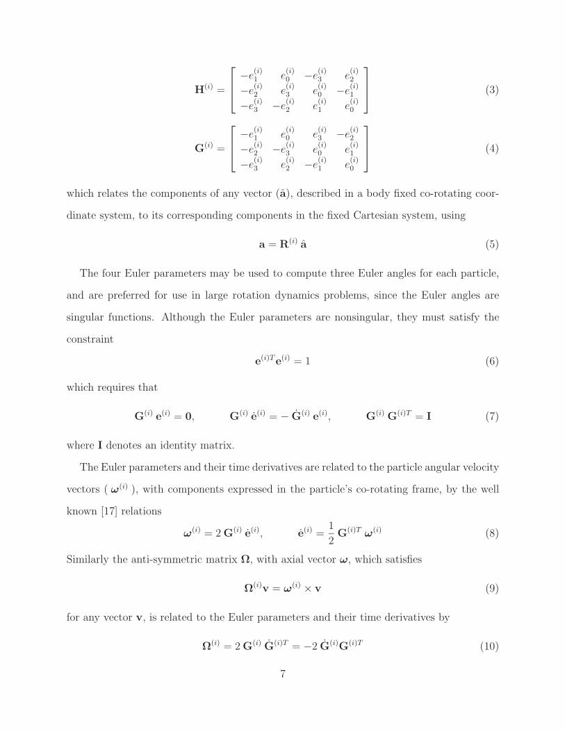
which relates the components of any vector (a), described in a body fixed co-rotating coor-

dinate system, to its corresponding components in the fixed Cartesian system, using

a = R(i) a (5)

The four Euler parameters may be used to compute three Euler angles for each particle,

and are preferred for use in large rotation dynamics problems, since the Euler angles are

singular functions. Although the Euler parameters are nonsingular, they must satisfy the

constraint

e(i)Te(i) = 1 (6)

which requires that

G(i) e(i) = 0, G(i) e(i) = − G(i) e(i), G(i) G(i)T = I (7)

where I denotes an identity matrix.

The Euler parameters and their time derivatives are related to the particle angular velocity

vectors ( ω(i) ), with components expressed in the particle’s co-rotating frame, by the well

known [17] relations

ω(i) = 2 G(i) e(i), e(i) =1

2G(i)T ω(i) (8)

Similarly the anti-symmetric matrix Ω, with axial vector ω, which satisfies

Ω(i)v = ω(i) × v (9)

for any vector v, is related to the Euler parameters and their time derivatives by

Ω(i) = 2 G(i) G(i)T = −2 G(i)G(i)T (10)

7

The next section presents a density interpolation associated with the particles just de-

scribed, and defines Lagrangian finite elements whose nodal coordinates are components of

the particle center of mass position vectors.

DENSITY INTERPOLATION AND FINITE ELEMENTS

In the material reference configuration, the ellipsoidal particles are arranged in a packing

scheme defined by a mapping from a body centered cubic unit cell, the mapping composed

of stretchings in three orthogonal directions, those directions aligned with the principal axes

of the ellipsoids. The density interpolation for compressed states is

ρ(i) = ρ(i)o +

n∑j = 1

ρ(j)o W (i,j) (11)

where ρ(i) is the continuum density at the centroid of the ith particle, ρ(i)o is the reference

density for the ith particle, and W (i,j) is the interpolation kernel

W (i,j) =1

8(1 − δij)

[(1

ζ(i,j)

)3

− 1

]u

(ξ(i,j)

)(12)

ξ(i,j) =

(α + β

2

) (ρ

(i)o

ρ(i)

) 13

− ζ(i,j) (13)

The symbols δij and u denote respectively the Dirac delta function and the unit step function

u(x) =

0, x ≤ 01, x > 0

(14)

The constants α and β are effective separation distances, in a unit cell, measured respectively

between body centered particles and between a body centered particle and a particle located

at a cell vertex

α =(π

3

) 13, β =

√3

2

(π

3

) 13

(15)

Note that the lead coefficient in the expression for W (i,j) is due to the presence of eight

nearest neighbors in the reference configuration.

8

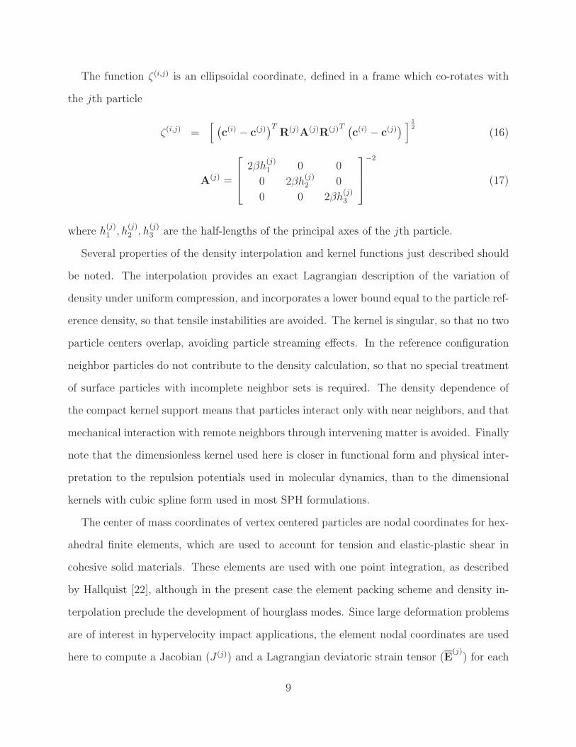
The function ζ(i,j) is an ellipsoidal coordinate, defined in a frame which co-rotates with

the jth particle

ζ(i,j) =[ (

c(i) − c(j))T

R(j)A(j)R(j)T(c(i) − c(j)

) ] 12

(16)

A(j) =

2βh

(j)1 0 0

0 2βh(j)2 0

0 0 2βh(j)3

−2

(17)

where h(j)1 , h

(j)2 , h

(j)3 are the half-lengths of the principal axes of the jth particle.

Several properties of the density interpolation and kernel functions just described should

be noted. The interpolation provides an exact Lagrangian description of the variation of

density under uniform compression, and incorporates a lower bound equal to the particle ref-

erence density, so that tensile instabilities are avoided. The kernel is singular, so that no two

particle centers overlap, avoiding particle streaming effects. In the reference configuration

neighbor particles do not contribute to the density calculation, so that no special treatment

of surface particles with incomplete neighbor sets is required. The density dependence of

the compact kernel support means that particles interact only with near neighbors, and that

mechanical interaction with remote neighbors through intervening matter is avoided. Finally

note that the dimensionless kernel used here is closer in functional form and physical inter-

pretation to the repulsion potentials used in molecular dynamics, than to the dimensional

kernels with cubic spline form used in most SPH formulations.

The center of mass coordinates of vertex centered particles are nodal coordinates for hex-

ahedral finite elements, which are used to account for tension and elastic-plastic shear in

cohesive solid materials. These elements are used with one point integration, as described

by Hallquist [22], although in the present case the element packing scheme and density in-

terpolation preclude the development of hourglass modes. Since large deformation problems

are of interest in hypervelocity impact applications, the element nodal coordinates are used

here to compute a Jacobian (J (j)) and a Lagrangian deviatoric strain tensor (E(j)

) for each

9

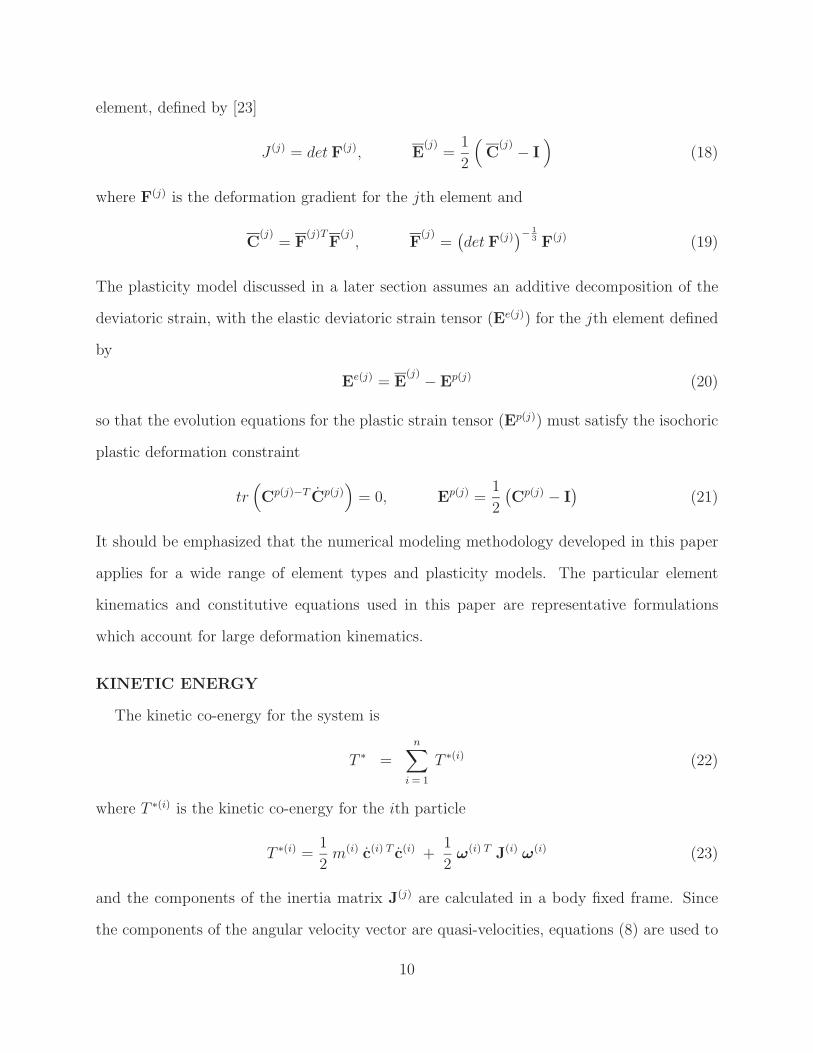
element, defined by [23]

J (j) = det F(j), E(j)

=1

2

(C

(j) − I)

(18)

where F(j) is the deformation gradient for the jth element and

C(j)

= F(j)T

F(j)

, F(j)

=(det F(j)

)− 13 F(j) (19)

The plasticity model discussed in a later section assumes an additive decomposition of the

deviatoric strain, with the elastic deviatoric strain tensor (Ee(j)) for the jth element defined

by

Ee(j) = E(j) − Ep(j) (20)

so that the evolution equations for the plastic strain tensor (Ep(j)) must satisfy the isochoric

plastic deformation constraint

tr(Cp(j)−T Cp(j)

)= 0, Ep(j) =

1

2

(Cp(j) − I

)(21)

It should be emphasized that the numerical modeling methodology developed in this paper

applies for a wide range of element types and plasticity models. The particular element

kinematics and constitutive equations used in this paper are representative formulations

which account for large deformation kinematics.

KINETIC ENERGY

The kinetic co-energy for the system is

T ∗ =n∑

i = 1

T ∗(i) (22)

where T ∗(i) is the kinetic co-energy for the ith particle

T ∗(i) =1

2m(i) c(i) T c(i) +

1

2ω(i) T J(i) ω(i) (23)

and the components of the inertia matrix J(j) are calculated in a body fixed frame. Since

the components of the angular velocity vector are quasi-velocities, equations (8) are used to

10

rewrite the second term

T ∗(i) =1

2m(i) c(i) T c(i) + 2 e(i) TG(i) TJ(i) G(i) e(i) (24)

which identifies the center of mass coordinates and the Euler parameters as generalized

coordinates in Lagrange’s equations. Note that the relations (7) allow the rotational kinetic

co-energy to be expressed as

T∗(i)rot = 2 e(i) T G(i) TJ(i)G(i) e(i) (25)

so that the generalized force associated with the Euler parameter dependence of the kinetic

co-energy is

k(i) =∂T ∗(i)

∂e(i)= 4 G(i) TJ(i)G(i) e(i) (26)

The next section develops a potential energy expression for the particle-element system.

POTENTIAL ENERGY

The potential energy of the particle-element system is the sum of the particle internal

energies and the element stored energies due to tension and elastic shear, and has the general

form

V =n∑

i = 1

m(i) u(i) +ne∑

j = 1

(U ten(j) + Udev(j) + Upen(j)

)(27)

where u(i) is an internal energy per unit mass, ne is the number of elements, U ten(j) is a

stored energy in tension, Udev(j) is a stored energy in shear, and Upen(j) is a penalty energy

used to position the body centered particle in each element. The particle internal energy

density is determined by the mass density and entropy density (s(i))

u(i) = u(i)(ρ(i), s(i)

), s(i) =

S(i)

m(i)(28)

where S(i) is the total entropy of the ith particle. The functional form of the internal energy

per unit mass depends on the equation of state, and it is not unusual in such calculations to

11

rely upon tabular data [24]. In any case, the extensive state variables which determine the

particle internal energy are

u(i) = u(i)(c(j), e(j), S(i)

)(29)

The form of the element stored energy functions depends upon the constitutive assump-

tions. Although the general method developed here admits a wide range of constitutive

models, simple forms are assumed here, and are described as follows. The stored energy in

tension is

U ten(j) =1

2(1 − D(j)) κ(j) V (j)

o (J (j) − 1)2 u(J (j) − 1) (30)

where κ(j) is a bulk modulus, D(j) is the normal damage, and V(j)o is the element reference

volume. The stored energy in shear is

Udev(j) = (1 − d(j)) µ(j) V (j)o tr

(Ee(j)TEe(j)

)(31)

where µ(j) is a shear modulus and d(j) is the deviatoric damage. The penalty function is

Upen(j) =1

2(1 − D(j)) K(j) (c(j) − c(j))2 (32)

where c(j) is the center of mass position vector for the body centered particle of the jth

element, c(j) is the average of the center of mass position vectors for the vertex centered

particles (the element nodes), and the penalty stiffness is

K(j) = E(j)V (j)o

13 (33)

where E(j) is Young’s modulus for the element. The damage variables are used to model the

loss of cohesion due to element failure, and are discussed in the next section.

The preceding constitutive assumptions combine with the element kinematic relations

J (j) = J (j)(c(i)

), Ee(j) = Ee(j)

(c(i),Ep(j)

)(34)

to yield the following state variable dependence for the system potential energy

V = V(c(i), e(i), S(i),Ep(j), D(j), d(j)

)(35)

12

The listed arguments, which include the particle entropies, are by definition Lagrangian

generalized coordinates.

The system potential energy function defines the conservative generalized forces

∂V

∂c(i)= g(i),

∂V

∂e(i)= M(i),

∂V

∂S(i)= θ(i) (36)

where θ(i) is a particle temperature, and g(i) and M(i) are forces and torques which act on

the ellipsoidal particles. The energy conjugates for the dissipative state variables define a

deviatoric stress

S(j) = − 1

V(j)o

∂V

∂Ep(j)(37)

as well as the energy release rates

ΓD(j) = − ∂V

∂D(j), Γd(j) = − ∂V

∂d(j)(38)

The next section discusses evolution equations for the dissipative state variables.

PLASTICITY AND DAMAGE MODELS

The evolution equations for the plastic strain tensor and continuum damage variables will

serve as nonholonomic constraints on the system level Lagrange equations. As discussed in

the last section, the general formulation developed here admits a wide range of constitutive

models. The relatively simple dissipative constitutive models assumed here are described

in this section. The plasticity model is adapted from Fahrenthold and Horban [25], and

represents the simplest possible accommodation of the isochoric deformation constraint (21).

The damage evolution relations are adapted from the Eulerian hydrocode work of Silling [26].

The flow rule for the plastic strain is

Ep(j) =λ(j)

Π(j)(Cp(j) W(j) + W(j) Cp(j)) (39)

W(j) = Cp(j) Sp(j) + Sp(j) Cp(j) − 1

3tr

(Cp(j) Sp(j) + Sp(j) Cp(j)

)I (40)

where λ(j) is a scalar multiplier and

Π(j) = (1 + η(j)εp(j))N(j)

[1

2tr

(W(j)TW(j)

)]1/2

(41)

13

εp(j) =

[1

2tr

(Ep(j)T Ep(j)

)]1/2

(42)

with η(j) a strain hardening modulus, N (j) a strain hardening exponent, and εp(j) the accu-

mulated plastic strain. The effective stress tensor which appears in the flow rule is

Sp(j) = (1 + η(j)εp(j))−N(j)

S(j), S(j) = − 1

V(j)o

∂V

∂Ep(j)= (1 − d(j)) 2 µ(j) Ee(j) (43)

where the indicated deviatoric stress is power density conjugate to the plastic strain rate, in

the entropy equality for the solid medium.

The yield condition is

f (j) = τ (j) − Y (j), τ (j) =

[1

2tr

(Sp(j)TSp(j)

)]1/2

(44)

where τ (j) is the second invariant of the effective stress. The yield stress Y is

Y (j) = Y(j)0 (1 − d(j))

(1 − γ(j)θH(j)

)(45)

where Y(j)0 is the reference yield stress, γ(j) is a thermal softening modulus, and θH(j) is the

maximum historical homologous temperature. The plastic strain increment at each time

step is determined using a one step iteration procedure [22] with

∆λ(j) =(τ (j) − Y (j)) u(τ (j) − Y (j))

(1 − d(j)) 2 µ(j)(46)

The final evolution equations for the plastic strain have the functional form

Ep(j) = Ep(j)(c(i), S(i),Ep(j), d(j)

)(47)

and are nonholonomic constraints on the particle-element model.

Hypervelocity impact problems normally involve perforation and fragmentation effects, so

that the ability to model such physics is essential. In the present case normal and deviatoric

damage variables are introduced, to model the transition from a cohesive solid, characterized

by intact finite elements, to a comminuted medium, described by the free flow of particles.

14

Free particles interact with cohesive material and with other fragments under general contact-

impact loads.

The damage evolutions applied here are

D(j) =Λ(j)

n ∆tu(1 − D(j)), d(j) =

Λ(j)

n ∆tu(1 − d(j)) (48)

where ∆t is the time step, n is the number of time steps used to model the transition from

an intact to a failed element, and

Λ(j) = max u(εp(j) − εp(j)f ), u(θ(j)

max − θ(j)m ), u(J (j)

c − J(j)min), u(σ(j)

max − σ(j)s ) (49)

The function just defined initiates damage evolution in an element when when the accumu-

lated plastic strain εp(j), maximum temperature θmax, minimum element Jacobian J(j)min, or

maximum eigenvalue of the deviatoric stress σ(j)max reach corresponding critical values for the

failure strain (εp(j)f ) , melt temprature (θ

(j)m ), maximum compression (J

(j)c ), or spall stress

(σ(j)s ). More sophisticated damage evolution relations may be introduced without change

to the general modeling framework. The damage evolution equations are nonholonomic

constraints which apply to the system level Lagrange equations.

ARTIFICIAL VISCOSITY AND HEAT DIFFUSION

The shock physics problems of interest here call for the introduction of artificial viscosity

and artificial heat diffusion effects. The standard formulation used here takes the viscosity

force fv(i) on the ith particle to be

fv(i) =n∑

j = 1

ν(i,j) max(0, v(i,j)

)r(i,j), r(i,j) =

(c(i) − c(j)

)| c(i) − c(j) | (50)

where the velocity difference v(i,j) is positive for converging particles

v(i,j) = − (c(i) − c(j)

) · r(i,j) (51)

The damping coefficient ν(i,j) is

ν(i,j) =1

2

(ρ(i) c(i)

s V (i)o

23 + ρ(j) c(j)

s V (j)o

23

) [co +

2 c1|v(i,j)|(c

(i)s + c

(j)s )

]u(1 − ζ(i,j)) (52)

15

where c(i)s is the sound speed for the ith particle and the parameters co and c1 are dimen-

sionless linear and quadratic numerical viscosity coefficients.

The numerical heat diffusion model assumed here takes the thermal power flow for the

ith particle to be

Qcon(i) =n∑

j = 1

R(i,j) ( θ(i) − θ(j) ) (53)

R(i,j) =1

2

(ρ(i) c(i)

s c(i)v V (i)

o

23 + ρ(j) c(j)

s c(j)v V (j)

o

23

)ko u(1 − ζ(i,j)) (54)

where c(i)v is the specific heat for the ith particle and the parameter ko is a dimensionless

numerical heat diffusion coefficient.

ENTROPY EVOLUTION EQUATIONS

The introduction of entropy state variables, which facilitates the use of an energy based

modeling approach, means that the conservation of energy relations normally incorporated

in shock physics models are replaced here by evolution equations for the particle entropies.

These evolution equations are

S(i) = Sirr(i) − Scon(i) (55)

where the irreversible entropy production (Sirr(i)) is due to plastic deformation, damage

evolution, and viscous disspation

Sirr(i) = θ(i)−1

[fv(i)T c(i) +

ne∑j = 1

φ(i,j)

ΓD(j)D(j) + Γd(j)d(j) + V (j)o tr

(S(j)T Ep(j)

)](56)

and φ(i,j) is the fraction of the dissipation in element j associated with the ith particle. The

conduction entropy flow (Scon(i)) is due to artificial heat diffusion

Scon(i) = θ(i)−1 Qcon(i) =n∑

j = 1

R(i,j) ( 1 − θ(j)

θ(i)) (57)

Since the dissipated energy is not lost but rather transduced to the thermal domian, the en-

tropy evolution equations are nonholonomic constraints in the thermomechanical Lagrangian

formulation.

16

VIRTUAL WORK

Although external loads are normally not considered in hypervelocity impact applications,

for completeness this section develops a virtual work expression. The virtual work for the

system is a summation over the particles

δW =n∑

i = 1

δW (i) (58)

In this case the particle angular velocities are the time derivatives of rotational quasi-

coordinates (q(i))

q(i) = ω(i) (59)

so that the virtual work for the ith particle is

δW (i) = f (i)T δc(i) + T(i)T δq(i) (60)

where f (i) and T(i) are externally applied forces and torques. In view of equation (8), virtual

changes in the quasi-coordinates and the Euler parameters are related by

δq(i) = 2 G(i) δe(i) (61)

so that the particle virtual work expression is

δW (i) = f (i)T δc(i) + 2[G(i)TT(i)

]Tδe(i) (62)

The coefficients of the virtual changes in the generalized coordinates are by definition gen-

eralized nonconservative forces in the system level Lagrange equations.

LAGRANGE’S EQUATIONS

The stored energy functions, constraint equations, and virtual work expression developed

in the preceding sections may be combined with the canonical Lagrange equations, to obtain

an ODE model for the particle-element system.

17

The canonical Lagrange equations are

d

dt

(∂T ∗

∂c(i)

)− ∂T ∗

∂c(i)+

∂V

∂c(i)= Qc(i) (63)

d

dt

(∂T ∗

∂e(i)

)− ∂T ∗

∂e(i)+

∂V

∂e(i)= Qe(i) (64)

∂V

∂S(i)= Qs(i),

∂V

∂Ep(j)= Qp(j) (65)

∂V

∂d(j)= Qd(j),

∂V

∂D(j)= QD(j) (66)

where Qc(i), Qe(i), Qs(i), Qd(i), QD(i), and Qp(j) are generalized forces determined by the

constraints and the virtual work. Note that the rate form of the Euler parameter constraint

for the ith particle is

e(i)Te(i) = 0 (67)

Introducing a Lagrange multiplier γe(i) for each Euler parameter constraint as well as La-

grange multipliers γs(i), γd(i), γD(i), and Xp(i) for the entropy, normal damage, deviatoric

damage, and plastic strain evolutions equations, the generalized nonconservative forces are

found to be

Qc(i) = f (i) − γs(i)

θ(i)fv(i) (68)

Qe(i) = 2 G(i)TT(i) + γe(i)e(i) (69)

Qs(i) = γ(i) (70)

Qd(j) = γd(j) −n∑

i = 1

γs(i)

θ(i)φ(i,j) Γd(j) (71)

QD(j) = γD(j) −n∑

i = 1

γs(i)

θ(i)φ(i,j) ΓD(j) (72)

Qp(j) = Xp(j) −n∑

i = 1

γs(i)

θ(i)φ(i,j) V (j)

o S(j) (73)

18

If these results and the degenerate Lagrange equations (65) and (66) are combined with the

previously derived expression for the kinetic co-energy, the momentum balance relations take

the form

d

dt

(m(i) c(i)

)+

∂V

∂c(i)= f (i) − fv(i) (74)

d

dt

(4 G(i) TJ(i) G(i) e(i)

) − k(i) +∂V

∂e(i)= 2 G(i)TT(i) + γe(i)e(i) (75)

Introducing the momentum variables

p(i) = m(i) c(i) , h(i) = J(i) ω(i) (76)

and premultiplying the angular momentum balance expression (75) by 12G(i), which [using

equation (7)] removes the last term, yields the final state space formulation

p(i) = −g(i) − fv(i) + f (i) (77)

h(i) = −Ω(i)h(i) − 1

2G(i)M(i) + T(i) (78)

c(i) = m(i)−1 p(i) (79)

e(i) =1

2G(i)TJ(i)−1h(i) (80)

Augmented by the evolution equations for S(i), D(j), d(j), and Ep(j), these are explicit first

order equations for the particle-element system. With appropriate initial conditions they

may be integrated to obtain solutions for a wide range of hypervelocity impact problems.

EXAMPLE SIMULATIONS

This section compares the results of simulations performed using a numerical implementa-

tion [27] of the model developed here, to published experimental results for two hypervelocity

impact problems. The simulations employed a Mie-Grunsisen equation of state and

co = 0.001, c1 = 0.0, ko = 0.1, εpf = 1.0 (81)

19

with material properties taken from Steinberg [28].

The first example involves the impact of a uranium alloy rod on a steel plate, 0.64 cm in

thickness, in an experiment described by Hertel [29]. The cylindrical projectile is 0.767 cm

in diameter, with a length to diameter ratio of ten, and impacts the plate at an obliquity of

73.5 degrees and a velocity of 1.21 kilometers per second. The velocity of the target plate is

0.217 kilometers per second. The simulation employed 712,929 particles, with the projectile

composed of spherical particles and the target plate composed of ellipsoidal particles with

aspect ratios of 1.5:1.5:1.0. Figure 1 shows an element plot of the initial configuration, while

Figure 2 shows a particle plot of the simulation results at 100 microseconds after impact.

The simulation results for the rod erosion (27.5 percent) and residual rod velocity (1.10

km/s) show good agreement with the corresponding experimental values (27.6 percent and

1.07 km/s).

The second example involves the impact of a tungsten rod on a steel plate, 0.95 cm in

thickness, in an experiment described by Yatteau et al. [30]. The cylindrical projectile is

0.475 cm in diameter, with a length to diameter ratio of twenty, and impacts the plate at

an obliquity of 75 degrees and a velocity of 1.83 kilometers per second. The target plate

is stationary. The simulation employed 671,176 particles, with the projectile composed of

spherical particles and the target plate composed of ellipsoidal particles with aspect ratios of

1.5:1.5:1.0. Figure 3 shows an element plot of the initial configuration, while Figure 4 shows

a particle plot of the simulation results at 150 microseconds after impact. The simulation

results for the rod erosion (37.9 percent) and residual rod velocity (1.60 km/s) show good

agreement with the corresponding experimental values (40 percent and 1.78 km/s).

In the preceding problems the vast majority of the particles are associated with the target

plates, so that the use of ellipsoidal particles reduces the total particle count by a factor of

approximately 2.25, equal to the product of the three indicated aspect ratios. It should be

noted that the computational advantages of a reduced particle count can in part be offset

by an increase in the average number of nominal neighbors per particle. This increase is

20

due to the fact that the neighbor search for each particle must consider a spatial volume

proportional to the cube of the major ellipsoidal axis, despite the fact that a closer approach

without contact can occur when particle minor axes are appropriately aligned. Experience to

date indicates that the use of ellipsoidal particles leads to a reduction in memory requirements

which is proportional to the reduction in particle count, but to a cpu time requirement similar

to that measured in corresponding simulations with spherical particles.

CONCLUSION

The present paper has developed an ellipsoidal particle-finite element method for hyper-

velocity impact problems, and demonstrated its use in the simulation of three dimensional

impact experiments. The hybrid particle-element kinematic scheme allows for the use of

true Lagrangian strength models, while incorporating a completely general description of

contact-impact effects. Tensile instability, numerical fracture, and angular momentum bal-

ance problems, often associated with particle formulations, are avoided. Material remaps,

mass or energy discard, slideline algorithms, and adaptive mesh refinement, often associated

with continuum models, are also avoided. Derivation of the model is based on a thermome-

chanical form of Lagrange’s equations, with entropy variables as generalized coordinates. The

use of an energy based modeling approach facilitates the systematic integration of diverse

particle based and element based interpolations. Work to date suggests that the method pro-

vides a numerically robust and accurate approach to the simulation of hypervelocity impact

problems.

ACKNOWLEDGEMENTS

This work was supported by NASA Johnson Space Center (NAG9-1244), the National

Science Foundation (CMS99-12475), and the State of Texas Advanced Research Program

(003658-0709-1999). Computer time support was provided by the NASA Advanced Super-

computing Division (ARC) and the Texas Advanced Computing Center (UTA).

21

REFERENCES

[1] Anderson CE. An overview of the theory of hydrocodes. International Journal of Impact

Engineering, 1987; 5: 33-60.

[2] McGlaun JM, Thompson SL, Elrick MG. CTH: A three dimensional shock wave physics code.

International Journal of Impact Engineering, 1990; 10: 351-360.

[3] Wallin BK, Tong C, Nichols AL, Chow ET. Large multiphysics simulations in ALE3D.

Presented at the Tenth SIAM Conference on Parallel Processing for Scientific Computing,

Portsmouth, Virginia, March 12-14, 2001.

[4] Faraud M, Destefanis R, Palmieri D, Marchetti M. SPH Simulations of debris impacts using

two different computer codes. International Journal of Impact Engineering, 1999; 23: 249-

260.

[5] Hayhurst CJ, Livingstone IHG, Clegg, RA, Destefanis R, Faraud M. Ballistic limit evalu-

ation of advanced shielding using numerical simulations. International Journal of Impact

Engineering, 2001; 26: 309-320.

[6] Fahrenthold EP, Horban BA. An improved hybrid particle-element method for hypervelocity

impact simulation. International Journal of Impact Engineering, 2001; 26: 169-178.

[7] Fahrenthold EP. Numerical simulation of impact on hypervelocity shielding. Proceedings

of the Hypervelocity Shielding Workshop, 1998, Galveston, Texas, pp. 47-50.

[8] Rapaport DC. Molecular dynamics simulation using quaternions. Journal of Computational

Physics, 1985; 41: 306-314.

[9] Shapiro PR, Martel H, Villumsen JV, Owen JM. Adaptive smoothed particle hydrodynamics

with application to cosmology: methodology. The Astrophysical Journal Supplement Series,

1996; 103: 269-330.

[10] Owen JM, Villumsen JV, Shapiro PR, Martel H. Adaptive smoothed particle hydrodynam-

ics with application to cosmology: methodology II. The Astrophysical Journal Supplement

Series, 1998; 116: 155-209.

22

[11] Benson DJ. Computational methods in Lagrangian and Eulerian hydrocodes. Computer

Methods in Applied Mechanics and Engineering, 1992; 99: 235-394.

[12] Carroll DE, Hertel ES, Trucano TG. Simulation of armor penetration by tungsten

rods: ALEGRA validation report, 1997, SAND97-2765, Sandia National Laboratories.

[13] Stellingwerf RF, Wingate CA. Impact modeling with smooth particle hydrodynamics. Inter-

national Journal of Impact Engineering, 1993; 14: 707-718.

[14] Johnson GR, Petersen EH, Stryk RA. Incorporation of an SPH option into the EPIC code

for a wide range of high velocity impact computations. International Journal of Impact

Engineering, 1993; 14: 385-394.

[15] Belytschko T, Krongauz Y, Organ D, Fleming M, Krysl P. Meshless methods: an overview

and recent developments. Computer Methods in Applied Mechanics and Engineering, 1996;

139: 3-47.

[16] Hayhurst CJ, Livingstone IH, Clegg RA, Fairlie GE, Hiermaier SH, Lambert M. Numerical

simulation of hypervelocity impacts on aluminum and Nextel/Kevlar Whipple shields. Pro-

ceedings of the Hypervelocity Shielding Workshop, 1998, Galveston, Texas, pp.

61-72.

[17] Haim Baruh. Analytical Dynamics, 1999, McGraw Hill, New York.

[18] C.O. Chang and C.S. Chou. Design of a viscous ring nutation damper for a freely precessing

body. Journal of Guidance, Control and Dynamics, 1991; 14: 1136-1144.

[19] P.E. Nikravesh, R.A. Wehage, and O.K. Kwon. Euler parameters in computational kinematics

and dynamics. part 1. Journal of Mechanisms, Transmissions and Automation Design, 1985;

107: 358-365.

[20] P.E. Nikravesh, O.K. Kwon, and R.A. Wehage. Euler parameters in computational kinematics

and dynamics. part 2. Journal of Mechanisms, Transmissions and Automation Design, 1985;

107: 366-369.

23

[21] Fahrenthold EP, Shivarama R. Extension and validation of a hybrid particle-element method

for hypervelocity impact simulation. International Journal of Impact Engineering, accepted

for publication.

[22] Hallquist JO. Theoretical Manual for DYNA3D, 1983, Lawrence Livermore National

Laboratory, Livermore, California.

[23] Lubliner J. Plasticity theory, 1990, Macmillan, New York

[24] Lyon SP, Johnson JD, editors. SESAME: The Los Alamos National Laboratory

Equation of State Database, LA-UR-92-3407, Los Alamos National Laboratory, Los

Alamos, New Mexico.

[25] Fahrenthold EP, Horban BA. Thermodynamics of continuum damage and fragmentation mod-

els for hypervelocity impact. International Journal of Impact Engineering, 1997; 20: 241-252.

[29] Silling SA. CTH Reference Manual: Johnson-Holmquist Ceramic Model, 1992,

SAND92-0576, Sandia National Laboratories.

[27] Fahrenthold EP. User’s Guide for EXOS, 2001, University of Texas, Austin.

[28] Steinberg DJ. Equation of State and Strength Properties of Selected Materials,

1996, Lawrence Livermore National Laboratory, UCRL-MA-106439.

[29] Hertel ES. A Comparison of the CTH Hydrodynamics Code With Experimental

Data, 1992, SAND92-1879, Sandia National Laboratories.

[30] Yatteau JD, Recht GW, Edquits KT. Transverse loading and response of long rod penetrators

during high velocity plate perforation. International Journal of Impact Engineering, 1999;

23: 967-980.

24

LIST OF FIGURES

Figure 1. Uranium alloy long rod impact on a steel plate, element plot of the initial

configuration

Figure 2. Uranium alloy long rod impact on a steel plate, particle plot at 100 microsec-

onds after impact

Figure 3. Tungsten long rod impact on a steel plate, element plot of the initial config-

uration

Figure 4. Tungsten long rod impact on a steel plate, particle plot at 150 microseconds

after impact

25

Figure 1: Uranium alloy long rod impact on a steel plate, element plot of the initial config-uration

26

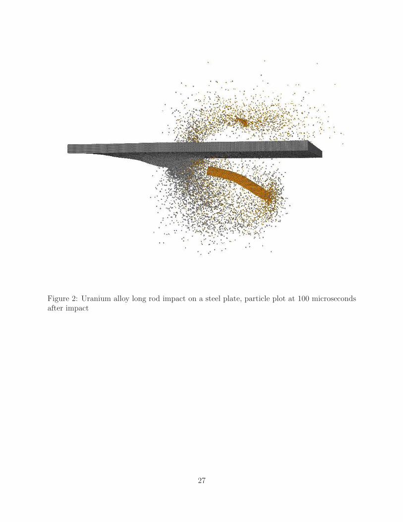
Figure 2: Uranium alloy long rod impact on a steel plate, particle plot at 100 microsecondsafter impact

27

Figure 3: Tungsten long rod impact on a steel plate, element plot of the initial configuration

28

Figure 4: Tungsten long rod impact on a steel plate, particle plot at 150 microseconds afterimpact

29