chapter 07: modal analysis - pudn.comsummarizing the modal analysis method of analyzing ... sdof...

CHAPTER 7

MODAL ANALYSIS

7.1 Introduction

In Chapter 2 we systematically defined the equations of motion for a multi dof (mdof) system and transformed to the “s” domain using the Laplace transform. Chapter 3 discussed frequency responses and undamped mode shapes.

Chapter 5 discussed the state space form of equations of motion with arbitrary damping. It also covered the subject of complex modes. Heavily damped structures or structures with explicit damping elements, such as dashpots, result in complex modes and require state space solution techniques using the original coupled equations of motion.

Lightly damped structures are typically analyzed with the “normal mode” method, which is the subject of this chapter. The ability to think about vibrating systems in terms of modal properties is a very powerful technique that serves one well in both performing analysis and in understanding test data. The key to normal mode analysis is to develop tools which allow one to reconstruct the overall response of the system as a superposition of the responses of the different modes of the system. In analysis, the modal method allows one to replace the n-coupled differential equations with n-uncoupled equations, where each uncoupled equation represents the motion of the system for that mode of vibration. If natural frequencies and mode shapes are available for the system, then it is easy to visualize the motion of the system in each mode, which is the first step in being able to understand how to modify the system to change its characteristics.

Summarizing the modal analysis method of analyzing linear mechanical systems and the benefits derived:

1) Solve the undamped eigenvalue problem, which identifies the resonant frequencies and mode shapes (eigenvalues and eigenvectors), useful in themselves for understanding basic motions of the system.

2) Use the eigenvectors to uncouple or diagonalize the original set of coupled equations, allowing the solution of n-uncoupled sdof problems instead of solving a set of n-coupled equations.

© 2001 by Chapman & Hall/CRC

3) Calculate the contribution of each mode to the overall response. This also allows one to reduce the size of the problem by eliminating modes that cannot be excited and/or modes that have no outputs at the desired dof’s. Also, high frequency modes that have little contribution to the system at lower frequencies can be eliminated or approximately accounted for, further reducing the size of the system to be analyzed.

4) Write the system matrix, A, by inspection. Assemble the input and output matrices, B and C, using appropriate eigenvector terms. Frequency domain and forced transient response problems can be solved at this point. If complete eigenvectors are available, initial condition transient problems can also be solved. For lightly damped systems, proportional damping can be added, while still allowing the equations to be uncoupled.

7.2 Eigenvalue Problem

7.2.1 Equations of Motion

We will start by writing the undamped homogeneous (unforced) equations of motion for the model in Figure 7.1. Then we will define and solve the eigenvalue problem.

Figure 7.1: Undamped tdof model.

+ =mz kz 0&& (7.1)

From (2.5) with 1 2k k k= = and c1 = c2 = 0:

m1 m2 m3

k1 k2

z1 z2 z3F1 F2 F3


1 1

2 2

3 3

m 0 0 z k k 0 z 00 m 0 z k 2k k z 00 0 m z 0 k k z 0

− + − − = −

&&

&&

&&

(7.2)

7.2.2 Principal (Normal) Mode Definition

Since the system is conservative (it has no damping), normal modes of vibration will exist. Having normal modes means that at certain frequencies all points in the system will vibrate at the same frequency and in phase, i.e., all points in the system will reach their minimum and maximum displacements at the same point in time. Having normal modes can be expressed as (Weaver 1990):

( ) i ij ti mi i i misin t Im(e )ω +φ= ω + φ =z z z (7.3)

Where:

iz = vector of displacements for all dof’s at the thi frequency

miz = the thi eigenvector, the mode shape for the thi resonant frequency

iω = the ith eigenvalue, ith resonant frequency

iφ = an arbitrary initial phase angle

For our tdof system, for the thi frequency, the equation would appear as:

( )1 m1i

2 m2i i i

3 m3i

z zz z sin tz z

= ω + φ

, (7.4)

where the indices in the mkiz term represent the kth dof and the ith mode of the modal matrix mz .

7.2.3 Eigenvalues / Characteristic Equation

Since the equation of motion

0+ =mz kz&& (7.5)


and the form of the motion

( )i mi i i sin t= ω + φz z (7.6)

are known, iz can be differentiated twice and substituted into the equation of motion:

( )2i i mi i i sin t= −ω ω + φz z&& (7.7)

( ) ( )2i mi i i mi i i sin t sin t 0 −ω ω + φ + ω + φ = m z k z (7.8)

Canceling the sine terms:

2i mi mi 0−ω + =mz kz (7.9)

2mi i mi= ωkz mz (7.10)

Equation (7.10) is the eigenvalue problem in nonstandard form, where the standard form is (Strang 1998):

= λAz z (7.11)

The solution of the simultaneous equations which make up the standard form eigenvalue problem is a vector z such that when z is multiplied by A , the product is a scalar multiple of z itself.

The nonstandard problem is “nonstandard” because the mass matrix m falls on the right-hand side. The form of the matrix presents no problem for hand calculations, but for computer calculations it is best transformed to standard form.

Rewriting the nonstandard form eigenvalue problem as a homogeneous equation:

( )2i mi 0− ω =k m z (7.12)

A trivial solution, mi 0=z , exists but is of no consequence. The only possibility for a nontrivial solution is if the determinant of the coefficient matrix is zero (Strang 1998). Expanding the matrix entries:


2i mi

k k 0 m 0 0k 2k k 0 m 0 0

0 k k 0 0 m

− − − − ω = −

z (7.13)

Performing the matrix subtraction:

2i

21 mi

2i

k m k 0k 2k m k 0

0 k k m

− ω − − − ω − = − − ω

z (7.14)

Setting the determinant of the coefficient matrix equal to zero:

2i

2i

2i

k m k 0k 2k m k 0

0 k k m

− ω −− − ω − =

− − ω (7.15)

The determinant results in a polynomial in 2iω , the characteristic equation,

where the roots of the polynomial are the eigenvalues, poles, or resonant frequencies of the system.

( )

3 6 2 4 2 2

2 3 4 2 2 2

m 4km 3k m 0

m 4km 3k m 0

− ω + ω − ω =

ω − ω + ω − =

(7.16a,b)

Two of the roots are at the origin:

1 0ω = (7.17)

Solving for 2ω as a quadratic in (7.16b) above:

( )1

2 2 4 2 4 22

3

4km 16k m 12k m

2m

− ± −ω =

−

2 2

3

4km 2km2m

− ±=−


6k 2k,2m 2m

− −=− −

3k k,m m

= (7.18)

2

3

3kmkm

ω = ±

ω = ± (7.19)

For each of the three eigenvalue pairs, there exists an eigenvector iz , which gives the mode shape of the vibration at that frequency.

7.2.4 Eigenvectors

To obtain the eigenvectors of the system, any one of the degrees of freedom, say z1, is selected as a reference. Then, all but one of the equations of motion is written with that value on the right-hand side:

( )2i mi 0− ω =k m z (7.20)

( )( )

( )

2i

m1i2i m2i

2 m3ii

k m k 0 zk 2k m k z 0

z0 k k m

− ω − − − ω − = − − ω

(7.21)

Expanding the first and second equations, dropping the subscripts “ i ” and “m”:

( )( )

2i 1 2

21 i 2 3

k m z kz 0

kz 2k m z kz 0

− ω − =

− + − ω − = (7.22a,b)

Rewriting with the 1z term on the right-hand side and solving for the ( )2 1z / z ratio from (7.22a):

( )22 i 1kz k m z− = − − ω (7.23)


22 i

1

z k mz k

− ω= (7.24)

Solving for the ( )3 1z / z ratio from (7.22b):

( )2i 2 3 12k m z kz kz− ω − = (7.25)

( )2 32i

1 1

kzz2k m kz z

− ω − =

(7.26)

( )2

2 3ii

1

kzk m2k m kk z

− ω− ω − =

(7.27)

( )( )2 2i i3

21

2k m k mz1

z k

− ω − ω= − (7.28)

2 4 2 23 i i

21

z m 3km kz k

ω − ω += (7.29)

We now have the general equations for the eigenvector values. If a value is chosen for 1z , say 1.0, then the two ratios above can be solved for corresponding values of 2 3z and z for each of the three eigenvalues.

Since at each eigenvalue there are (n+1) unknowns ( )i mi, zω for a system with n equations of motion, the eigenvectors are only known as ratios of displacements, not as absolute magnitudes. For the first mode of our tdof system the unknowns are i m11 m21 m31, z , z and zω and we have only three equations of motion.

Substituting values for the three eigenvalues into the general eigenvector ratio equations above, assuming 1 2m m m 1= = = , 1 2k k k 1= = = :

For mode 1, 21 0ω =

2

1

z k 1z k

= = (7.30)


2 1z z= (7.31)

( )( )32

1

2k kz1 2 1 1

z k= − = − = (7.32)

3 1z z= (7.33)

Arbitrarily assigning z1=1:

1

111

=

z (7.34)

1 1 1

Rigid-Body Mode, 0 rad/sec

Figure 7.2: Mode shape plot for rigid body mode, where all masses move together with no stress in the connecting springs.

For mode 2, 22

km

ω =

2

1

kk mz m 0z k

− = = (7.35)

2z 0= (7.36)

( ) ( )32

1

k k2k m k m2k k 0m mz

1 1 1z k2k

− − − = − = − = − (7.37)


3 1z z= − (7.38)

2

101

= −

z (7.39)

1 -1

Second Mode, Middle Mass Stationary, 1 rad/sec

Figure 7.3: Mode shape plot for second mode, middle mass stationary and the two end masses move out of phase with each other with equal amplitude.

For node 3, 23

3km

ω =

2

1

3kk mz 2km 2z k k

− − = = = − (7.40)

2 1z 2z= − (7.41)

( ) ( ) 23

2 2 21

3k 3k2k m k mk 2k 1m mz 2k 11 1

z k k k

− − − − − − = − = = = (7.42)

3 1z z= (7.43)

3

12

1

= −

z (7.44)


1 1-2

Third Mode, 1.732 rad/sec

Figure 7.4: Mode shape plot for third mode, with two end masses moving in phase with each other and out of phase with the middle mass, which is moving with twice the

amplitude of the end masses.

7.2.5 Interpreting Eigenvectors

For the first mode, if all the masses start with either zero or the same initial velocity and with initial displacements of some scalar multiple of [ ]T1 1 1 , where “T” is the transpose, the system will either remain at rest or will continue moving at that velocity with no relative motion between the masses.

For the second and third modes, if the system is released with zero initial velocities but with initial displacements of some scalar multiple of that eigenvector, then the system will vibrate in only that mode with all the masses reaching their minimum and maximum points at the same point in time.

Any other combination of initial displacements will result in a motion which is a combination of the three eigenvectors.

7.2.6 Modal Matrix

Now that the three eigenvectors have been defined, the modal matrix will be introduced. The modal matrix is an (nxn) matrix with columns corresponding to the n system eigenvectors, starting with the first mode in the first column and so on:


mode: 1 2 3

m11 m12 m13

m m21 m22 m23

m31 m32 m33

z z z DOF1z z z DOF2z z z DOF3

← = ← ←

z (7.45)

1 2 3

↑ ↑ ↑z z z

For our tdof problem:

m

1 1 11 0 21 1 1

= − −

z (7.46)

7.3 Uncoupling the Equations of Motion

At this point the system is well defined in terms of natural frequencies and modes of vibration. If any further information such as transient or frequency response is desired, solving for it would be laborious because the system equations are still coupled. For transient response, the equations would have to be solved simultaneously using a numerical integration scheme unless the problem were simple enough to allow a closed form solution. To calculate the damped frequency response, a complex equation solving routine would have to be used to invert the complex coefficient matrix at each frequency.

In order to facilitate solving for the transient or frequency responses, it is useful to transform the n-coupled second order differential equations to n-uncoupled second order differential equations by transforming from the physical coordinate system to a principal coordinate system. In linear algebra terms, the transformation from physical to principal coordinates is known as a change of basis. There are many options for change of basis, but we will show that when eigenvectors are used for the transformation the principal coordinate system has a physical meaning; each of the uncoupled sdof systems represents the motion of a specific mode of vibration. The n-uncoupled equations in the principal coordinate system can then be solved for the responses in the principal coordinate system using well-known solutions for single degree of freedom systems. The n-responses in the principal coordinate system can then be transformed back to the physical coordinate system to provide the actual


response in physical coordinates. This procedure is shown schematically in Figure 7.5.

PHYSICAL COORDINATES

Coupled Equations of MotionInitial ConditionsForcing Functions

PRINCIPAL COORDINATES

Uncoupled Equations of MotionInitial ConditionsForcing Functions

Solution

PHYSICAL COORDINATES

Solution

Transform

Back-Transform

Figure 7.5: Roadmap for Modal Solution

The procedure above is analogous to using Laplace transforms for solving differential equations, where the differential equation is transformed to an algebraic equation, solved algebraically, and back transformed to get the solution of the original problem.

We now need a means of diagonalizing the mass and stiffness matrices, which will yield a set of uncoupled equations.

The condition to guarantee diagonalization is the existence of n-linearly independent eigenvectors, which is always the case if the mass and stiffness matrices are both symmetric or if there are n-different (nonrepeated) eigenvalues (Strang 1998).

Going back to the original homogeneous equation of motion:

0+ =mz kz&& (7.47)


Having normal modes means that at frequency “i”:

i mi i i sin ( t )= ω + φz z (7.48)

Differentiating twice to get acceleration:

2i i mi i isin ( t )= −ω ω + φz z&& (7.49)

Substituting back into the equation of motion:

{ } { }2i mi i i mi i isin( t ) sin( t ) 0−ω ω + φ + ω + φ =m z k z (7.50)

Canceling sine terms:

2i mi mi 0−ω + =mz kz (7.51)

Rearranging and writing the above equation for both the “ith” and “jth” modes:

2mi i mi= ωkz mz (7.52)

2mj j mj= ωkz mz (7.53)

miz and mjz are the “ith” and “jth” eigenvectors, the “ith” and “jth” columns of the modal matrix.

Premultiplying (7.52) by the transpose of Tmj mj,z z :

T 2 Tmj mi i mj mi= ωz kz z mz (7.54)

Taking the transpose of (7.53), where the transpose of a product is the product of the individual transposes taken in reverse order, i.e., [ ]T T T=AB B A :

T T 2 T Tmj j mj ,= ωz k z m (7.55)

since m and k are symmetrical, T T, and= =m m k k :

T 2 Tmj j mj= ωz k z m (7.56)


Postmultiplying (7.56) by miz

T 2 Tmj mi j mj mi= ωz kz z mz (7.57)

Now, subtracting (7.57) from (7.54):

T 2 Tmj mi i mj miT 2 Tmj mi j mj mi

2 2 Ti j mj mi

( )0 ( )

= ω− = ω

= ω − ω

z kz z mzz kz z mz

z mz (7.58)

When i j=/ , the term ( )2 2i jω − ω cannot be equal to zero, meaning that the

term Tmj miz mz must be equal to zero.

Tmj mi 0=z mz (7.59)

Looking at the sizes of the matrices multiplied:

Tmj

mi

1xnnxnnx1

=

==

zm

z (7.60)

( ) ( ) ( ) ( )1xn x nxn x nx1 1x1 scalar= = (7.61)

Equation (7.59) can be rewritten:

Tmj mi ijm 0= =z mz , (7.62)

where mij is an off-diagonal term in the mass matrix of the principal coordinate system.

The two eigenvectors mjz and miz are said to be orthogonal with respect to m , where orthogonality is defined as the property that causes all the off-diagonal terms in the principal mass matrix to be zero.

Returning to (7.62), for ( )2 2i ji j, 0= ω − ω = . Thus the product T

mi miz mz can

be set equal to any arbitrary constant iim ,, a diagonal term in the principal mass matrix.


Tmi mi iim=z mz (7.63)

This is where various normalization techniques for eigenvectors come into play, discussed in the next section.

The stiffness matrix, k, is normalized in the same manner.

In practice, instead of diagonalizing the mass and stiffness matrices term by term by pre- and postmultiplying by individual eigenvectors, the entire modal matrix is used to diagonalize in one operation using two matrix multiplications:

Tn m m=m z mz (7.64)

Tn m m=k z kz (7.65)

7.4 Normalizing Eigenvectors

Because eigenvectors are only known as ratios of displacements, not as absolute magnitudes, we can choose how to normalize them. Up to now, when calculating eigenvectors we have arbitrarily set the amplitude of the first dof to 1. We will now discuss two of the most commonly used eigenvector normalization techniques. Different normalizing techniques result in different forms of the resulting uncoupled differential equations.

7.4.1 Normalizing with Respect to Unity

One method is to normalize with respect to unity, making the largest element in each eigenvector equal to unity by dividing each column by its largest value. We now add the notation nz , where the “n” refers to a “normalized” modal matrix.

m n

1 1 1 1 1 0.51 0 2 1 0 11 1 1 1 1 0.5

− = − ⇒ = − − −

z z (7.66)

Using the unity normalized modal matrix to transform the mass matrix in two matrix multiplications:


Tn

1 1 1 m 0 0 m m m1 0 1 0 m 0 m 0 m0.5 1 0.5 0 0 m .5m m .5m

= − = − − − − −

z m (7.67)

Tn n n

m m m 1 1 .5 3m 0 0m 0 m 1 0 1 0 2m 0.5m m .5m 1 1 .5 0 0 1.5m

− = = − = − − − −

m z mz (7.68)

Similarly transforming the stiffness matrix:

Tn

1 1 1 k k 0 0 0 01 0 1 k 2k k k 0 k.5 1 .5 0 k k 1.5k 3k 1.5k

− = − − − = − − − − − −

z k (7.69)

Tn n n

0 0 0 1 1 .5 0 0 0k 0 k 1 0 1 0 2k 0

1.5k 3k 1.5k 1 1 .5 0 0 4.5k

− = = − − = − − − −

k z kz (7.70)

Note that the original filled stiffness matrix is now diagonal. Also note that if the diagonal elements of the stiffness matrix (7.70) are divided by the corresponding diagonal elements of the mass matrix (7.69), the three terms are the squares of the respective eigenvalues.

7.4.2 Normalizing with Respect to Mass

Another method is to normalize with respect to mass using the equation:

Tni ni 1.0=z mz , (7.71)

making each diagonal mass term equal 1.0. This is the method used by default in ANSYS.

Once again, note that modal matrix subscript “ni” in niz signifies the normalized ith eigenvector. Each normalized eigenvector is defined as follows:

mi mini 1

T i2mi mi

q= =

z zzz mz

(7.72)


Where qi is defined as:

1n n 2

i mji jk mkij i k 1

q z m z= =

=

∑ ∑ (7.73)

For a diagonal mass matrix, q can be simplified since all the jkm terms are zero:

1n 2

2i k mki

k 1q m z

=

= ∑ (7.74)

Thus, by operating on m by nz ,the mass matrix should be transformed into the identity matrix. Starting with mz and the “q” values from above:

m

1 1 11 0 21 1 1

= − −

z (7.75)

( ) ( ) ( )

( ) ( ) ( )

( ) ( ) ( )

12 2 2 2

1

12 2 2 2

2

12 2 2 2

3

q m 1 m 1 m 1 3m

q m 1 m 0 m 1 2m

q m 1 m 2 m 1 6m

= + + =

= + + − =

= + − + =

(7.76a,b,c)

The modal matrix normalized with respect to mass becomes:

n

1 1 1 1 1 13m 2m 6m 3 2 61 2 1 1 20 03m 6m m 3 61 1 1 1 1 13m 2m 6m 3 2 6

− −= = − −

z (7.77)

Using nz to transform the mass matrix:


Tn

1 1 1 m m mm 0 03m 3m 3m 3m 3m 3m1 1 m m0 00 m 02m 2m 2m 2m1 2 1 m 2m m

0 0 m6m 6m 6m 6m 6m 6m

− − = = − −

z m (7.78)

Tn n n

m m m 1 1 13m 3m 3m 3m 2m 6mm m 1 20 02m 2m 3m 6mm 2m m 1 1 16m 6m 6m 3m 2m 6m

− −= = − −

m z mz (7.79)

n

m m m m m03m 3m 3m m 3 2 m 3 2

m m m m0 02m 2mm 2 3 m 2 3

m 2m m m m0m 3 6 m 3 6 m 3 6 m 2 6 m 6 2

m 2m mm 3 6 m 3 6 m 3 6

m m0m 2 6 m 2 6

m 4m m6m 6m 6m

1 0 00 1 00 0 1

+ + + −

= + − + +

− + + −

− +

+ − + +

=

m

(7.80)

The original mass matrix has been transformed to the identity matrix.

Similarly transforming the stiffness matrix:


Tn

1 1 1 1 1 03 3 3

1 1 10 k 1 2 1m 2 2

1 2 10 1 1

6 6 6

− − = − − − −

z k

1 1 1 2 1 1 103 3 3 3 3 3 3

k 1 1 1 10 0 0 0 0m 2 2 2 2

1 2 1 4 1 2 10 06 6 6 6 6 6 6

− − + − − +

− = + + + + + − − + + − − + +

(7.81)

Tn n n

1 1 10 0 0 3 2 61 1 1 2 k0 0

m2 2 3 63 6 3 1 1 16 6 6 3 2 6

− −= = − −

k z kz (7.82)

n

0 0

k 1 1 1 10m 2 22 3 2 3

3 6 3 3 303 6 3 6 3 6 2 6 6 2

0

1 102 6 2 6

3 12 36 6 6

= − + +

− + − −

+ −

+ +

k

(7.83)


n

0 0 0k0 1 0m

0 0 3

=

k (7.84)

Note that the normalized stiffness matrix is now diagonal and that the diagonal terms are the squares of the corresponding three eigenvalues. The normalized stiffness matrix is also known as the spectral matrix (Weaver 1990).

Because normalizing with respect to mass results in an identity principal mass matrix and squares of the eigenvalues on the diagonal in the principal stiffness matrix, we will use only this normalization in the future. Since we know the form of the principal matrices when normalizing with respect to mass, no multiplying of modal matrices is actually required: the homogeneous principal equations of motion can be written by inspection knowing only the eigenvalues.

7.5 Reviewing Equations of Motion in Principal Coordinates – Mass Normalization

7.5.1 Equations of Motion in Physical Coordinate System

[ ]1 1

2 2

3 3

m 0 0 z k k 0 z0 m 0 z k 2k k z 00 0 m z 0 k k z

− + − − = −

&&

&&

&&

(7.85)

Eigenvalues:

1 0ω = (7.86)

2

3

3kmkm

ω = ±

ω = ± (7.87a,b)

Eigenvectors, normalized with respect to mass:


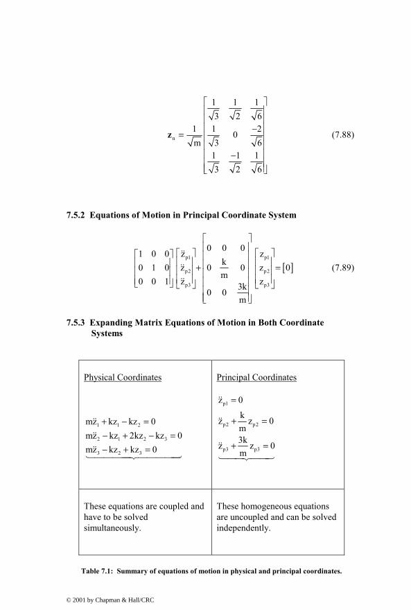
n

1 1 13 2 6

1 1 20m 3 6

1 1 13 2 6

−= −

z (7.88)

7.5.2 Equations of Motion in Principal Coordinate System

[ ]p1 p1

p2 p2

p3 p3

0 0 01 0 0 z zk0 1 0 z 0 0 z 0m

0 0 1 z z3k0 0m

+ =

&&

&&

&&

(7.89)

7.5.3 Expanding Matrix Equations of Motion in Both Coordinate Systems

Physical Coordinates

1 1 2

2 1 2 3

3 2 3

mz kz kz 0mz kz 2kz kz 0mz kz kz 0

+ − =− + − =− + =

&&

&&

&&1444442444443

Principal Coordinates

p1

p2 p2

p3 p3

z 0

kz z 0m3kz z 0m

=

+ =

+ =

&&

&&

&&1442443

These equations are coupled and have to be solved simultaneously.

These homogeneous equations are uncoupled and can be solved independently.

Table 7.1: Summary of equations of motion in physical and principal coordinates.


7.6 Transforming Initial Conditions and Forces

Now that we know how to construct the homogeneous uncoupled equations of motion for the system, we need to know how to transform initial conditions and forces to the principal coordinate system. We can then solve for transient and forced responses in the principal coordinate system using the uncoupled equations.

Starting with the original non-homogeneous equations of motion in physical coordinates:

+ =mz kz F&& (7.90)

Premultiplying by Tnz , the transpose of the modal matrix:

T T Tn n n+ =z mz z kz z F&& (7.91)

Inserting the identify matrix, n n−= 1I z z :

{ {T 1 T 1 Tn n n n n n n

− −+ =z m z z z z k z z z z FI I

&& (7.92)

Rewriting and regrouping terms:

{ {{ {T 1 T 1 Tn n n n n n n

p p p pp

− −+ =z mz z z z kz z z z Fz k z Fm&&

123&&

, (7.93)

where Tn nz mz and T

n nz kz were shown to diagonalize the mass and stiffness matrices in the previous section.

Defining terms:

pm = (nxn) diagonal principal mass matrix

pk = (nxn) diagonal principal stiffness matrix

1n p− =z z z&& && = acceleration vector in principal coordinates

1n p− =z z z = displacement vector in principal coordinates


Tn p=z F F = force vector in principal coordinates

In the previous section, the definitions for accelerations and displacements in physical and principal coordinates were shown to be:

1p n

1p n

−

−

=

=

z z z

z z z

&& && (7.94)

The same relationships hold for initial conditions of displacement and velocity:

1op n o

1op n o

−

−

=

=

z z z

z z z& & (7.95)

In (7.95), opz and opz& are vectors of initial displacements and velocities, respectively, in the principal coordinate system, and oz and oz& are vectors of initial displacements and velocities, respectively, in the physical coordinate system.

Taking the inverse of the modal matrix to convert initial conditions requires that the modal matrix be square, with as many eigenvectors as number of degrees of freedom. We will see in future chapters that there are instances where not all eigenvectors are available. In one case, we may choose to only calculate eigenvalues and eigenvectors up to a certain frequency in order to save calculation time or because the problem only requires knowledge of response in a certain frequency range. In another case, we may build a “reduced” model where only the most significant modes are retained. Fortunately, a large majority of real life problems involve zero initial conditions.

7.7 Summarizing Equations of Motion in Both Coordinate Systems

The two sets of equations, in physical and principal coordinates, are shown in Table 7.2:


Physical Coordinates Principal Coordinates

1 1 2 1

2 1 2 3 2

3 2 3 3

1 2 3 1 2 3

mz kz kz Fmz kz 2kz kz Fmz kz kz FIC 's : z , z , z , z , z , z

+ − =− + − =− + =

&&

&&

&&

& & &

p1 p1

p2 p2 p2

p3 p3 p3

p1 p2 p3 p1 p2 p3

z F

kz z Fm3kz z Fm

IC 's : z , z , z , z , z , z

=

+ =

+ =

&&

&&

&&

& & &

Table 7.2: Summary of equations of motion in physical and principal coordinates.

The variables in physical coordinates are the positions and velocities of the masses. The variables in principal coordinates are the displacements and velocities of each mode of vibration.

The equations in principal coordinates can be easily solved, since the equations are uncoupled, yielding the displacements. We now need to back transform the results in the principal coordinate system to the physical coordinate system to get the final answer.

7.8 Back-Transforming from Principal to Physical Coordinates

We showed previously that the relationship between physical and principal coordinates is:

1n p− =z z z (7.96)

Premultiplying by nz :

1n n n p( )− =z z z z z

I123

(7.97)

n p=z z z (7.98)

Thus, the displacement vector in physical coordinates is obtained by premultiplying the vector of displacements in principal coordinates by the normalized modal matrix nz .


Similarly for velocity:

n p=z z z& & (7.99)

7.9 Reducing the Model Size When Only Selected Degrees of Freedom are Required

So far we have hinted at the fact that only portions of the eigenvector matrix are needed if selected dof’s have forces applied and other (or the same) dof’s are needed for output. This section will show how the reduction in dof’s occurs. This reduction is one of the key steps to be used later in the book when we cover how to reduce the size of models derived from large finite element simulations.

Reviewing the steps in the modal solution, starting with the equations of motion and initial conditions in physical coordinates:

1 1 2 1

2 1 2 3 2

3 2 3 3

1 2 3 1 2 3

mz kz kz Fmz kz 2kz kz F

mz kz kz F

Initial Conditions : z , z , z , z , z , z 0

+ − =− + − =

− + =

=

&&

&&

&&

& & &

(7.100)

Solve for eigenvalues: 1 2 3, ,ω ω ω

Solve for eigenvectors, normalize with respect to mass and form the modal matrix from columns of eigenvectors:

n11 n12 n13

n n21 n22 n23

n31 n32 n33

z z zz z zz z z

=

z (7.101)

Transform forces from physical to principal coordinates:

Tp n=F z F (7.102)

Write the equations of motion in principal coordinates:


p1 p1

2p2 2 p2 p2

2p3 3 p3 p3

p1 p2 p3 p1 p2 p3

z F

z z F

z z FIC 's : z , z , z , z , z , z 0

=

+ ω =

+ ω =

=

&&

&&

&&

& & &

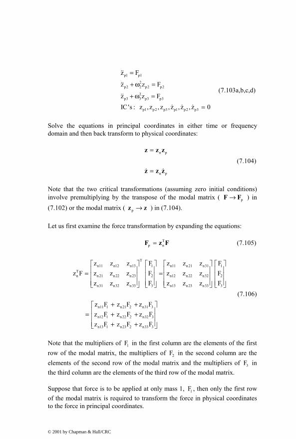
(7.103a,b,c,d)

Solve the equations in principal coordinates in either time or frequency domain and then back transform to physical coordinates:

n p

n p

=

=

z z z

z z z& &

(7.104)

Note that the two critical transformations (assuming zero initial conditions) involve premultiplying by the transpose of the modal matrix ( p→F F ) in (7.102) or the modal matrix ( p →z z ) in (7.104).

Let us first examine the force transformation by expanding the equations:

Tp n=F z F (7.105)

Tn11 n12 n13 1 n11 n21 n31 1

Tn n21 n22 n23 2 n12 n22 n32 2

n31 n32 n33 3 n13 n23 n33 3

n11 1 n21 2 n31 3

n12 1 n22 2 n32 3

n13 1 n23 2 n33 3

z z z F z z z Fz F z z z F z z z F

z z z F z z z F

z F z F z Fz F z F z Fz F z F z F

= =

+ + = + + + +

(7.106)

Note that the multipliers of 1F in the first column are the elements of the first row of the modal matrix, the multipliers of 2F in the second column are the elements of the second row of the modal matrix and the multipliers of 3F in the third column are the elements of the third row of the modal matrix.

Suppose that force is to be applied at only mass 1, 1F , then only the first row of the modal matrix is required to transform the force in physical coordinates to the force in principal coordinates.


Now let us examine the displacement transformation by expanding the equations:

n p=z z z (7.107)

1 n11 n12 n13 p1 n11 p1 n12 p2 n13 p3

2 n p n21 n22 n23 p2 n21 p1 n22 p2 n23 p3

3 n31 n32 n33 p3 n31 p1 n32 p2 n33 p3

z z z z z z z z z z zz z z z z z z z z z zz z z z z z z z z z z

+ + = = = = + + + +

z z z

(7.108)

Note that the coefficients of the principal displacements in the first row above are the elements of the first row of the modal matrix. Similarly, coefficients of the second and third rows are the elements of the second and third rows of the modal matrix.

Suppose that the only physical displacement we are interested in is that of mass 2, 2z , then only the second row of the modal matrix is required to transform the three displacements p1 p2 p3z , z , z in principal coordinates to 2z . This leads to the following conclusion about reducing the size of the model:

Only the rows of the modal matrix that correspond to degrees of freedom to which forces are applied and/or for which displacements are desired are required to complete the model.

For this tdof model, reducing the size of the problem is not required; however, we will see later that a realistic finite element model, with hundreds of thousands of degrees of freedom, presents an entirely different problem. Having the ability to reduce the problem size is critical in order to use the detailed results of a complicated finite element model to provide accurate results in a lower order MATLAB model.

7.10 Damping in Systems with Principal Modes

7.10.1 Overview

Damping in complex built-up mechanical systems is impossible to predict with the present state of the art. We will discuss in this section the conditions which determine if a damping matrix can be diagonalized, and the criterion to enable the damped equations to be diagonalized. In general, an arbitrary damping matrix cannot be diagonalized by the undamped eigenvectors, as the


mass and stiffness matrices can. This leads to using what is called “proportional damping” in most finite element simulations.

If a mechanical system is designed with a specific viscous damping element, for example a dashpot, that dominates the small amount of inherent structural damping present, then that element can be added to the system as a viscous damper. The resulting system is linear, but probably does not exhibit normal modes as discussed in Section 7.2.2. In general this leads to the inability to diagonalize and uncouple the equations of motion, requiring a state space solution of the original, coupled equations of motion.

Viscoelastic damping treatments (damping elastomers) have been used for years in disk drives, most typically as constrained layer dampers on the thin sheet metal suspensions which support the read/write head. The effect of this viscoelastic damping can be approximated at a specific temperature and frequency as proportional damping by using the “modal strain energy” technique in association with a finite element structural model (Johnson 1982).

Ignoring specific viscous, coulomb, and viscoelastic damping elements, damping in typical structures arises from hysteresis losses in the materials as they are strained, in some cases from viscous losses due to structure/fluid interaction but more importantly from relative motion at the interfaces and boundaries where different parts are attached or grounded. Unless a specific damping element is used in a structural design, most structures have damping which varies from mode to mode and will be in the range of 0.05% to 2% of critical damping.

The modes in this chapter are all “real” or “normal” modes as defined earlier. Once again, having normal modes means that at certain frequencies all points in the system will vibrate at the same frequency and in phase, i.e., all points in the system will reach their minimum and maximum displacements at the same point in time. Chapter 5 discussed “complex” modes, modes in which all points in the system do not reach their minimum and maximum displacements at the same point in time.

7.10.2 Conditions Necessary for Existence of Principal Modes in Damped System

With a conservative (no damping) system, normal modes of vibration will exist. In order to have normal modes in a damped system, the mode shapes must be the same as for the undamped case, and the various parts of the system must pass through their minimum and maximum positions at the same instant in time, expressed as:


( ) thi mi i it for the i modecos= ω + φz z (7.109)

A sufficient condition for the existence of damped normal modes is that the damping matrix be a linear combination of the mass and stiffness matrices. We know that m and k are diagonalized by operating on them with the modal matrix. When c is a linear combination of m and k , then the damping matrix c is also uncoupled (diagonalized) by the same pre- and postmultiplication operations by the modal matrix as with the m and k matrices (Weaver 1990, Craig 1981).

The damped equations of motion then become:

+ + =mz cz kz F&& & , (7.110)

where the damping matrix is a linear combination of and m k :

a b= +c m k (7.111)

Tp n n=c z cz , (7.112)

and where nz is the normalized (with respect to mass) modal matrix.

Writing out the complete equation:

+ + =mz cz kz F&& & (7.113)

{ {{ {{ {− − −+ + =T 1 T 1 T 1 T

n n n n n n n n n n

p p p p p p

z mz z z z cz z z z kz z z z Fz c z k z FI&& &

123&& &

(7.114)

Looking at the c to pc conversion where a b= +c m k :

a b= +c m k (7.115)

a b= +T T Tn n n n n nz cz z mz z kz

pa b= +I k , (7.116)

where pk is a diagonal matrix whose elements are the squares of the eigenvalues.


The equation for the ith mode is:

( )2 2pi i pi i pi piz a b z z F+ + ω + ω =&& & (7.117)

Rewriting, defining pc , the ( )2ia b+ ω term, using notation:

2pi i i ic a b 2= + ω = ζ ω (7.118)

Where iζ is the percentage of critical damping for the ith mode, defined as:

i i ii 2

cr pi pii pi i

c c cc 2 k m 2m

ζ = = =

ω (7.119)

Then:

2i

ii

a b2+ ωζ =

ω (7.120)

Rewriting the equation in principal coordinates:

2pi i i pi i pi piz 2 z z F+ ζ ω + ω =&& & (7.121)

This type of damping is known as proportional damping, where the damping for each mode (they can all be different) is proportional to the critical damping for that mode. Since the damping is also proportional to velocity, it is of a viscous nature. If the same damping value is used for all modes, it will be referred to as “uniform” damping. Damping in which the damping value for each mode can be set individually will be referred to as “non-uniform” damping.

7.10.3 Different Types of Damping

7.10.3.1 Simple Proportional Damping

Viscous damping in each mode is taken to be an arbitrary percentage, ζ , of critical damping:


2pi i pi i pi pi

12

p p p p p p

z 2 z z F

2

+ ζω + ω =

+ ζ + = z k z k z F

&& &

&& & (7.122)

This is analogous to the familiar notation used for a single degree of freedom system:

mz cz kz Fc k Fz z zm m m

+ + =

+ + =

&& &

&& & (7.123)

Define critical damping crc 2 km= and define the term multiplying velocity to be:

n

cr

c 2m

c k2c m

2c k2 km mcm

= ζω

=

=

=

(7.124)

Rewriting:

2n n

Fz 2 z zm

+ ζω + ω =&& & (7.125)

7.10.3.2 Proportional to Stiffness Matrix – “Relative” Damping

Recognizing that the higher modes of vibration damp out quickly, “relative” damping yields damping in proportion to frequencies in normal modes, basically letting the “a” term for iζ go to zero:

2i i

ii

a b b2 2

a 0

+ ω ωζ = =ω

=

7.126)

If a value of 1ζ , for the first mode, is assumed, a value can be defined for “b”:


1

1

2b ζ=ω

, (7.127)

and the value for any other mode i is:

ii 1

1

ωζ = ζω

(7.128)

7.10.3.3 Proportional to Mass Matrix – “Absolute” Damping

Absolute damping is based on making “b” equal to zero, in which case the percentage of critical damping is inversely proportional to the natural frequency of each mode. This will give decreasing damping for modes as their frequencies increase.

2i

ii i

a b a2 2

b 0

+ ωζ = =ω ω

=

(7.129)

If a value of 1ζ , for the first mode, is assumed, a value can be defined for “a”:

1 1a 2= ζ ω , (7.130)

and the value for any other mode i is:

1 1i

i

ω ζζ =ω

(7.131)


7.10.4 Defining Damping Matrix When Proportional Damping is Assumed

Figure 7.6: Two degree of freedom for damping example.

An interesting question to ask is what the elements of the damping matrix should be in the two degree of freedom (2dof) problem shown in Figure 7.6 in order to be able to diagonalize the equations of motion. We will use the eigenvectors from the undamped case to normalize the damping matrix. Then we will solve for the specific values of the individual dampers which will allow the diagonalization. We will see how non-intuitive the values of

1 2 3c , c and c are in order to be able to diagonalize. (See Craig [1981] for a general expression to calculate the physical damping matrix when given proportional damping values, the original mass matrix, the diagonalized mass matrix and the eigenvalues and eigenvectors.)

7.10.4.1 Solving for Damping Values

Starting with the undamped eigenvalues and eigenvectors:

1 2 2

2 2 3

m n p

c c cm 0 2k kc c c0 m k 2k

k 01 1 1 11 m1 1 1 1 3k2m 0

m

+ −− = = = − +−

= = = − −

m k c

z z k

(7.132)

Solve for the diagonalized damping matrix, assuming proportional damping, and knowing that the diagonalized stiffness matrix elements are squares of the eigenvalues:

c2

m m

k kz1 z2F1 F2

c1

k

c3


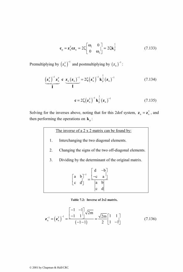
11T 2

p n n p2

02 2

0ω

= = ζ = ζ ω c z cz k (7.133)

Premultiplying by ( ) 1Tnz

− and postmultiplying by ( ) 1

nz − :

( ) ( ) ( ) ( )1

1 11 1T T T 2n n n n n p n2

− −− −= ζz z c z z z k z

II1424314243

(7.134)

( ) ( )1

1 1T 2n p n2

− −= ζc z k z (7.135)

Solving for the inverses above, noting that for this 2dof system, Tn n=z z , and

then performing the operations on pk :

The inverse of a 2 x 2 matrix can be found by:

1. Interchanging the two diagonal elements.

2. Changing the signs of the two off-diagonal elements.

3. Dividing by the determinant of the original matrix.

1

d ba b c a

a bc dc d

−−

− =

Table 7.2: Inverse of 2x2 matrix.

( ) ( )11 T

n n

1 12m

1 11 1 2m1 11 1 2

−−

− − − = = = −− −

z z (7.136)


11 2

n p

1 01 12m k1 12 m 0 3

1 32k2 1 3

− = −

=

−

z k

(7.137)

11 12

n p n

1 3 1 12k 2m1 12 21 3

1 3 1 32 km4 1 3 1 3

− −

= −−

+ −=

− +

z k z

(7.138)

1 3 1 3km22 1 3 1 3

1 3 1 3km

1 3 1 3

+ −= ζ

− +

+ −= ζ

− +

c

(7.139)

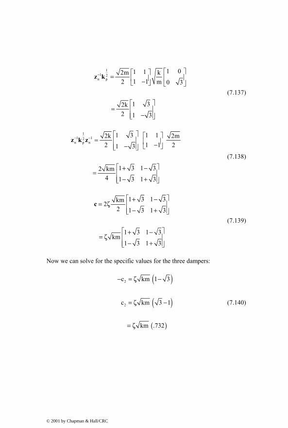
Now we can solve for the specific values for the three dampers:

( )

( )

( )

2

2

c km 1 3

c km 3 1

km .732

− = ζ −

= ζ −

= ζ

(7.140)


( )

( )

( ) ( )

( )

1 2 2 3

1 3 2

c c c c km 1 3

c c km 1 3 c

km 1 3 3 1

km 2

2 km

+ = + = ζ +

= = ζ + −

= ζ + − −

= ζ

= ζ

(7.141)

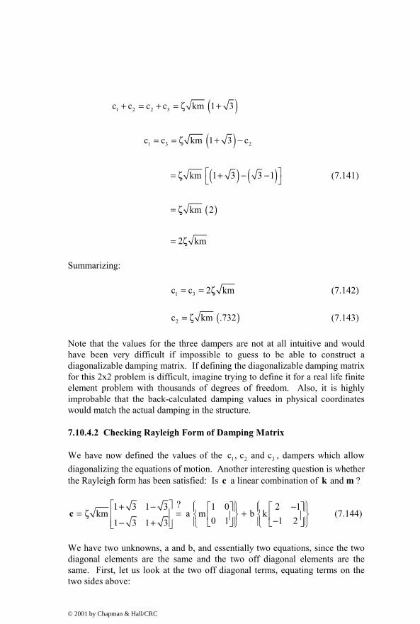
Summarizing:

1 3c c 2 km= = ζ (7.142)

( )2c km .732= ζ (7.143)

Note that the values for the three dampers are not at all intuitive and would have been very difficult if impossible to guess to be able to construct a diagonalizable damping matrix. If defining the diagonalizable damping matrix for this 2x2 problem is difficult, imagine trying to define it for a real life finite element problem with thousands of degrees of freedom. Also, it is highly improbable that the back-calculated damping values in physical coordinates would match the actual damping in the structure.

7.10.4.2 Checking Rayleigh Form of Damping Matrix

We have now defined the values of the 1 2 3c , c and c , dampers which allow diagonalizing the equations of motion. Another interesting question is whether the Rayleigh form has been satisfied: Is c a linear combination of and k m ?

?1 3 1 3 1 0 2 1km a m b k

0 1 1 21 3 1 3

+ − − = ζ = + − − + c (7.144)

We have two unknowns, a and b, and essentially two equations, since the two diagonal elements are the same and the two off diagonal elements are the same. First, let us look at the two off diagonal terms, equating terms on the two sides above:


( ) ( ) ( )

( ) ( )

km 1 3 am 0 bk 1

3 1 mb km 3 1k k

ζ − = + −

−= ζ = ζ −

(7.145)

Now, equating the diagonal terms:

( )

( )

( )

km 1 3 am 2bk

mam 2 3 1 kk

am 2 mk 3 1

ζ + = +

= + ζ −

= + ζ −

(7.146)

( ) ( )am km 1 3 2 mk 3 1

km 1 3 2 3 2

km 3 3

= ζ + − ζ −

= ζ + − +

= ξ −

(7.147)

ka 3 3m = ζ − (7.148)

Checking the two values for a and b by substituting back into (7.146).


( )

( ) ( )

( )( )

1 3 1 3 1 0kkm m 3 30 1m1 3 1 3

2 1m k 3 11 2k

3 3 0 2 3 2 3 1km

3 1 2 3 20 3 3

1 3 1 3km

1 3 1 3

+ − ζ = ζ − − + −

+ ζ − −

− − − + = ζ + − + − −

+ −= ζ

− +

(7.149)

So c is a linear combination of and k m and the Rayleigh criterion holds.

Problems

Note: All the problems refer to the two dof system shown in Figure P2.2.

P7.1 Set 1 2m m m 1= = = , 1 2k k k 1= = = and solve for the eigenvalues and eigenvectors of the undamped system. Normalize the eigenvectors to unity, write out the modal matrix and hand plot the mode shapes

P7.2 Normalize the eigenvectors in P7.1 with respect to mass and diagonalize the mass and stiffness matrices. Identify the terms in the normalized mass and stiffness matrices. Write the homogeneous equations of motion in physical and principal coordinates.

P7.3 Convert the following step forcing function and initial conditions in physical coordinates to principal coordinates:

a) 1 2F 1, F 3= = −

b) 1 1 2 2z 0, z 2, z 1, z 2= = − = − =& &

P7.4 Using the results of P7.2 and P7.3, write the complete equations of motion in physical and principal coordinates assuming proportional damping.


chapter 07: modal analysis - pudn.comsummarizing the modal analysis method of analyzing ... sdof...

Documents