chapter 05 - influence grid resolution

5.1

5 Influence of Model Grid Resolution on Tropospheric Ozone Levels: the Necessity of High Resolution for Photochemical Modeling in Very Complex Terrains

Published as Jiménez, P., Jorba, O., Parra, R., Baldasano, J.M., 2005. Influence of high model grid resolution on photochemical modeling in very complex terrains. International Journal of Environment and Pollution (In Press).

5.1 Introduction The northeastern Iberian Peninsula (NEIP) has a complex topography with a large coast to the Mediterranean Sea. The complex configuration of the zone comes conditioned by the presence of the Pyrenees mountain range (with altitudes over 3000m), the influence of the Mediterranean Sea and the large valley canalization of Ebro River. That produces a sharp gradient in its characteristics. This sort of terrain induces an extremely complicated structure of the flow because of the development of large and local mesoscale phenomena that interact with synoptic flows. The characteristics of the breezes have important effects in the dispersion of the pollutants emitted. In addition, the flow can be even more complex because of the non-homogeneity of the terrain, the land-use and the types of vegetation. In these situations, the structure of the flow is extremely complicated because of the superposition of circulations of different scale. Hence, the study of photochemical pollution in complex terrains demands a high horizontal spatial resolution. The average volume defined by the model’s horizontal grid spacing must be sufficiently small to allow the air quality to be reproduced accurately. The large averaging volumes used by regional models are feared to lead to unacceptable errors for many species that are formed via nonlinear chemical reactions (e.g. ozone and its precursors), particularly in areas with significant chemical gradients, such as cities (Russell and Dennis, 2000). On the other hand, small-scale topographical features captured by small grid spacing in the model can result in numerical instabilities that contaminate predictions. For all these reasons, and since computational requirements increase markedly with the inverse of the grid spacing (for a given domain), the grid size becomes an important design decision. Increasing spatial resolution of a meteorological model allows one to include more mesoscale motions in its numerical solution (Pielke and Uliasz, 1998). McQueen et al. (1995) performed a sensitivity analysis on the influence of grid size when applying an operational mesoscale numerical weather prediction model. The study showed the importance of using high-resolution

Air quality modeling in very complex terrains: ozone dynamics in the northeastern Iberian Peninsula

5.2

grids when the model is applied to a complex terrain. Horizontal resolutions up to 1-km should be considered when simulating vertical motion associated with see breezes (Lyons et al., 1995). Jang et al. (1995a; 1995b) studied the sensitivity of ozone to the horizontal grid resolution of air quality models, concluding that a coarser grid size tends to underestimate the maximum ozone levels and to overestimate minimum values, since the grid resolution highly influences the formation and loss processes of ozone, specially photochemical and vertical transport phenomena. The best agreement between the predictions and the observations was attained with horizontal resolutions of 2.5 km. Byun and Dennis (1995) revealed that a 15-layer vertical resolution with RADM model better represents the surface dry-deposition processes and surface concentration of photochemical pollutants than a 6-layer resolution, being the latter inadequate in estimating the pollutants under stable atmospheric conditions; the necessity for a high vertical resolution comes conditioned by the short scale of vertical mixing of certain gas reactions. Thunis (2001) indicated that ozone concentration fields obtained with similar meteorology and emissions but with different horizontal spatial resolutions in the Milan area produced similar O3 surface field patterns, but significant differences were obtained for peak concentrations (20%) between a 10- and a 50-km grid, whereas the 4- and 10-km simulation gave similar results. In the case study of the northeastern Iberian Peninsula, the work of Soriano et al. (1997) showed that a 2-km grid resolution described correctly the forcing caused by the topography in the Barcelona Geographical Area, with no improvement in modeling results when increasing the horizontal resolution to 1 or 0.5 km. Salvador et al. (1999) analyzed the improvement of the results when modifying the grid resolution for a domain covering the eastern Iberian Peninsula. Authors stated the enhancement in the description of meteorological phenomena in a small scale when working with resolutions of 2 km or finer. This study covers grid resolution of 6, 4, 2 and 1.5 km, obtaining significant differences in the performance of simulation results. Nevertheless, simulations with a 1.5-km grid entail an execution time 20 times higher than the corresponding 2-km simulation. Consequently, the precise definition of the grid resolution is an important decision when applying an air quality model. In order to illustrate the influence of grid size on ground-level O3, this work encloses a detailed study of the observable differences in values, location and temporal behavior of tropospheric O3 in the northeastern Iberian Peninsula when applying a three-dimensional air quality model with different horizontal (8, 4 and 2-km) resolutions. It is also assessed how much of the systematic model bias can be explained by changing the vertical grid resolution, when 6 or 16 layers in sigma-coordinates are used in the troposphere.

5.2 Methods Several simulations with the three-dimensional air quality model MM5-EMICAT2000-CMAQ (defined in Section 2.2) are carried out using different grid resolutions: 8-km, 4-km and 2-km. The

Chapter 5. Influence of model grid resolution on tropospheric ozone levels

5.3

domain of study covers the northeastern Iberian Peninsula (a squared area of 272 x 272 km2). The model is configured with both 6 and 16 vertical layers to cover the troposphere, with special emphasis in the low troposphere (4,000 meters). The first layer considers a thickness of 150 m (for the 6 vertical layers case) and 36 m (for the 16 vertical layers case). Layers of both the 6-layer simulation and the 16-layer simulation were obtained by collapsing the 29 layers of the MM5 simulation. The episode selected for studying the influence of the horizontal and vertical model resolution on the concentrations of gas-phase photochemical pollutants was 13-16 August, 2000, which is representative of a photochemical pollution episode, which covered the whole Western Mediterranean Basin (see Section 2.1 for further details). For the assessment of the performance of MM5 meteorological model when considering different resolutions, simulation results were compared with surface and aloft wind measurements. Validation data of 52 surface stations located across the domain, and a radiosonde launched in Barcelona (in the center of the domain in the coast) were used. Ground-level O3 simulation results were compared with the measurements from 48 surface stations in the NEIP (Catalonia, Spain), located in urban, industrial and background areas. Hourly measures of ozone were utilized to indicate the performance of the chemical transport model results when employing different horizontal and vertical resolutions. The analysis of the results consists in a statistical comparison (both discrete and categorical parameters) between the first-layer simulations results and the values measured in the air quality stations of the domain under study. Both meteorological and air quality data were provided by the Environmental Department of the Catalonia Government.

5.3 Influence of Model Resolution on Wind Fields Grid size is influenced primarily by local topography (Salvador et al., 1999). Topographical variations can have an important effect on mesoscale atmospheric flow and, therefore, although topography is not the only driving mechanism that contributes to the dispersion of pollutants in the given domain, it plays a major role and should be well resolved in modeling exercises. The topography of the domain of study is organized from three structural units forming a fan-shape formation with the vertex in the Empordà: (1) Pyrenees, forming a barrier at the north of the region and expanding from east to west, constitute the first great unity; (2) the Central Depression stretches all interior zones, and (3) the Mediterranean System, formed by the joint of mountain ranges and depressions parallel to the coast. Figure 5.1 represents the topographic map of the domain at an 8-km, 4-km and 2-km resolution. There are several significant differences between the coarse and fine topography. Nevertheless, we must bear in mind that smoothing is sometimes positive to avoid the strong topographical gradients that may not be properly resolved by the models (McQueen et al., 1995).


5.4

Figure 5.1. Surface wind field in the northeastern Iberian Peninsula (left) and vertical profile Mediterranean Sea-Barcelona-Pyrenees (right) for 14 August, 2000, at 1200UTC. 8-km grid (up), 4-km (center) and 2-km grid (down).


5.5

Results depict that important mesoscale phenomena within the region do not develop in the domain of study if the horizontal resolution is coarser than 4-km. Under low synoptic forcings, mountain winds develop because of the very complex topography of the region, while the difference of temperature between the sea and the land enhances the development of sea-land breezes. Clear differences are observed in the wind direction, especially over the sea (Figure 5.1). The daily cycle of these flows constitutes an important part of the mechanism that drives the transport of air pollutants within the region. Results show how the see breeze development is well captured by all simulations; even though, particular canalizations of the flow are only appreciable at 4- and 2-km resolutions. With lower resolutions, wind fields present a too smoothed structure. More differences appear with mountain-winds, which are not developed at 8-km. Only with a fine high resolution, the meteorological model is able to reproduce the mountain-wind system; coarser resolution simulations do not manage to describe the complexity observed in the Pyrenees, whose influence is more stressed when incrementing resolution to 2-km. The coastal mountain range orientation (SW-NE) favors a rapid solar heating of slopes and an early onset of the sea breeze, aided by the upslope winds. Because of the orientation of the mountain ranges, thermal effects intensify the sea breeze. The vertical structure of the flows is also influenced by the best representation of the topography when working with high horizontal resolution. An enhancement of vertical motions is observed, and the vertical structure of the see-breeze is improved, and several orographic injections appear when increasing the resolution. Nighttime regime differs substantially in both simulations, with down-slope and down-valley winds in the Pyrenees valleys (Cerdanya) that are observable in the finest grid but are not described by the 8-km or 4-km grid. Table 5.1 shows the root mean square error (RMSE) of wind speed at 10 m, for the lower, middle and upper troposphere and RMSE of wind direction at 10 m for the different horizontal resolutions. The general behavior of the model shows a tendency to overestimate nocturnal surface winds and to underestimate the diurnal flow. A clear improvement is produced with 2-km simulation during the central part of the day. The complex structure of the see-breeze described by the 2-km simulation, and the development of up-slope winds appear to agree in a higher grade with surface measurements. Statistics show how the model presents a better behavior within the boundary layer, and major disagreement with the radiosonde appears over 1000 m agl. At night, 8- and 4-km presents better results aloft, while at noon the high horizontal resolution simulation obtains the best statistics.


5.6

Table 5.1. RMSE statistic of wind speed, and wind direction for 2-, 4-, 8-km simulations at 0000, 1200, 2400UTC (surface values evaluated with 52 surface stations, aloft values evaluated with a radiosonde).

RMSE Wind speed (m/s) 0000UTC 1200UTC 2400UTC 2 km 4 km 8 km 2 km 4 km 8 km 2 km 4 km 8 km Surface 10 m 1.71 1.85 1.76 2.04 2.34 2.41 2.00 2.17 2.22 Radio. <1000 m 0.84 1.02 1.04 1.04 1.08 1.34 1.31 0.86 0.86 1000-5000 m 5.03 3.95 3.66 1.55 2.40 2.16 3.70 2.59 2.27 5000-10000 m 8.45 8.92 8.62 5.15 6.22 6.3 3.94 5.29 5.16

RMSE Wind direction (º) 0000UTC 1200UTC 2400UTC 2 km 4 km 8 km 2 km 4 km 8 km 2 km 4 km 8 km Surface 10 m 95.95 91.33 92.10 44.74 58.17 55.25 89.40 98.59 94.69

5.4 Importance of Resolution on Emissions The main emissions sources in the northeastern Iberian Peninsula are located on the coast. Total emissions of ozone precursors during 14 August, 2000 were 236 t d-1 for NOx and 172 t d-1 for VOCs. Importance of biogenic emissions is high in the area, since this source represents 34% of VOCs emissions in the northeastern Iberian Peninsula during this summer episode and is an important source of reactive compounds such as aldehydes and isoprene (Parra et al., 2004). Road traffic accounts for a 58% of NOx emissions and 36% of VOCs in the domain, especially olefins and aromatic compounds (Parra and Baldasano, 2004). Most important emitters are found along the road-axis parallel to the coast and Barcelona Geographical Area. Industrial emissions are principally located in the industrial area of Alcover, downwind the city of Tarragona, one of the most important industrial centers in Spain; and represent 39% of NOx emissions and 17% of VOCs, meanwhile the use of residential and domestic solvent use provides the 13% of VOCs emissions in the area (Parra, 2004). The peculiar topography of the zone is the principal driving mechanism that contributes to the dispersion of pollutants emitted in the given domain. The generation of boundary conditions for the domain of the northeastern Iberian Peninsula requires of photochemical inputs from a coarser domain; therefore, these conditions were derived from a one-way nested simulation as indicated in Chapter 4. Cells from the European EMEP mesh have a resolution of 50 km in polar coordinates; meanwhile EMICAT2000 provides a horizontal resolution of 1 km. Table 5.2 shows a comparative summary of annual emissions of primary air pollutants provided by EMEP inventory and EMICAT2000 for the year 2000. The annual EMICAT2000 vegetation emission (46.9 kt of NMVOC) is 52% lower than the estimation by EMEP (sector 11) in an equivalent domain (Figure 5.2). A summary of vegetation emissions at European level is included in EEA (2003). This information was taken from Simpson et al. (1995) and Guenther et al. (1995). For Spain the total annual estimation is 657 kt yr-1 (21% of isoprene, 38% of monoterpenes and 41% of OVOCs).


5.7

Table 5.2. Comparative summary of sectorial annual emissions from EMICAT2000 with EMEP European Inventory (kt yr-1) for the domain of the northeastern Iberian Peninsula.

Air pollutant EMEP 2000 (50x50 km2 cells)

EMICAT2000 (1x1 km2 cells)

Vegetation Isoprene - 5.9

Monoterpenes - 24.7 Other NMVOCs - 16.3

Total 88.8 46.9 On-road traffic

NOx 84.8 62.4 CO 274.2 259.0

NMVOCs 58.0 50.5 SO2 2.7 1.3

CO2 eq. - 8302 Power generation

NOx 11.5 15.0 CO 1.3 2.1

NMVOCs 0.4 0.7 SO2 38.5 28.5

CO2 eq. - 5698 Industrial activities (except power generation) NOx 30.9 26.1 CO 23.5 5.4

NMVOCs 21.8 22.0 SO2 47.2 32.7

CO2 eq. - 14663

Figure 5.2. Comparison of EMICAT2000 (left) and EMEP (right) biogenic emissions estimates for the northeastern Iberian Peninsula during year 2000.

NMVOCs kg km-2 yr-1 NMVOCs t cell-1 yr-1

Total: 46.9 kg yr-1 Total: 88.8 kg yr-1


5.8

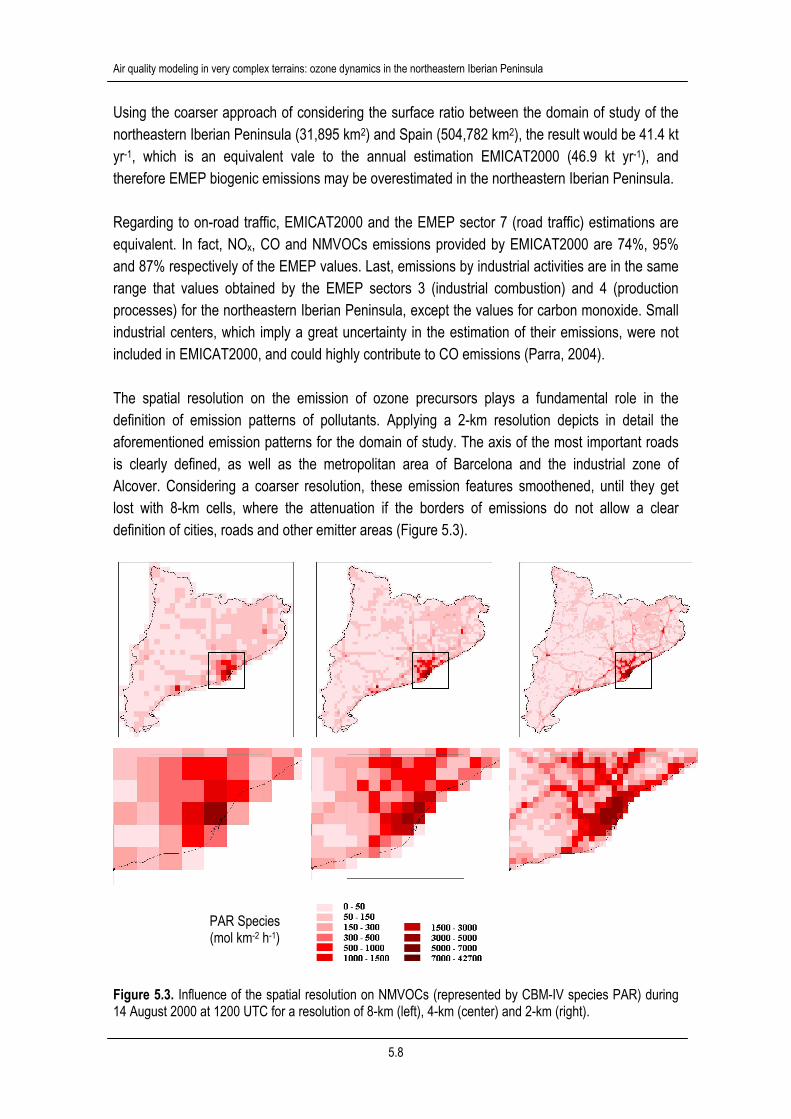
Using the coarser approach of considering the surface ratio between the domain of study of the northeastern Iberian Peninsula (31,895 km2) and Spain (504,782 km2), the result would be 41.4 kt yr-1, which is an equivalent vale to the annual estimation EMICAT2000 (46.9 kt yr-1), and therefore EMEP biogenic emissions may be overestimated in the northeastern Iberian Peninsula. Regarding to on-road traffic, EMICAT2000 and the EMEP sector 7 (road traffic) estimations are equivalent. In fact, NOx, CO and NMVOCs emissions provided by EMICAT2000 are 74%, 95% and 87% respectively of the EMEP values. Last, emissions by industrial activities are in the same range that values obtained by the EMEP sectors 3 (industrial combustion) and 4 (production processes) for the northeastern Iberian Peninsula, except the values for carbon monoxide. Small industrial centers, which imply a great uncertainty in the estimation of their emissions, were not included in EMICAT2000, and could highly contribute to CO emissions (Parra, 2004). The spatial resolution on the emission of ozone precursors plays a fundamental role in the definition of emission patterns of pollutants. Applying a 2-km resolution depicts in detail the aforementioned emission patterns for the domain of study. The axis of the most important roads is clearly defined, as well as the metropolitan area of Barcelona and the industrial zone of Alcover. Considering a coarser resolution, these emission features smoothened, until they get lost with 8-km cells, where the attenuation if the borders of emissions do not allow a clear definition of cities, roads and other emitter areas (Figure 5.3).

Figure 5.3. Influence of the spatial resolution on NMVOCs (represented by CBM-IV species PAR) during 14 August 2000 at 1200 UTC for a resolution of 8-km (left), 4-km (center) and 2-km (right).

PAR Species (mol km-2 h-1)


5.9

5.5 Influence of Model Resolution on Ground-Level Ozone The US Environmental Protection Agency has developed guidelines (USEPA, 1991) drawn from Tesche et al. (1990) for a minimum set of statistical measures to be used for these evaluations where monitoring data are sufficiently dense. Those statistical figures are: mean normalized bias error (MNBE), mean normalized gross error for concentrations above a prescribed threshold (MNGE), and unpaired peak prediction accuracy (UPA). The values for the MNBE and UPA can be either positive or negative. Observation/prediction pairs were often excluded from the analysis if the observed concentration was below a certain cut-off; the cut-off levels varied from study to study but often a level of 120 µg m-3 is used (Hogrefe et al., 2001), which is the criterion applied in this work. Categorical statistics, as derived from Kang et al. (2003), have also been used to evaluate the different vertical and horizontal resolution, including parameters as the model accuracy (A), bias (B), probability of detection (POD), false alarm rates (FAR) and critical success index (CSI). These criteria based also upon a 120 µg m-3 threshold. Table 5.3 collects the results of the statistical analysis; although there is no objective criterion set forth for a satisfactory model performance, suggested values of ±10–15% for MNBE, ±15–20% for the UPA and +30–35% for the MNGE to be met by modeling simulations of O3 have been considered for regulatory applications, as discussed by Russell and Dennis (2000). We should bear in mind, however, that a surface measurement represents a value only at a given horizontal location and height, while the concentration predicted by the model represents a volume-averaged value. Table 5.3. Summary results for evaluation of ozone concentrations with different horizontal and vertical resolutions.

Max Obs (µg m-3) 189 Max Sim (µg m-3) 207 188 131 143 137 144

Discrete Evaluation 2km/6layers 2km/16layers 4km/6layers 4km/16layers 8km/6layers 8km/16layers MNBE (%) -2.02 -11.38 -9.53 -16.92 -12.86 -13.12 MNGE (%) 19.72 20.89 17.42 21.61 19.27 21.01 UPA (%) 17.08 -0.76 -26.07 -19.24 -22.53 -18.49

Categorical Evaluation 2km/6layers 2km/16layers 4km/6layers 4km/16layers 8km/6layers 8km/16layers A (%) 90.9 91.6 91.5 92.4 91.6 91.7 CSI (%) 19.0 12.5 3.2 8.9 3.2 10.0 POD (%) 26.4 14.9 3.4 9.2 3.4 11.5 B (%) 0.7 0.3 0.1 0.1 0.1 0.3 FAR (%) 59.6 56.7 72.7 27.3 70.0 56.5


5.10

Progressively increasing grid resolution from 8-km to 2-km improves the performance of all statistical parameters. The MNBE is negative for every simulation, ranging from -16.92% for 4km/16layers until -2.02% for 2km/6layers case. The MNGE is similar in all cases studied, being within the aforementioned standards. The UPA does not greatly improve when augmenting the resolution from 8-km to 4-km, but this improvement becomes evident in the 2-km/16layers simulation, yielding values of -0.76% for the highest vertical and horizontal resolution. Respect to categorical forecasting, statistical parameters indicate that the accuracy (percent of forecasts that correctly predict an exceedance or non-exceedance) is above 90% for every resolution, but yielding the best parameters for the 16-vertical layers resolution respect to the coarser vertical resolution. Since this metric can be greatly influenced by the overwhelming number of non-exceedances, to circumvent this inflation the critical success index and the probability of detection are used. Both parameters perform similarly during the episode, yielding more accurate values when using a 2-km resolution (and thus, when exceedances of the 120 µg m-3 threshold taken as reference are more frequent). The value of bias (B<1 for all simulations) indicates that exceedances are generally underpredicted for every resolution, which corresponds with the value of MNBE obtained for discrete evaluations, but this underprediction is minor for the 2km/6 layers case (0.7) and the 2km/16 layers case (0.3). Last, the fifth categorical parameter, the false alarm rate, indicated the number of times that the model predicted an exceedance that did not occur. This metric is higher for the simulations with inferior vertical resolution (above 70% for the 4km/6 layers and the 8km/6 layers cases), since of the possible influence of the vertical collapse of emissions, that can be high for the sum of precursor species for O3. Nevertheless, values shown here agree with the results found by Kang et al. (2003). In general, the maximum 1-hr concentration of O3 (Figure 5.4) was overestimated by the 2-km resolution (Table 5.3), being underestimated both by the 8-km and the 4-km simulations. The error reduces substantially when incrementing the vertical grid resolution. The explanation for this behavior is that model outputs indicate an average of the cell, diluting the very local effects of photochemical phenomena. Figure 5.4 depicts that an accurate definition of O3 problem in the region is only achieved when observing the 2-km/16layers case. Average values are underestimated by simulations when using both an 8-km, 4-km or 2-km grid size, exhibiting negative bias resolutions. Figure 5.5 depicts the average values of tropospheric O3 in the domain of study for the different horizontal and vertical resolutions. They present similarities in the prediction of the lowest values in the Barcelona Geographical Area and Tarragona. Nevertheless, 8-km and 4-km simulations do not show a good agree with observations in northeastern area of the domain, and therefore a 2-


5.11

km resolution must be used. The depletion of O3 during the evening and night in Barcelona and the industrial area of Tarragona, and high average background values of ozone in the Pyrenees are only properly observed with resolutions of 4-km and finer, and are better captured with 16 vertical layers.

Figure 5.4. 1-hr maximum ozone levels (µg m-3) in the simulation domain for an 8-km (up), 4-km (center) and 2-km (down) horizontal resolution with 6 (left) and 16 (right) vertical layers for the episode of 13-16 August, 2000.

µg m-3


5.12

Figure 5.5. Average daily ozone levels (µg m-3) in the simulation domain for an 8-km (up), 4-km (center) and 2-km (down) horizontal resolution with 6 (left) and 16 (right) vertical layers for the episode of 13-16 August, 2000. The effects of grid resolution on the chemistry of O3 and NOx are far more important than the chemistry of VOCs (Jang et al., 1995b). The predicted first layer O3 and NOx concentrations by 6- and 16-layer vertical resolutions are distinctively different for the whole domain. Ozone

µg m-3


5.13

predictions from the 6-layer case show slightly higher values than those from the 16-layer model, meanwhile NOx concentrations are significantly higher in the case of 16-layer vertical resolution (Figure 5.6).

0

10

20

30

40

50

60

70

80

90

100

0 1 2 3 4 5 6 7 8 9 10 11 12 13 14 15 16 17 18 19 20 21 22 23

Time (UTC)

O3 A

vera

ge C

once

ntra

tion

( µg

m-3

)

6 layers 16 layers

0

10

20

30

40

50

60

0 1 2 3 4 5 6 7 8 9 10 11 12 13 14 15 16 17 18 19 20 21 22 23

Time (UTC)

NO

x Ave

rage

Con

cent

ratio

n ( µ

g m

-3)

6 layers 16 layers

Figure 5.6. Average daily variation of ozone (up) and nitrogen oxides (down) for 6 and 16 vertical layers simulations in the domain of study, expressed in µg m-3, for the episode of 13-16 August, 2000.


5.14

This can be explained by the fact that the VOCs and NOx emissions injected into the 6-layer model are diluted in a deeper layer compared to the same injected into the 16-layer model. Since most of the domain presents a VOCs-limited sensitivity (Jiménez and Baldasano, 2004), increasing NOx concentration in the first layer presents the contrary effect on tropospheric ozone, producing less ozone from the photochemical reaction and lowering ground-level O3 concentrations. As shown in Table 5.4, coarser cell sizes are too large to correctly represent NOx emissions, which have very distinctive grid-scale distributions; the result of photochemical reactions with diluted primary species concentrations does not give a similar dynamic range as observed ozone concentrations. In addition, performance of the model greatly improves when using 16 vertical layers instead of just 6 layers. The 8-km resolution tempers the concentrations of pollutants, yielding most of values in a medium range, not capturing the extreme values (maximum and minimum levels of NOx) that are more truthfully predicted by the finer resolution. We expect that the limited dynamic range in the daily ozone concentrations is related to the over-smoothing of NOx emission rates in the model with coarse horizontal and vertical resolutions. NOx species is more sensitive than ozone to model grid structure since secondary species have more horizontal homogeneity than primary species. Table 5.4. Summary results for evaluation of nitrogen oxides concentrations with different horizontal and vertical resolutions.

Max Obs (µg m-3) 220 Max Sim (µg m-3) 149 247 154 190 80 141 2km/6layers 2km/16layers 4km/6layers 4km/16layers 8km/6layers 8km/16layers MNBE (%) -28.64 9.46 -23.34 -17.77 -52.32 -32.78 MNGE (%) 39.20 31.36 40.76 41.75 39.73 37.78 UPA (%) -32.20 12.36 -30.13 -13.54 -63.86 -36.10

5.6 Conclusions The effect of grid resolution on the results of an air quality model when applied to very complex terrains as the northeastern Iberian Peninsula has been illustrated in this work. Simulation of 13-16 August, 2000, episode was used to depict the impact of grid resolution on photochemical pollution. For the complex domain studied, a clear improvement in the statistics of O3 values has been observed when increasing model resolution from 8-km to 4 and 2-km; and from 6 to 16 vertical layers. MM5 meteorological simulations clearly show that the description of wind fields improves with finer grids. Results are very sensitive to the degree of topographical smoothing in this very complex terrain. The model is unable to reproduce the mountain-wind system with resolutions


5.15

coarser than 4-km. Statistics of the 2-km simulation present the best behavior during the development of the sea breeze, but all three simulations overestimate surface flows during the nocturnal period. Despite EMEP inventory could not be satisfactorily applied to the description of air pollutants dynamics in the northeastern Iberian Peninsula because of its coarse resolution, it becomes essential to consider the emissions from this inventory in order to generate boundary conditions to the domain of the NEIP through nested simulations; however, the very complex area considered in this study demands a finer resolution. As a global amount, estimations from EMEP and EMICAT2000 are comparable and present similar results. Their main difference comes from the estimation of biogenic emissions, since EMICAT2000 utilizes specific emission factors for the area of study. Outputs from the chemical transport model were sensitive to the grid size employed in the simulations, presenting a higher dependence on horizontal grid than on the vertical resolution when simulating O3; nevertheless, high vertical resolution was found to be as important as horizontal resolution to properly simulate other photochemical pollutants such as NOx. Despite in outline the dynamics of photochemical pollutants as ozone and the patterns of its precursors do not change dramatically, some small-scale features appear when using a resolution of 2-km that cannot be captured with coarser horizontal resolutions. Meanwhile having a finer grid is important for addressing ozone processes in urban and industrial areas, rural areas allow larger grids to capture the nonlinearity of the ozone process. If both discrete and categorical statistical parameters are compared with US EPA’s recommended values, a grid resolution of 2-km, both with 6 or 16 vertical layers, is needed when simulating photochemical pollution in the NEIP in order to ensure that results are inside the range of error tolerated. Nevertheless, the model should have enough vertical resolution (16 layers) in order to represent correctly the low-troposphere processes throughout the day.

5.7 References Byun, D.W., Dennis, R., 1995. Design artifacts in Eulerian air quality models: evaluation of the

effects of layer thickness and vertical profile correction on surface ozone concentrations. Atmospheric Environment, 29, 105-126.

EEA, 2003. EMEP/CORINAIR Emission Inventory Guidebook - 3rd edition. September 2003 Update. Technical report No 30. European Environmental Agency, Copenhagen, Denmark.

Guenther, A., Hewitt, C.N., Erickson, D., Fall, R., Geron, C., Graedel, T., Harley, P., Klinger, L., Lerdau, M., McKay, W.A., Pierce, T., Scholes, B., Steinbrecher, R., Tallamraju, R., Taylor, J., Zimmerman, P., 1995. A global model of natural volatile organic compound emissions. Journal of Geophysical Research, 100, 8873–8892.

Hogrefe, C., Rao, S.T., Kasibhatla, P., Hao, W., Sistla, G., Mathur, R., McHenry, J., 2001. Evaluating the performance of regional-scale photochemical modeling systems: Part II – ozone predictions. Atmospheric Environment, 35, 4175-4188.


5.16

Jang, C.J., Jeffries, H.E., Byun, D., Pleim, J.E., 1995a. Sensitivity of ozone to model grid resolution – I. Application of high-resolution regional acid deposition model. Atmospheric Environment, 29, 21, 3085-3100.

Jang, C.J., Jeffries, H.E., Byun, D., Pleim, J.E., 1995b. Sensitivity of ozone to model grid resolution – II. Detailed process analysis for ozone chemistry. Atmospheric Environment, 29, 21, 3101-3114.

Jiménez, P., Baldasano, J.M., 2004. Ozone response to precursor controls: the use of photochemical indicators to assess O3-NOx-VOC sensitivity in the northeastern Iberian Peninsula. Journal of Geophysical Research, 109, D20309, doi: 10.1029/2004JD004985.

Kang, D., Eder, B.K., Schere, K.L., 2003. The evaluation of regional-scale air quality models as part of NOAA’s air quality forecasting pilot program. In: 26th Nato International Technical Meeting on Air Pollution Modeling and its Application, 26-30 May, Istanbul, Turkey, 404-411.

Lyons, W.A., Pielke, R.A., Tremback, C.J., Walko, R.L., Moon, D.A., Keen, C.S., 1995. Modeling the impacts of mesoscale vertical motions upon coastal zone air pollution dispersion. Atmospheric Environment, 29, 283-301.

McQueen, J.T., Draxler, R.R., Rolph, G.D., 1995. Influence of grid size and terrain resolution on wind field predictions from an operational mesoscale model. Journal of Applied Meteorology, 34, 10, 2166-2181.

Parra, R., 2004. Development of the EMICAT2000 model for the estimation of air pollutants emissions in Catalonia and its use in photochemical dispersion models. Ph.D. Dissertation (in Spanish), Polytechnic University of Catalonia (Spain).

Parra R., Baldasano J.M., 2004. Modelling the on-road traffic emissions from Catalonia (Spain) for photochemical air pollution research. Weekday – weekend differences. In: 12th International Conference on Air Pollution (AP'2004), Rhodes (Greece).

Parra, R., Gassó, S., Baldasano, J.M., 2004. Estimating the biogenic emissions of non-methane volatile organic compounds from the North western Mediterranean vegetation of Catalonia, Spain. The Science of the Total Environment, 329, 241-259.

Pielke, R.A., Uliasz, M., 1998. Use of meteorological models as input to regional and mesoscale air quality models – Limitations and strengths. Atmospheric Environment, 32, 8, 1455-1466.

Russell, A., Dennis, R., 2000. NARSTO critical review of photochemical models and modeling. Atmospheric Environment, 34, 2283-2324.

Salvador, R., Calbó, J., Millán, M.M., 1999. Horizontal grid size selection and its influence on mesoscale model simulations. Journal of Applied Meteorology, 38, 1311-1329.

Simpson, D., Guenther, A., Hewitt, C., Steinbrecher, R., 1995. Biogenic emissions in Europe 1. Estimates and uncertainties. Journal of Geophysical Research, 100(D11), 22875 - 22890.

Soriano, C., Baldasano, J.M., Buttler, W.T., 1997. On the application of meteorological models and lidar techniques for air quality studies at a regional scale. In: Air Pollution Modeling and its Application XII, Gryning, S-E. and Chaumeliac, N. (Eds.), Plenum Press, 591-600.

Tesche, T.W., Lurmann, F.L., Roth, P.M., Georgopoulos, P., Seinfeld, J.H., Cass, G., 1990. Improvement of Procedures for Evaluating Photochemical Models. Report to California Air Resources Board for Contract No. A832-103. Alpine Geophysics, LLC, Crested Butte, Colorado.

Thunis, P., 2001. The influence of scale on modeled ground level O3 concentrations. Norwegian Meteorological Institute Research Report no. 57, EMEP/MSC-W Note 2/01. Copenhagen, Denmark, 42 pp.

US EPA, 1991. Guideline for Regulatory Application of the Urban Airshed Model. US EPA Report No. EPA-450/4-91-013. Office of Air and Radiation, Office of Air Quality Planning and Standards, Technical Support Division. Research Triangle Park, North Carolina, US.

chapter 05 - influence grid resolution

Documents