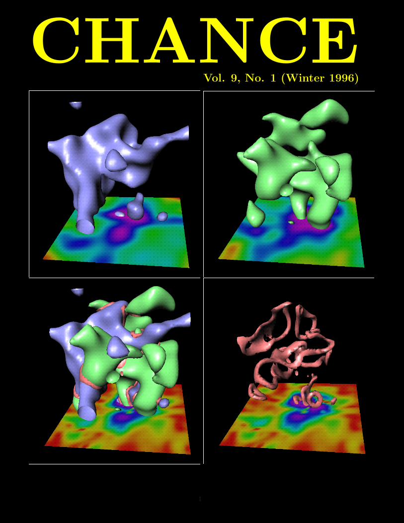
CHANCEVol. 9, No. 1 (Winter 1996)

1

From the human brain to the creation of the universe: Some new discoveries in

statistics and probability, found using tools from topology and geometry, have been

applied to medical imaging and astrophysics.

The Geometry of Random Images

Keith J. Worsley

The geometry in the title is not the geometry of linesand angles but the modern geometry of topology andshape. What has this to do with statistics? Some re-cent work has found some fascinating applications of amixture of geometry, topology, probability, and statis-tics to some very pressing problems in newly emergingareas of medical imaging and astrophysics.

Where is the link? Let us begin with a quick intro-duction to one of the fundamental tools of topology,the Euler characteristic.

Topology: The Euler Characteristic

Named after Leonhard Euler (1707–1783), the mostprolific mathematician of the 18th century, the Eu-ler characteristic itself began with Euler’s observationabout polyhedra.

Recall that a polyhedron is a solid object boundedby plane faces, such as a cube. Euler realized that, ifyou count the faces (F ), edges (E), and vertices (V )of a polyhedron, then V − E + F = 2 no matter howthe polyhedron is constructed.

A cube, for example, has F = 6 faces, E = 12 edgesand V = 8 vertices (see Fig. 1a) so that 8−12+6 = 2.For a solid that consists of P polyhedra, stuck togetheron at least one common face, the slightly more generalformula becomes V − E + F − P = 1.

A little experimentation will convince you that thisnew formula works for all solids (see Fig. 1b)—wellalmost all. If the solid has a hole going right through

it, like a doughnut (see Fig. 1c), then the result nolonger holds. In fact, the result is V −E + F − P = 0for any solid with just one hole.

Too bad! But this does not deter a goodmathematician—far from it—it opens up vast new pos-sibilities! What happens if there are two holes, likea figure 8 (see Fig. 1d)? Then it turns out thatV − E + F − P = −1, and so on; each hole reducesV − E + F − P by 1.

So now suddenly we have a fascinating new tool.We can count the number of holes in a solid using theformula V − E + F − P ; it has the very interestingproperty that no matter how the solid is subdividedinto polyhedra, the value of V −E+F−P is invariant.Thus is born the field of topology: We define the Eulercharacteristic (EC) of a solid as simply

EC = V − E + F − P

for any subdivision of the solid into polyhedra.Thus the EC of a pretzel-shaped solid (Fig. 1e) is

−2: +1 for the solid part (the part you eat), and −3for each of the three holes, giving −2 overall. Havewe covered all possibilities? Not quite—if the solid ishollow, like a tennis ball, then surprisingly enough theEC is 2 (see Fig. 1f).

Think you’ve got it now? How about a solid shapedlike a bicycle inner tube? Answer: The EC is 0, and ifit has a puncture, then the EC is −1.

One more slight generalization, which will prove tobe extremely useful for practical applications: Suppose

27

•

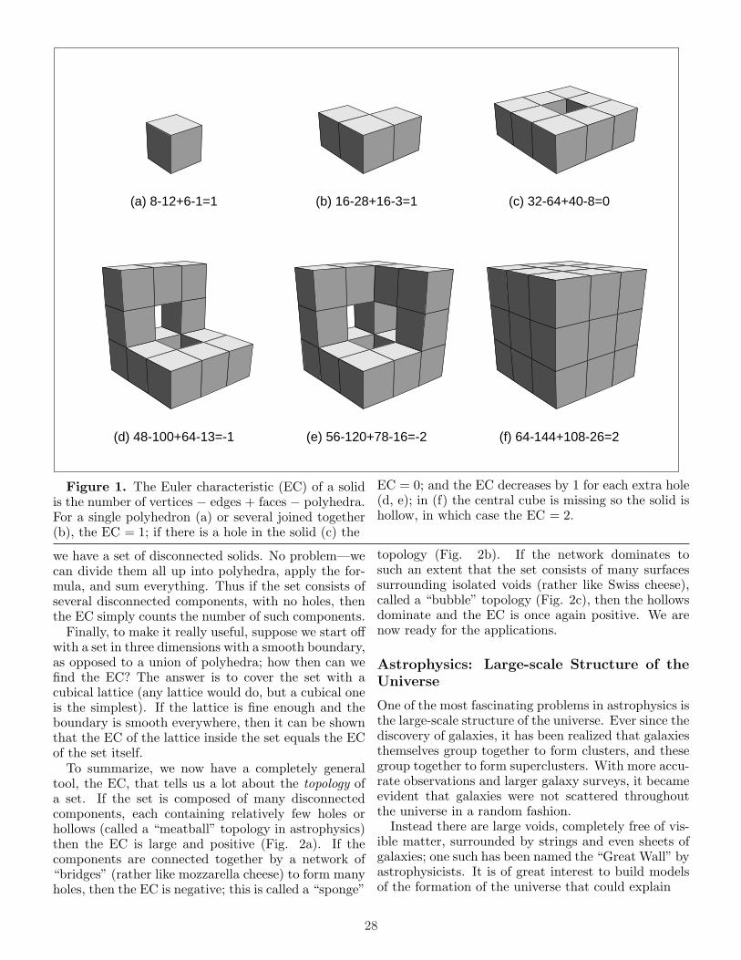
(a) 8-12+6-1=1 (b) 16-28+16-3=1 (c) 32-64+40-8=0

(d) 48-100+64-13=-1 (e) 56-120+78-16=-2 (f) 64-144+108-26=2

Figure 1. The Euler characteristic (EC) of a solidis the number of vertices − edges + faces − polyhedra.For a single polyhedron (a) or several joined together(b), the EC = 1; if there is a hole in the solid (c) the

we have a set of disconnected solids. No problem—wecan divide them all up into polyhedra, apply the for-mula, and sum everything. Thus if the set consists ofseveral disconnected components, with no holes, thenthe EC simply counts the number of such components.

Finally, to make it really useful, suppose we start offwith a set in three dimensions with a smooth boundary,as opposed to a union of polyhedra; how then can wefind the EC? The answer is to cover the set with acubical lattice (any lattice would do, but a cubical oneis the simplest). If the lattice is fine enough and theboundary is smooth everywhere, then it can be shownthat the EC of the lattice inside the set equals the ECof the set itself.

To summarize, we now have a completely generaltool, the EC, that tells us a lot about the topology ofa set. If the set is composed of many disconnectedcomponents, each containing relatively few holes orhollows (called a “meatball” topology in astrophysics)then the EC is large and positive (Fig. 2a). If thecomponents are connected together by a network of“bridges” (rather like mozzarella cheese) to form manyholes, then the EC is negative; this is called a “sponge”

EC = 0; and the EC decreases by 1 for each extra hole(d, e); in (f) the central cube is missing so the solid ishollow, in which case the EC = 2.

topology (Fig. 2b). If the network dominates tosuch an extent that the set consists of many surfacessurrounding isolated voids (rather like Swiss cheese),called a “bubble” topology (Fig. 2c), then the hollowsdominate and the EC is once again positive. We arenow ready for the applications.

Astrophysics: Large-scale Structure of theUniverse

One of the most fascinating problems in astrophysics isthe large-scale structure of the universe. Ever since thediscovery of galaxies, it has been realized that galaxiesthemselves group together to form clusters, and thesegroup together to form superclusters. With more accu-rate observations and larger galaxy surveys, it becameevident that galaxies were not scattered throughoutthe universe in a random fashion.

Instead there are large voids, completely free of vis-ible matter, surrounded by strings and even sheets ofgalaxies; one such has been named the “Great Wall” byastrophysicists. It is of great interest to build modelsof the formation of the universe that could explain

28

(a)Figure 2. Different topologies and examples of

their Euler characteristics: (a) A “meatball” topol-ogy: many disconnected components, each containingrelatively few holes or hollows gives EC = 21; (b) A“sponge” topology: the components are connected to-gether by a network of “bridges”, to form many holes,gives EC = −15; (c) a “bubble” topology: surfacessurrounding isolated voids, giving EC = 1.

Figure 3. How to find two surfaces that intersect ina knot. Start with any knot, such as a trefoil knot (a),which can always be represented as the boundary ofa two-sided surface (b, c), its “Seifert representation.”Thicken the surface (d), cut it in half (e) and round offthe edges (f). Push the two surfaces together (g) andthe intersection (h) is the knot you want (i).

(a) (b) (c)

(d) (e) (f)

(g) (h) (i)

(b)

(c)

29

such structure, and compare the results of these modelsto the structure we observe today (see Sidebar 1).

This is where the EC came in. In a series of articlesin the Astrophysical Journal, starting in the mid-80s,Richard Gott and his colleagues at Princeton used theEC as a descriptive tool of the topology of large-scalestructure. Astronomers had produced a 3-D map of allgalaxies in a certain region of the universe (called thesearch region), and from this a map of galaxy densitywas produced.

The places where the density exceeded a fixedthreshold, called the excursion set, was determined,and the EC of this set was calculated as described pre-viously. If the universe is like meatballs or bubbles,then the EC would be positive; if it is like a sponge,then the EC would be negative.

Unfortunately the EC depends very strongly on thethreshold. If the threshold is high, then all the holesand hollows tend to disappear and the EC counts thenumber of high-density regions; if it is low then itcounts the number of low-density hollows; in between,the EC is negative.

To see this dependence, the galaxy density is firststandardized by transforming to a Gaussian distribu-tion; then the EC is plotted as a function of the thresh-old, to produce Fig. 4, which is based on the lat-est galaxy survey (Vogeley, Park, Geller, Huchira, andGott 1994). The universe looks like meatballs at highdensity, a sponge at medium density, and bubbles atlow density. As we shall soon see, this behavior is infact quite normal for one of the simplest models ofgalaxy density.

•

•

• • •

•

•

• ••

••

•

• ••

•

•• • •

•

•

••

•

••

•

•

•

•

•

•

•

•

•

•

••

•

threshold, t

Eul

er c

hara

cter

istic

, EC

-2 -1 0 1 2

-8-6

-4-2

02

4

Bubble topology

Sponge topology

Meatball topology

Figure 4 Plot of the observed EC of the set of high-density regions of the real galaxy data (points), andthe expected EC from the formula (curve) for a Gaus-sian random field model, plotted against the densitythreshold. The observed and expected are in reason-able agreement, confirming the Gaussian random fieldmodel: high thresholds produce a “meatball” topol-ogy (Fig. 2a); medium thresholds produce a “sponge”topology (Fig. 2b), and low thresholds produce a“bubble” topology (Fig. 2c).

Enter the Statistician—I

The models describe not the actual density patternsproduced, but the randomness of the density patterns.This gives rise to a random EC, so this is where thestatistics comes in. We can work out the EC of theobserved universe, and compare it to the expected ECunder our model, averaged over all random repetitionsgenerated by the model.

This does not seem a very simple task; we must cre-ate a random universe, find the EC of the excursionset, repeat this many times, and average. Is there aneat theoretical formula for this that would save usthe trouble of simulating? For one of the simplest andmost popular models, a stationary Gaussian randomfield (see Sidebar 2), the answer is yes.

This remarkable result, remarkable for its simplicity,was discovered by Robert Adler in 1976 as part of hisPhD thesis, and I added a boundary correction thisyear (see Sidebar 3 for a proof). The formula for theexpected EC is (the new editor of Chance said I wasallowed one formula per page, but he didn’t say howbig it could be!):

E(EC) =Volume λ3

(2π)2(t2 − 1)e−t2/2

+(1/2) Area λ2

(2π)3/2te−t2/2

+2 Diameter λ

(2π)e−t2/2

+EC

(2π)1/2

∫ ∞

te−z2/2dz.

The quantities on the right side all refer to the volume,surface area, “caliper” diameter, and EC of the searchregion, the region in space where the random field isdefined, λ is a measure of the “roughness” of the field,and t is the threshold level.

The caliper diameter of a convex solid is defined asfollows. Place the solid between two parallel planes orcalipers and measure the distance between the planes,averaged over all rotations of the solid. For a sphere itis just the usual diameter; for a box of size a× b× c itis (a + b + c)/2, half the “volume” used by airlines tomeasure the size of luggage.

Notice that if the search region is a plane or slice in2-D, then the volume is 0 and the first term disappears;if the search region is a single point with zero volume,surface area, and diameter, then only the last term isleft, which astute statisticians will recognize as just theprobability that a Gaussian random variable exceedsthe threshold t.

All these parameters are easily estimated, and wecan plot the EC against the threshold t, and add it tothe plot of the observed EC (Fig. 4). As we can see,the results are in reasonable agreement. What this

30

]

Sidebar 1: Cover Story

Fractal Models for Galaxy Density

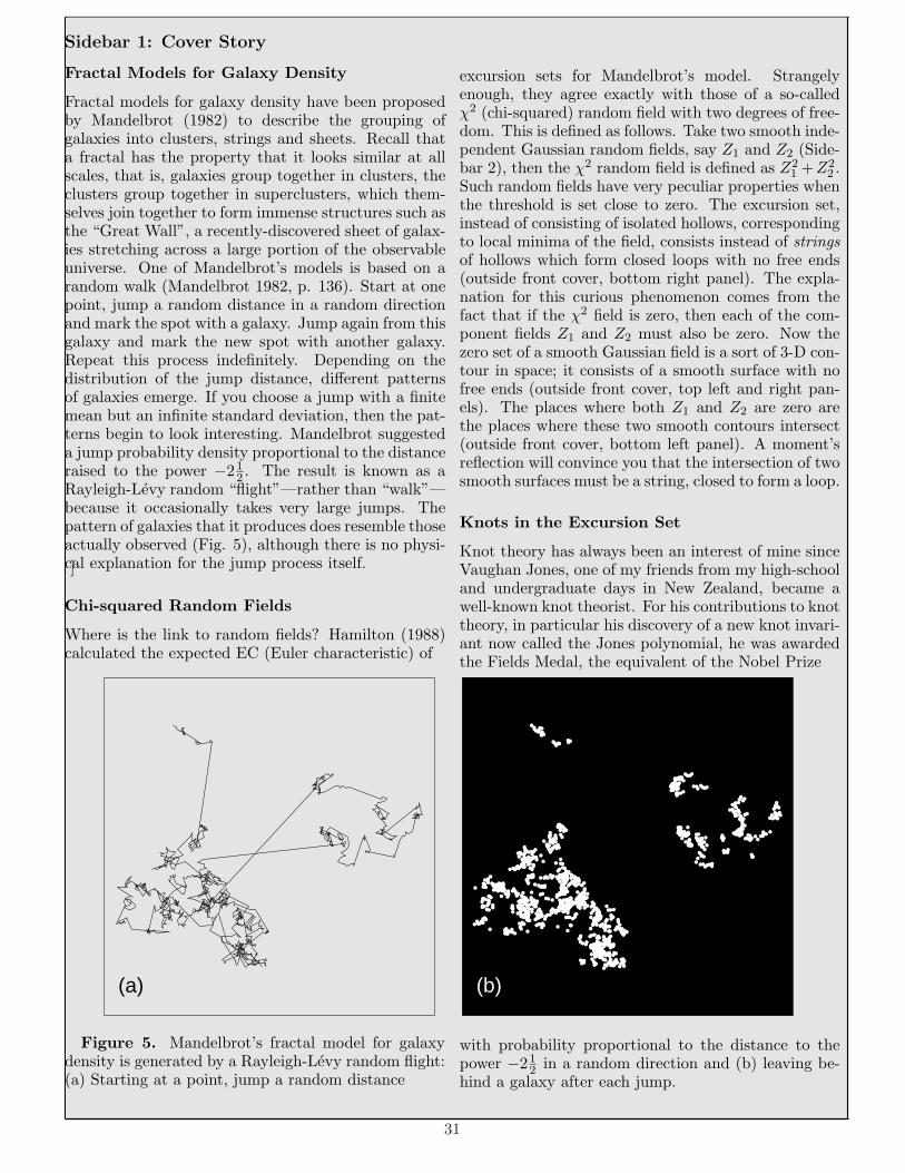
Fractal models for galaxy density have been proposedby Mandelbrot (1982) to describe the grouping ofgalaxies into clusters, strings and sheets. Recall thata fractal has the property that it looks similar at allscales, that is, galaxies group together in clusters, theclusters group together in superclusters, which them-selves join together to form immense structures such asthe “Great Wall”, a recently-discovered sheet of galax-ies stretching across a large portion of the observableuniverse. One of Mandelbrot’s models is based on arandom walk (Mandelbrot 1982, p. 136). Start at onepoint, jump a random distance in a random directionand mark the spot with a galaxy. Jump again from thisgalaxy and mark the new spot with another galaxy.Repeat this process indefinitely. Depending on thedistribution of the jump distance, different patternsof galaxies emerge. If you choose a jump with a finitemean but an infinite standard deviation, then the pat-terns begin to look interesting. Mandelbrot suggesteda jump probability density proportional to the distanceraised to the power −21

2 . The result is known as aRayleigh-Levy random “flight”—rather than “walk”—because it occasionally takes very large jumps. Thepattern of galaxies that it produces does resemble thoseactually observed (Fig. 5), although there is no physi-cal explanation for the jump process itself.

Chi-squared Random Fields

Where is the link to random fields? Hamilton (1988)calculated the expected EC (Euler characteristic) of

(a)

•••••••••••••••••••• •••

•••••••••••••••••••••••••••••

••••••••••••••

•••••••••••• ••••••••••••••••••

••••• •••••••••••••• •••• •

•••••••••••••••• •••••••• ••••••••••••••••••••••••••••••••••••••

•••••••••••••

••••••

••••••••••••••••••••••••••••

••••••••••••

•••••••••• •••••••••••••••••••

•••••••••••••

••••••••••••••

•••••••••••••••••• ••••••

•••••••

•••••• ••••••

•••••••••••••••••••

••••••••••••••••••••••••••••

•••••••• ••••••••••••••••••• ••••••••• •••••••••••••••••••

••••••••••••••••• •••••••••••

••••••••••••

••••••••••••••••

•••••••••••

•••••••••••••••••••••••••• •••••••••••••••••

•••••••••••••••••••••••••••••••••••••••••••••••••••••

••••••••••••••••• ••••• •••

••••••••••••••••••

••••••••••••• ••••••• ••••••••

••••••••••••••••••

••••••••

•••••••••••••••••••••••••••••••••

••••••••••••••••••••••••••••• •••••••• •••••••••••••• ••

••••••••••••••

•••••••••••••••••••••••• •••

••••••• ••••••

•••••

•••••••••

••••••••

••••••••••••••••••••

•••••••••••• ••••••••••••••••••••••••••••••••

• •••••••••••••• •••••••••••••••••••

••••••••••••••• •••••••••••• ••••••••••••

(b)

Figure 5. Mandelbrot’s fractal model for galaxydensity is generated by a Rayleigh-Levy random flight:(a) Starting at a point, jump a random distance

excursion sets for Mandelbrot’s model. Strangelyenough, they agree exactly with those of a so-calledχ2 (chi-squared) random field with two degrees of free-dom. This is defined as follows. Take two smooth inde-pendent Gaussian random fields, say Z1 and Z2 (Side-bar 2), then the χ2 random field is defined as Z2

1 +Z22 .

Such random fields have very peculiar properties whenthe threshold is set close to zero. The excursion set,instead of consisting of isolated hollows, correspondingto local minima of the field, consists instead of stringsof hollows which form closed loops with no free ends(outside front cover, bottom right panel). The expla-nation for this curious phenomenon comes from thefact that if the χ2 field is zero, then each of the com-ponent fields Z1 and Z2 must also be zero. Now thezero set of a smooth Gaussian field is a sort of 3-D con-tour in space; it consists of a smooth surface with nofree ends (outside front cover, top left and right pan-els). The places where both Z1 and Z2 are zero arethe places where these two smooth contours intersect(outside front cover, bottom left panel). A moment’sreflection will convince you that the intersection of twosmooth surfaces must be a string, closed to form a loop.

Knots in the Excursion Set

Knot theory has always been an interest of mine sinceVaughan Jones, one of my friends from my high-schooland undergraduate days in New Zealand, became awell-known knot theorist. For his contributions to knottheory, in particular his discovery of a new knot invari-ant now called the Jones polynomial, he was awardedthe Fields Medal, the equivalent of the Nobel Prize

with probability proportional to the distance to thepower −21

2 in a random direction and (b) leaving be-hind a galaxy after each jump.

31

]

(there is no Nobel Prize for mathematics), and he wasmade a Fellow of the Royal Society. So as soon as Ihear the word “string” I immediately think of knots.Can these zero-sets of χ2 fields ever be knotted? Thatis, is it possible for two smooth surfaces to intersectand form a knot? For a long time I thought the an-swer was no. I just couldn’t see how it could be done. Imentioned this to Vaughan one day after we had beenwind-surfing on San Francisco Bay. After he came outof the shower, he said that not only could he find such apair of surfaces, but any knot could be formed as the in-tersection of two suitably chosen smooth surfaces. Fig.3 shows how to do it for the simplest knot, the trefoil(Fig. 3a). An elementary theorem in knot theory saysthat any knot can be represented as the boundary ofa two-sided surface, its “Seifert representation” (Fig.

]

Sidebar 2. The Gaussian Random Field

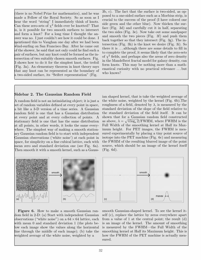
A random field is not an intimidating object; it is just aset of random variables defined at every point in space,a bit like a 3-D version of a time series. A Gaussianrandom field is one that has a Gaussian distributionat every point and at every collection of points. Astationary field is one that has the same distributionat all points, in other words, it looks the same every-where. The simplest way of making a smooth station-ary Gaussian random field is to start with independentGaussian observations (‘white noise’) at each point inspace, for simplicity on a fine cubical lattice, each withmean zero and standard deviation one (see Fig. 6a).Then smooth it with a smooth kernel, such as a Gauss-

(c)

(a)

(d)FWHM

(b)

smooth

smooth

Figure 6. How to make a smooth Gaussian ran-dom field in 2-D: (a) Start with independent Gaussianobservations (“white noise”) on a 64× 64 lattice, eachwith mean 0 and standard deviation 1 (the plots be-low each image show the values along the horizontalline through the middle of each image); (b) take theweighted average of the white noise, weighted by a

3b, c). The fact that the surface is two-sided, as op-posed to a one-sided surface such as a Moebius strip, iscrucial to the success of the proof (I have colored oneside green and the other blue). Now thicken the sur-face (Fig. 3d) and carefully cut it in half, separatingthe two sides (Fig. 3e). Now take out some sandpaperand smooth the two pieces (Fig. 3f) and push themback together so that they intersect (Fig. 3g). The in-tersection (Fig. 3h) is the knot we desire (Fig. 3i). Sothere it is . . . although there are some details to fill into complete the proof, it seems likely that the zero-setsof χ2 fields, and perhaps also the areas of zero densityin the Mandelbrot fractal model for galaxy density, canform knots. This may be nothing more than a math-ematical curiosity with no practical relevance . . . butwho knows?

ian shaped kernel, that is take the weighted average ofthe white noise, weighted by the kernel (Fig. 6b).Theroughness of a field, denoted by λ, is measured by thestandard deviation of the slope of the field relative tothe standard deviation of the field itself. It can beshown that for a Gaussian random field constructedas above, λ =

√4 loge 2/FWHM, where FWHM is the

Full Width of the smoothing kernel at Half its Max-imum height. For PET images, the FWHM is mea-sured experimentally by placing a tiny point source ofisotope into the PET machine (Fig. 6c) and measuringthe FWHM of the resulting blurred image of the pointsource, which should be an image of the kernel itself(Fig. 6d).

(c)

(a)

(d)FWHM

(b)

smooth

smooth

smooth Gaussian-shaped kernel. To see the kernel it-self (c), replace the lattice by zeros everywhere apartfrom a value of 1 at the central point; the result (d)is an image of the kernel. The amount of smoothingis measured by the FWHM—the Full Width of thesmoothing kernel at Half its Maximum height. This ishow the FWHM of the PET machine is actually mea-sured.

32

shows is that the hollows, sheets, strings, and clus-ters of galaxies might have been generated by a Gaus-sian random field model for galaxy density and thatthe meatball, sponge, and bubble topologies arise nat-urally from the model when the threshold is high,medium, or low, respectively.

Medical Images: Positron Emission Tomog-raphy

For a long time I had been doing some statistical con-sulting work for the Montreal Neurological Institute.Nothing too demanding—the odd t test or perhaps ananalysis of variance now and again. But then in thesummer of 1990 a new type of experiment was per-formed by the brain imaging center.

In this experiment, a subject is injected with a ra-dio isotope emitting positrons, which annihilate withnearby electrons to release gamma rays that are de-tected by the center’s new Positron Emission Tomog-raphy (PET) machine. By careful reconstruction, theresearchers are able to build up an image of blood flowin the brain, a measure of brain activity.

This opened up the possibility of actually seeingwhich regions of the brain were activated by differ-ent stimuli, to actually see the brain “thinking”. Fora good introduction, see the cover story of Time mag-azine, July 17, 1995.

In one of the first experiments, conducted by DanBub, a subject was told to perform a linguistic task,silent reading of words on a screen, during the imagingprocess. By subtracting an image in which the subjectwas “at rest” looking at a blank screen, the experi-menters were able to see evidence of increased bloodflow in certain brain regions corresponding to the effortrequired for the task.

The images are very blurred, however, and the signal(if any) is very weak compared to the background

Table 1: Blood-Flow at a Single Voxel

Subject Task Rest Diff.1 123.72 125.18 1.462 129.64 140.85 11.213 133.20 137.41 4.214 141.03 148.13 7.105 128.41 139.82 11.416 167.19 169.65 2.467 124.58 135.77 11.198 104.55 105.23 0.689 114.24 121.65 7.41

10 111.75 113.93 2.18mean 127.83 133.76 5.93

Voxel average s.d. = 3.61Z =

√10 mean/s.d. = 5.19

noise, so to increase the signal-to-noise ratio the exper-iment was repeated on 10 subjects. The brain imageswere aligned in 3-D, and the blood flow was averaged(see Fig. 9a, b, c).

The images are stored as values at 128 × 128 × 80locations called voxels. If we just look at one voxel, wehave 10 pairs of blood-flow values, one pair for eachsubject, one taken while the subject was performingthe task, the other while the subject was at rest. Table1 shows some values from just one voxel in the leftfrontal region of the brain.

Now comes the hard part: It looks as if some voxelsshow increased activation, but is it real or is it justdue to the noise? Here is where the statistics (and thestatistician!) come in.

Enter the Statistician—II

Any student who has been through a first course instatistics should know what to do with this sort ofdata: A paired-difference T statistic can be used tomeasure the statistical significance of the activation.This is calculated by taking the mean difference (Fig.9d), dividing by the standard deviation (s.d., Fig. 9e),and multiplying by the square root of the number ofsubjects (

√10). To increase the accuracy of the stan-

dard deviation, it was replaced by the average overall voxels to obtain a Z statistic with an approximatenormal or Gaussian distribution.

Proceeding in this way, we can make an image of Zstatistics, one for each voxel (Fig. 9f). The researchersthen scan this image, looking for high values of Z, bychoosing a threshold value t and looking at all valueswhere Z exceeds the threshold.

Now comes the tricky part: How do we choose thethreshold so that we exclude all the noise or at leastexclude it with a probability of say .95? In other words,how do we control the specificity? The first thing thatsprings to mind is to use the standard .05 critical valuesfor Z from the Normal distribution tables, which ist = 1.64 in this case. If there is really no activationat one particular voxel then the chance of finding any,that is the chance that Z > 1.64, is controlled to be.05.

But wait a minute—suppose there was really no ac-tivation anywhere in the brain, just random noise—then we would expect 5% of the voxels to exceed thisthreshold by chance alone. So if we use t = 1.64, wemight end up finding activation in at least 5% of thebrain, even when there is none at all—obviously unac-ceptable! Is there a way of correcting for this?

Students in a good course in statistics are told towatch out for “data dredging,” carrying out a multi-tude of tests and only reporting the significant ones,using the usual 5% level for each test. There are about300,000 voxels inside the brain, so we are carrying out

33

Sidebar 3: The Expected Value of the EulerCharacteristic

Our formula for the expected value of the Euler char-acteristic (EC) is remarkable because it deals with asuch a difficult random variable. How are we to applythe concept of expectation to such a curious quantityas the EC? As it turns out, there are two ways of at-tacking the problem, coming at it from two differentbranches of mathematics: differential topology and in-tegral geometry.

Differential Topology: The MathematicalMountaineer

Statisticians are used to dealing with the expectationof simple quantities such as sums of random variables.The trick is to convert the EC into just such a sum, asum of local properties of the random field, rather thanglobal properties such as connectedness. The necessarytheoretical result needed to perform this comes fromdifferential topology and Morse theory, discovered inthe 1960s. It is easiest to state in 2-D, where it sayssimply this: provided the excursion set does not touchthe boundary of the search region, then the EC of theexcursion set equals the number of local maxima of the

(a) (b)

M

M

M

M

S

S

S

S

m

(c)

M

M

M

M

S

S

(d)

M

M

M

M

(e)

M

••••••••

••••

••••••••••••••••••

•••••••••••

••••••

•••••••••••••••••••••••••••••••••••••••••••

•••

•••••••••••

•••••••••••••••••

••••••••••••••

••••••••••••••••••

••••••••

(f)threshold, t

EC

0 1 2 3 4 5 6

-2-1

01

23

4

(b)

(c)

(d)

(e)

colour bar

Figure 7. The EC of the excursion set of a randomfield in 2-D is the number of maxima (M) – saddles(S) + minima (m) of the field inside the excursion set.For an artificial image (a), the EC of the excursion setfor a low threshold (b) at t = 1 is EC = 4− 4 + 1 = 1;(c) at t = 2.8 the local minimum disappears, leaving ahole, and EC = 4− 2 + 0 = 2; (d) at t = 3.2 the hole

random field inside the excursion set, plus the numberof local minima, minus the number of saddle points (Fig. 7):

EC = #maxima−#saddles + #minima.

The mathematical mountaineer applies this result asfollows: count the number of peaks, minus the numberof saddles, plus the number of basins above a certainaltitude; the result is always the number of connectedmountain ranges above this altitude, minus the num-ber of lower altitude plains completely surrounded bymountains. In other words, the mountain heights formthe random field, the peaks are maxima, the basins areminima, the saddles are just the saddles, and the excur-sion set is the places above a fixed altitude. Now placea +1 at every local maximum and local minimum, a−1 at every saddle point, and a 0 at every other point;add these up and you have the EC. The expected ECis then just the sum of the expected +1,−1, or 0 atevery point, which leads, after a lot of delicate manip-ulation, to the first term of the expected EC, the partdiscovered by Robert Adler. There is only one snag:what happens if the excursion set touches the bound-ary? For this possibility, a special boundary correctionis required that adds three more terms to Adler’s re-

breaks open leaving components with just one localmaximum in each, and EC = 4− 0 + 0 = 4; (e) at t =5.6, just below the global maximum, EC = 1−0+0 = 1;above the global maximum the EC is 0, so that for highthresholds the expected EC approximates the p valueof the global maximum; (f) is a plot of the EC againstthe threshold, t.

34

sult. These can also be obtained by counting localmaxima and minima on the boundary, and follow-ing the same delicate manipulation in Adler’s originalproof. An alternative method of proof, using integralgeometry, is given in the next section.

Integral Geometry: Buffon’s Needle

One branch of integral geometry, called stereology,concerns the number of times that a randomly placedobject intersects a fixed object. Scientists use theseresults to infer the shape of 3-D objects such as cellsthat are viewed only as 2-D slices in a microscope. Itall began with Georges Louis Leclerc Comte de Buffon(1707–1788), a French naturalist, who wrote L’HistoireNaturelle, one of the most widely-read scientific worksof the 18th century. He is best known to mathemati-cians for his method of calculating π by simply throw-ing a needle at random onto the floor and counting theproportion of times r, say, that it crossed the cracksbetween the floor boards (Fig. 8a). If the needle hasthe same length as the width of the floor boards, thenhe showed that the probability of crossing the cracksequals 2/π, so that π is approximated by 2/r. A gen-

(a) (b)

Figure 8. A generalization of Buffon’s needle isused to find the formula for the expected EC of theexcursion set; (a) a needle is thrown at random ontothe floor; if the length of the needle is the same as theseparation of the cracks in the floor boards, then theprobability of the needle crossing a crack is 2/π; (b)

eralization of this result was discovered by Blaschkein the mid-1930s, where the needle and the cracks arereplaced by two arbitrary sets A and B in 3-D, andthe proportion of crosses is replaced by the total ECof the set of points that belong to both sets. The re-sult, known as the Kinematic Fundamental Formula—“Fundamental” because it underlies so many other re-sults in integral geometry—is as follows:

∫EC = 8π2(Volume ofA)(EC ofB)

+ 4π2(Area ofA)(Diameter ofB)+ 4π2(Diameter ofA)(Area ofB)+ 8π2(EC ofA)(Volume ofB).

Now we extend the random field out on all sides be-yond the search region, hold it fixed, and use the ex-cursion set as the “cracks” (B). Onto this we drop arandom search region (A) that becomes the “needle”(Fig. 8b). The Kinematic Fundamental Formula thengives an expression for the expected EC, which aftera little more manipulation becomes the four terms ofthe result we want.

replace the needle with the search region (shown in 2-D) and the cracks with the excursion set of a randomfield, extended on all sides; the Kinematic Fundamen-tal Formula gives the expected EC of the points incommon (black), which leads eventually to the formulawe want.

35

(a) (b) (c)

(d) (e) (f)

(g) (h)

Figure 10. The anomalies in the cosmic microwavebackground radiation—thought to be the signature ofthe creation of the universe by the “big bang.” The

anomalies were discovered in 1992 by George Smootand his coworkers at the Lawrence Berkeley Laborato-ries.

36

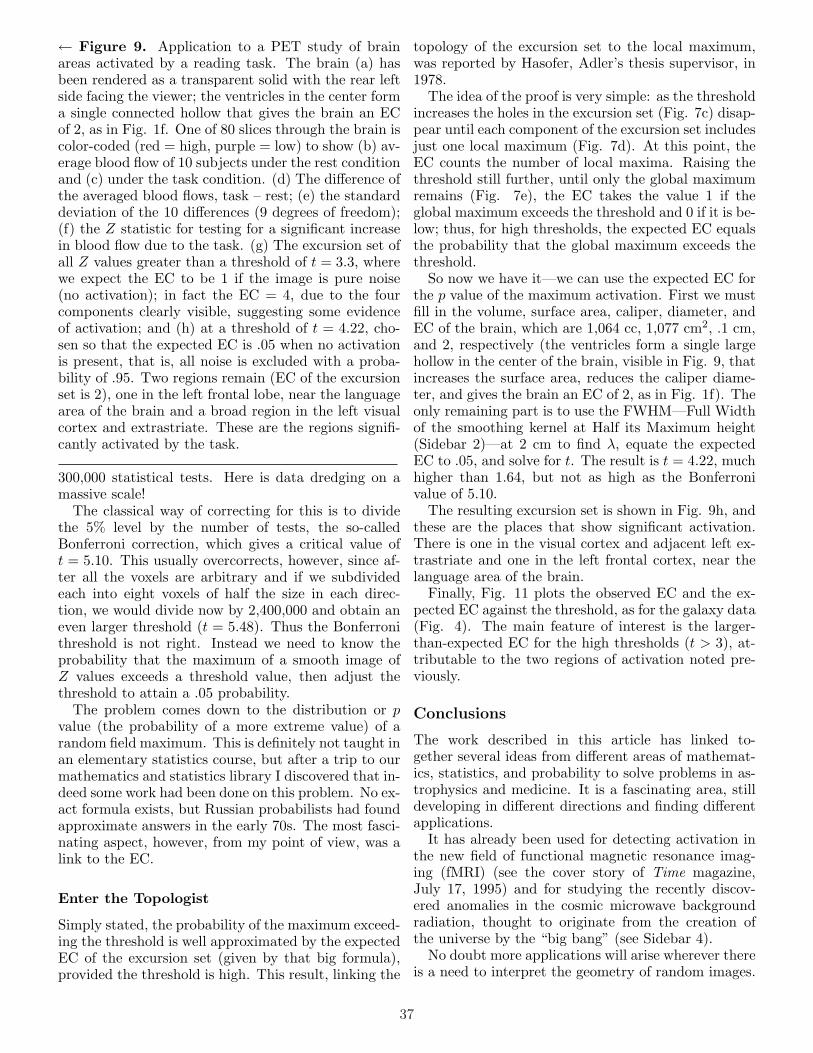
← Figure 9. Application to a PET study of brainareas activated by a reading task. The brain (a) hasbeen rendered as a transparent solid with the rear leftside facing the viewer; the ventricles in the center forma single connected hollow that gives the brain an ECof 2, as in Fig. 1f. One of 80 slices through the brain iscolor-coded (red = high, purple = low) to show (b) av-erage blood flow of 10 subjects under the rest conditionand (c) under the task condition. (d) The difference ofthe averaged blood flows, task – rest; (e) the standarddeviation of the 10 differences (9 degrees of freedom);(f) the Z statistic for testing for a significant increasein blood flow due to the task. (g) The excursion set ofall Z values greater than a threshold of t = 3.3, wherewe expect the EC to be 1 if the image is pure noise(no activation); in fact the EC = 4, due to the fourcomponents clearly visible, suggesting some evidenceof activation; and (h) at a threshold of t = 4.22, cho-sen so that the expected EC is .05 when no activationis present, that is, all noise is excluded with a proba-bility of .95. Two regions remain (EC of the excursionset is 2), one in the left frontal lobe, near the languagearea of the brain and a broad region in the left visualcortex and extrastriate. These are the regions signifi-cantly activated by the task.

300,000 statistical tests. Here is data dredging on amassive scale!

The classical way of correcting for this is to dividethe 5% level by the number of tests, the so-calledBonferroni correction, which gives a critical value oft = 5.10. This usually overcorrects, however, since af-ter all the voxels are arbitrary and if we subdividedeach into eight voxels of half the size in each direc-tion, we would divide now by 2,400,000 and obtain aneven larger threshold (t = 5.48). Thus the Bonferronithreshold is not right. Instead we need to know theprobability that the maximum of a smooth image ofZ values exceeds a threshold value, then adjust thethreshold to attain a .05 probability.

The problem comes down to the distribution or pvalue (the probability of a more extreme value) of arandom field maximum. This is definitely not taught inan elementary statistics course, but after a trip to ourmathematics and statistics library I discovered that in-deed some work had been done on this problem. No ex-act formula exists, but Russian probabilists had foundapproximate answers in the early 70s. The most fasci-nating aspect, however, from my point of view, was alink to the EC.

Enter the Topologist

Simply stated, the probability of the maximum exceed-ing the threshold is well approximated by the expectedEC of the excursion set (given by that big formula),provided the threshold is high. This result, linking the

topology of the excursion set to the local maximum,was reported by Hasofer, Adler’s thesis supervisor, in1978.

The idea of the proof is very simple: as the thresholdincreases the holes in the excursion set (Fig. 7c) disap-pear until each component of the excursion set includesjust one local maximum (Fig. 7d). At this point, theEC counts the number of local maxima. Raising thethreshold still further, until only the global maximumremains (Fig. 7e), the EC takes the value 1 if theglobal maximum exceeds the threshold and 0 if it is be-low; thus, for high thresholds, the expected EC equalsthe probability that the global maximum exceeds thethreshold.

So now we have it—we can use the expected EC forthe p value of the maximum activation. First we mustfill in the volume, surface area, caliper, diameter, andEC of the brain, which are 1,064 cc, 1,077 cm2, .1 cm,and 2, respectively (the ventricles form a single largehollow in the center of the brain, visible in Fig. 9, thatincreases the surface area, reduces the caliper diame-ter, and gives the brain an EC of 2, as in Fig. 1f). Theonly remaining part is to use the FWHM—Full Widthof the smoothing kernel at Half its Maximum height(Sidebar 2)—at 2 cm to find λ, equate the expectedEC to .05, and solve for t. The result is t = 4.22, muchhigher than 1.64, but not as high as the Bonferronivalue of 5.10.

The resulting excursion set is shown in Fig. 9h, andthese are the places that show significant activation.There is one in the visual cortex and adjacent left ex-trastriate and one in the left frontal cortex, near thelanguage area of the brain.

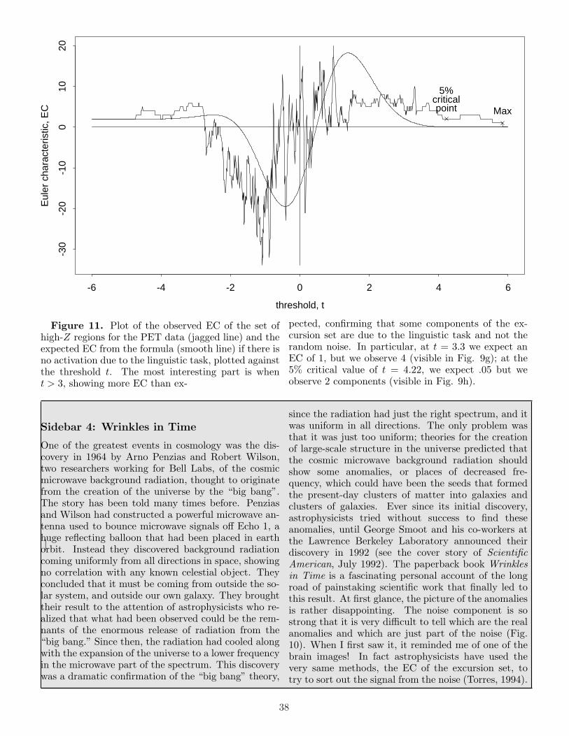
Finally, Fig. 11 plots the observed EC and the ex-pected EC against the threshold, as for the galaxy data(Fig. 4). The main feature of interest is the larger-than-expected EC for the high thresholds (t > 3), at-tributable to the two regions of activation noted pre-viously.

Conclusions

The work described in this article has linked to-gether several ideas from different areas of mathemat-ics, statistics, and probability to solve problems in as-trophysics and medicine. It is a fascinating area, stilldeveloping in different directions and finding differentapplications.

It has already been used for detecting activation inthe new field of functional magnetic resonance imag-ing (fMRI) (see the cover story of Time magazine,July 17, 1995) and for studying the recently discov-ered anomalies in the cosmic microwave backgroundradiation, thought to originate from the creation ofthe universe by the “big bang” (see Sidebar 4).

No doubt more applications will arise wherever thereis a need to interpret the geometry of random images.

37

threshold, t

Eul

er c

hara

cter

istic

, EC

-6 -4 -2 0 2 4 6

-30

-20

-10

010

20

5%criticalpoint Max

Figure 11. Plot of the observed EC of the set ofhigh-Z regions for the PET data (jagged line) and theexpected EC from the formula (smooth line) if there isno activation due to the linguistic task, plotted againstthe threshold t. The most interesting part is whent > 3, showing more EC than ex-

]

Sidebar 4: Wrinkles in Time

One of the greatest events in cosmology was the dis-covery in 1964 by Arno Penzias and Robert Wilson,two researchers working for Bell Labs, of the cosmicmicrowave background radiation, thought to originatefrom the creation of the universe by the “big bang”.The story has been told many times before. Penziasand Wilson had constructed a powerful microwave an-tenna used to bounce microwave signals off Echo 1, ahuge reflecting balloon that had been placed in earthorbit. Instead they discovered background radiationcoming uniformly from all directions in space, showingno correlation with any known celestial object. Theyconcluded that it must be coming from outside the so-lar system, and outside our own galaxy. They broughttheir result to the attention of astrophysicists who re-alized that what had been observed could be the rem-nants of the enormous release of radiation from the“big bang.” Since then, the radiation had cooled alongwith the expansion of the universe to a lower frequencyin the microwave part of the spectrum. This discoverywas a dramatic confirmation of the “big bang” theory,

pected, confirming that some components of the ex-cursion set are due to the linguistic task and not therandom noise. In particular, at t = 3.3 we expect anEC of 1, but we observe 4 (visible in Fig. 9g); at the5% critical value of t = 4.22, we expect .05 but weobserve 2 components (visible in Fig. 9h).

since the radiation had just the right spectrum, and itwas uniform in all directions. The only problem wasthat it was just too uniform; theories for the creationof large-scale structure in the universe predicted thatthe cosmic microwave background radiation shouldshow some anomalies, or places of decreased fre-quency, which could have been the seeds that formedthe present-day clusters of matter into galaxies andclusters of galaxies. Ever since its initial discovery,astrophysicists tried without success to find theseanomalies, until George Smoot and his co-workers atthe Lawrence Berkeley Laboratory announced theirdiscovery in 1992 (see the cover story of ScientificAmerican, July 1992). The paperback book Wrinklesin Time is a fascinating personal account of the longroad of painstaking scientific work that finally led tothis result. At first glance, the picture of the anomaliesis rather disappointing. The noise component is sostrong that it is very difficult to tell which are the realanomalies and which are just part of the noise (Fig.10). When I first saw it, it reminded me of one of thebrain images! In fact astrophysicists have used thevery same methods, the EC of the excursion set, totry to sort out the signal from the noise (Torres, 1994).

38

]

In this case, the search region is the surface of a unitsphere, so the volume is zero, the surface area is 8π2

(4π2 for the inside and 4π2 for the outside), the caliperdiameter is zero, and the EC of the search region is 2(because it is a hollow sphere, like a tennis ball). Wecan use these results to calculate the expected EC andto plot it and the observed EC against threshold level

threshold, t

Eul

er c

hara

cter

istic

, EC

-4 -3 -2 -1 0 1 2 3 4

-80

-60

-40

-20

020

4060

80

Figure 12. Plot of the observed EC of excursionsets of the anomalies in the cosmic microwave back-ground radiation (jagged line), and the expected ECfrom the formula (smooth line) if there are no realanomalies. The observed microwave background radi-ation produces an EC curve similar in shape to that

References and Further Reading

Adler, R. J. (1981), The Geometry of Random Fields, NewYork: John Wiley.

Buffon, G. L. L., Comte de (1777), “Essai d’ArithmetiqueMorale,” Supplement a l’Histoire Naturelle, Tome 4.

Hamilton, A. J. S. (1988) “The Topology of Fractal Uni-verses,” Publications of the Astronomical Society of thePacific, 100, 1343–1350.

Mandelbrot, B. B. (1982), The Fractal Geometry of Na-ture, New York: W. H. Freeman.

Smoot, G., and Davidson, K. (1993), Wrinkles in Time,New York: William Morrow.

Torres, S. (1994), “Topological Analysis of COBE-DMRCosmic Microwave Background Maps,” Astrophysical

(Fig. 12). The observed microwave background radia-tion produces an EC curve similar in shape to thatexpected, but somewhat lower and spread more inthe tails. This discrepancy points to a Gaussian ran-dom field model for the anomalies, with a larger stan-dard deviation and a larger smoothness than the back-ground noise.

expected, but somewhat lower and spread more in thetails—evidence that some of the anomalies are real andnot just due to random noise. This discrepancy pointsto a Gaussian random field model for the anomalies,with a larger standard deviation and a larger smooth-ness than the background noise.

Journal, 423, L9–L12.

Vogeley, M. S., Park, C., Geller, M. J., Huchira, J. P., andGott, J. R. (1994), “Topological Analysis of the CfARedshift Survey,” Astrophysical Journal, 420, 525–544.

Worsley, K. J. (1995), “Estimating the Number of Peaks ina Random Field Using the Hadwiger Characteristic ofExcursion Sets, with Applications to Medical Images,”The Annals of Statistics, 23, 640–669.

Worsley, K. J. (1995), “Boundary Corrections for the Ex-pected Euler Characteristic of Excursion Sets of Ran-dom Fields, With an Application to Astrophysics,” Ad-vances in Applied Probability, 27, 943–959.

Worsley, K. J., Evans, A. C., Marrett, S., and Neelin, P.(1992), “A Three Dimensional Statistical Analysis forCBF Activation Studies in Human Brain,” Journal ofCerebral Blood Flow and Metabolism, 12, 900–918.

39