arX

iv:a

stro

-ph/

0309

411v

2 1

Dec

200

3

Chameleon Cosmology

Justin Khoury and Amanda Weltman

Institute for Strings, Cosmology and Astroparticle Physics, Columbia University, New York, NY 10027

The evidence for the accelerated expansion of the universe and the time-dependence of the fine-

structure constant suggests the existence of at least one scalar field with a mass of order H0. If such

a field exists, then it is generally assumed that its coupling to matter must be tuned to unnaturally

small values in order to satisfy the tests of the Equivalence Principle (EP). In this paper, we present

an alternative explanation which allows scalar fields to evolve cosmologically while having couplings

to matter of order unity. In our scenario, the mass of the fields depends on the local matter density:

the interaction range is typically of order 1 mm on Earth (where the density is high) and of order

10−104 AU in the solar system (where the density is low). All current bounds from tests of General

Relativity are satisfied. Nevertheless, we predict that near-future experiments that will test gravity

in space will measure an effective Newton’s constant different by order unity from that on Earth,

as well as EP violations stronger than currently allowed by laboratory experiments. Such outcomes

would constitute a smoking gun for our scenario.

I. INTRODUCTION

There is growing evidence in cosmology for the existence of nearly massless scalar fields in our Universe. On

the one hand, a host of observations, from supernovae luminosity-distance measurements [1] to the cosmic microwave

background anisotropy [2], suggests that 70% of the current energy budget consists of a dark energy fluid with negative

pressure. While observations are consistent with a non-zero cosmological constant, the dark energy component is more

generally modeled as quintessence: a scalar field rolling down a flat potential [3, 4]. In order for the quintessence field

to be evolving on cosmological time scales today, its mass must be of order H0, the present Hubble parameter.

On the other hand, recent measurements of absorption lines in quasar spectra suggest that the fine-structure

constant α has evolved by roughly one part in 105 over the redshift interval 0.2 < z < 3.7 [5]. Time-variation of

coupling constants are generally modeled with rolling scalar fields [6], and the recent evidence for a time-varying α

requires the mass of the corresponding scalar field to be of order H0 [7].

In either case, the inferred scalar field is essentially massless on solar system scales, and therefore subject to tight

constraints from tests of the Equivalence Principle (EP) [8]. The current bound on the Eotvos parameter, η, which

quantifies the deviation from the universality of free-fall, is η < 10−13, from the Eot-Wash experiment [9].

From a theoretical standpoint, massless scalar fields or moduli are abundant in string and supergravity theories.

Indeed, generic compactifications of string theory result in a plethora of massless scalars in the low-energy, four-

dimensional effective theory. However, these massless fields generally couple directly to matter with gravitational

strength, and therefore lead to unacceptably large violations of the EP. Therefore, if the culprit for quintessence

or time-varying α is one of the moduli of string theory, some mechanism must effectively suppress its EP-violating

contributions.

For instance, Damour and Polyakov [10] (see also [11]) have proposed a dynamical mechanism to suppress the

coupling constants βi between the various matter fields and the dilaton of string theory. Alternatively, the suppression

2

could be the result of approximate global symmetries [12].

In a recent paper [13], we presented a scenario in which scalar fields can evolve cosmologically while having couplings

to matter of order unity, i.e., βi ∼ O(1). This is because the scalar fields acquire a mass whose magnitude depends

on the local matter density. In a region of high density, such as on Earth, the mass of the fields is large, and thus the

resulting violations of the EP are exponentially suppressed. In the solar system, where the density is much lower, the

moduli are essentially free, with a Compton wavelength that can be much larger than the size of the solar system.

Finally, on cosmological scales, where the density is very low, the mass can be of the order of the present Hubble

parameter, thereby making the fields potential candidates for causing the acceleration of the universe or the time-

evolution of the fine-structure constant. While the idea of density-dependent mass terms is not new [10, 14, 15, 16],

the novelty of our work lies in that the scalar fields can couple directly to baryons with gravitational strength.

In our scenario, scalar fields that have cosmological effects, such as quintessence, do not result in large violations of

the EP in the laboratory because we happen to live in a very dense environment. Thus, the main constraint on our

model is that the mass of the field be sufficiently large on Earth to evade EP and fifth force constraints [17].

The generation of a density-dependent mass for a given modulus φ results from the interplay of two source terms in

its equation of motion. The first term arises from self-interactions, described by a monotonically-decreasing potential

V (φ) which is of the runaway form (see Fig. 1). In particular, we underscore the fact that the potential need not

have a minimum; rather, it must be monotonic. The second term arises from the conformal coupling to matter fields,

of the form eβiφ/MP l . The coupling constants βi need not be small, however, and values of order unity or greater

are allowed. Although these two contributions are both monotonic functions of φ, their combined effect is that of

an effective potential which does display a minimum (see Fig. 2). Furthermore, since this effective potential depends

explicitly on the local matter density ρ, both the field value at the minimum and the mass of small fluctuations depend

on ρ as well, with the latter being an increasing function of the density.

Although the scalar fields are quite massive on Earth, their behavior is strikingly different in the solar system where

the local matter density is much smaller. Thus our model makes a crucial prediction for near-future experiments

that will test gravity in space. For example, consider the SEE Project [18] which among other things will measure

Newton’s constant to an unprecedented accuracy. Our scenario generically predicts that the SEE experiment should

observe corrections of order unity to Newton’s constant compared to its measured value on Earth, due to fifth-force

contributions which are important in space but exponentially suppressed on Earth.

Moreover, three satellite experiments to be launched in the near future, STEP [19], Galileo Galilei (GG) [20] and

MICROSCOPE [21], will test the universality of free-fall in orbit with expected accuracy of 10−18, 10−17 and 10−15,

respectively. We predict that these experiments should observe a strong EP-violating signal. In fact, for a wide range

of parameters, our model predicts that the signal will be larger than the ground-based Eot-Wash bound of 10−13.

If SEE does measure an effective Newton’s constant different from that on Earth, or if STEP observes an EP-

violating signal larger than thought permitted by the Eot-Wash experiment, this will strongly indicate that a mech-

anism of the form proposed here is realized in Nature. For otherwise it would be hard to explain the discrepancies

between measurements in the laboratory and those in orbit. These new and surprising outcomes are a direct conse-

quence of the fact that scalar fields in our model have drastically different behavior in regions of high density than in

regions of low density.

We refer to φ as a “chameleon” field, since its physical properties, such as its mass, depend sensitively on the envi-

3

ronment. Moreover, in regions of high density, the chameleon “blends” with its environment and becomes essentially

invisible to searches for EP violation and fifth force.

Even though we predict significant violations of the EP in space, all existing constraints from planetary orbits [8],

such as those from lunar laser ranging [22], are easily satisfied in our model. This is because of the fact that the

chameleon-mediated force between two large objects, such as the Earth and the Sun, is much weaker than one would

naively expect. To see this, we use calculus and break up the Earth into a collection of infinitesimal volume elements.

Consider one such volume element located well-within the Earth. Since the mass of the chameleon is very large inside

the Earth, the φ-flux from this volume element is exponentially suppressed and therefore contributes negligibly to the

φ-field outside the Earth. This is true for all volume elements within the Earth, except for those located in a thin shell

near the surface. Infinitesimal elements within this shell are so close to the surface that they do not suffer from the

bulk exponential suppression. Thus, the exterior field is generated almost entirely by this thin shell, whereas the bulk

of the Earth contributes negligibly. A similar argument applies to the Sun. Consequently, the chameleon-mediated

force between the Earth and the Sun is suppressed by this thin-shell effect, which thereby ensures that solar system

tests of gravity are satisfied.

However, note that this only applies to large objects, such as planets. Sufficiently small objects do not suffer from

thin-shell suppression, and thus their entire mass contributes to the exterior field. In particular, a small satellite in

orbit, such as SEE, may not exhibit a thin-shell effect. This is why the orbits of the planets are essentially unaffected

by the φ-force, whereas the fifth force between two test particles in the SEE capsule is significant.

Since φ couples directly to matter fields, all mass scales and coupling constants of the Standard Model depend on

space and time. Once again due to the thin-shell mechanism described above, spatial variations of constants are suffi-

ciently small in our model to satisfy current experimental bounds, for instance from the Vessot-Levine experiment [23].

Time variation of coupling constants are also not a problem since, during most of the history of the universe, the

various couplings actually change by very little. Thus the bounds from big bang nucleosynthesis, for instance, are

easily satisfied. This will be described in more detail in a separate paper dealing with the cosmological evolution in

our model [24].

In Sec. II, we describe the ingredients of the scenario, focusing on a single modulus φ for simplicity. We show how

the dynamics of φ are governed by an effective potential that depends on the local matter density. In Sec. III, we

derive approximate solutions for φ for a compact object such as the Sun, for instance, and describe the thin-shell

mechanism mentioned earlier. In Sec. IV, we specialize the solution for φ to the case of the Earth, and apply the

results in Sec. V to derive constraints on the parameters of the theory based on laboratory tests of the EP and searches

for a fifth force. We then show in Sec. VI that, for a potential of power-law form, V (φ) = M4+nφ−n, these constraints

translate into the requirement that the energy scale M be less than an inverse millimeter or so. Curiously, this is

also the scale associated with the cosmological constant today. In Sec. VII, we argue that our model easily satisfies

constraints from solar system tests of GR. It is showed (Sec. VIII) that the same holds true for bounds from spatial

and time variation of coupling constants. We then predict (Sec. IX) that near-future experiments that aim at testing

the EP and measuring a fifth force should observe a large signal, perhaps stronger than previously thought possible.

Finally, we conclude and summarize our results in Sec. X.

4

V(φ)

φFIG. 1: Example of a runaway potential.

II. THE INGREDIENTS OF THE MODEL

Focusing on a single scalar field φ for simplicity, the action governing the dynamics of our model is given by

S =

∫

d4x√−g

{

M2Pl

2R− 1

2(∂φ)2 − V (φ)

}

−∫

d4xLm(ψ(i)m , g(i)

µν) , (1)

where MPl ≡ (8πG)−1/2 is the reduced Planck mass, g is the determinant of the metric gµν , R is the Ricci scalar and

ψ(i)m are matter fields. The scalar field φ interacts directly with matter particles through a conformal coupling of the

form eβiφ/MP l . Explicitly, each matter field ψ(i)m couples to a metric g

(i)µν which is related to the Einstein-frame metric

gµν by the rescaling

g(i)µν = e2βiφ/MP lgµν , (2)

where βi are dimensionless constants [25]. Moreover, for simplicity, we assume that the different ψ(i)m ’s do not interact

with each other. Note that Eq. (1) is of the general form of low-energy effective actions from string theory and

supergravity, where V (φ) arises from non-perturbative effects.

The potential V (φ) is assumed to be of the runaway form. That is, it is monotonically decreasing and satisfies

limφ→∞

V = 0 , limφ→∞

V,φ

V= 0 , lim

φ→∞

V,φφ

V,φ= 0 . . . , (3)

as well as

limφ→0

V = ∞ , limφ→0

V,φ

V= ∞ , lim

φ→0

V,φφ

V,φ= ∞ . . . , (4)

where V,φ ≡ dV/dφ, etc. See Fig. 1. For instance, a fiducial example is the inverse power-law potential

V (φ) = M4+nφ−n , (5)

where M has units of mass and n is a positive constant. The above conditions on the asymptotics of V are generally

satisfied by potentials arising from non-perturbative effects in string theory [14, 15, 16, 26]. Note that it is also of the

desired form for quintessence models of the universe [27].

5

The equation of motion for φ derived from the above action is then

∇2φ = V,φ −∑

i

βi

MPle4βiφ/MP lgµν

(i)T(i)µν , (6)

where T(i)µν = (2/

√

−g(i))δLm/δgµν(i) is the stress-energy tensor for the ith form of matter. For the purpose of this

paper, it will suffice to approximate the geometry as Minkowski space, that is, gµν ≈ ηµν . This is valid provided that

the Newtonian potential is small everywhere, and that the backreaction due to the energy density in φ is also small.

This latter assumption will be justified when we analyze post-Newtonian corrections in Sec. VII B.

For non-relativistic matter, one has gµν(i)T

(i)µν ≈ −ρi, where ρi is the energy density. However, we shall find it

convenient to express our equations not in terms of ρi, but rather in terms of an energy density ρi ≡ ρie3βiφ/MP l

which is conserved in Einstein frame. In other words, ρi is defined so that it is independent of φ. Equation (6) thus

reduces to

∇2φ = V,φ +∑

i

βi

MPlρie

βiφ/MP l . (7)

From the right-hand side of Eq. (7), we see that the dynamics of φ are not solely governed by V (φ), but rather by

an effective potential

Veff (φ) ≡ V (φ) +∑

i

ρieβiφ/MP l (8)

which depends explicitly on the matter density ρi. In particular, although V (φ) is monotonic, Veff does exhibit a

minimum provided that βi > 0. This is illustrated in Fig. 2 for the case of a single component ρ with coupling β.

(One could equivalently consider the case V,φ > 0 and βi < 0.) Unfortunately, known examples in string theory have

V,φ and βi occurring with the same sign. If φ is the modulus of an extra dimension, for instance, then one expects

that V → 0 and V,φ → 0 in the decompactification limit [28]; in this limit, the various masses of particles also tend

to zero.

We will denote by φmin the value assumed by φ at the minimum, that is,

V,φ(φmin) +∑

i

βi

MPlρie

βiφmin/MP l = 0 . (9)

Meanwhile, the mass of small fluctuations about φmin is obtained as usual by evaluating the second derivative of the

potential at φmin:

m2min = V,φφ(φmin) +

∑

i

β2i

M2Pl

ρieβiφmin/MP l . (10)

Equations (9) and (10) respectively imply that the local value of the field, φmin, and its mass, mmin, both depend

on the local matter density. Since V,φ is negative and monotonically increasing, while V,φφ is positive and decreasing,

it also follows that larger values of ρi correspond to smaller φmin and larger mmin. This is illustrated in Fig. 3.

The denser the environment, the more massive is the chameleon. We will later see that it is possible for mmin to be

sufficiently large on Earth to evade current constraints on EP violations and fifth force, while being sufficiently small

on cosmological scales for φ to have interesting cosmological effects.

The upshot of our model, from a theoretical standpoint, is that the potential V (φ) need not have a minimum, nor

does the coupling constant β need be tuned to less than 10−4 to satisfy EP constraints [10]. Quite the contrary, V (φ)

is assumed monotonic, while β can be of order unity.

6

ρ

φ)V(

effV (φ)

φ

Mβ φ/ )Plexp(

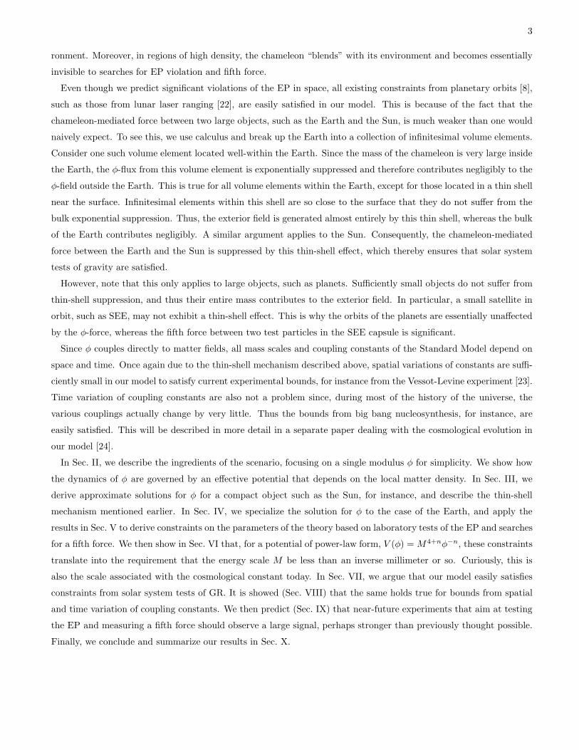
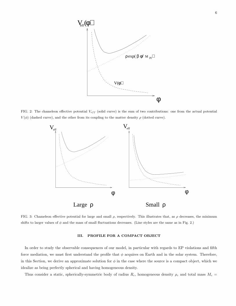
FIG. 2: The chameleon effective potential Veff (solid curve) is the sum of two contributions: one from the actual potential

V (φ) (dashed curve), and the other from its coupling to the matter density ρ (dotted curve).

φφ

Veff

ρSmallρLarge

Veff

FIG. 3: Chameleon effective potential for large and small ρ, respectively. This illustrates that, as ρ decreases, the minimum

shifts to larger values of φ and the mass of small fluctuations decreases. (Line styles are the same as in Fig. 2.)

III. PROFILE FOR A COMPACT OBJECT

In order to study the observable consequences of our model, in particular with regards to EP violations and fifth

force mediation, we must first understand the profile that φ acquires on Earth and in the solar system. Therefore,

in this Section, we derive an approximate solution for φ in the case where the source is a compact object, which we

idealize as being perfectly spherical and having homogeneous density.

Thus consider a static, spherically-symmetric body of radius Rc, homogeneous density ρc and total mass Mc =

7

4πR3cρc/3. In the case of the Earth, the latter can be approximated by the characteristic terrestrial density: ρ⊕ ≈

10 g/cm3. We treat the object as isolated, in the sense that the effect of surrounding bodies is neglected. It is

not in vacuum, however, but is instead immersed in a background of homogeneous density ρ∞. In the case of solar

system objects, this models the fact that our local neighborhood of the galaxy is not empty, but rather filled with

an approximately homogeneous component of baryonic gas and dark matter with density ρ∞ ≡ ρG ≈ 10−24 g/cm3.

In the case of a baseball in the Earth’s atmosphere, ρ∞ denotes the surrounding atmospheric density: ρ∞ ≡ ρatm ≈10−3 g/cm3.

With these assumptions, Eq. (7) reduces to

d2φ

dr2+

2

r

dφ

dr= V,φ +

β

MPlρ(r)eβφ/MP l , (11)

where

ρ(r) =

ρc for r < Rc

ρ∞ for r > Rc

. (12)

Note that we temporarily focus on the case where all βi’s assume the same value β. This is done for simplicity

only, and the following analysis remains qualitatively unchanged when these are taken to be different. Moreover, this

assumption will be dropped when we derive the resulting violations of the EP in Sec. V. In other words, in the end

we are not assuming that the theory is Brans-Dicke [29].

Throughout the analysis, we denote by φc and φ∞ the field value which minimizes Veff for r < Rc and r > Rc,

respectively. That is, from Eqs. (9) and (12), we have

V,φ(φc) +β

MPlρce

βφc/MP l = 0 ;

V,φ(φ∞) +β

MPlρ∞e

βφ∞/MP l = 0 . (13)

Similarly, we denote by mc and m∞ the mass of small fluctuations about φc and φ∞, respectively. That is, mc (m∞)

is the mass of the chameleon field inside (outside) the object.

Equation (11) is a second order differential equation and as such requires two boundary conditions. Since the

solution must be non-singular at the origin, we require dφ/dr = 0 at r = 0, as usual. Moreover, since ρ = ρ∞ at

infinity, it is natural to impose φ→ φ∞ as r → ∞. This latter condition is physically sensible as it implies dφ/dr → 0

as r → ∞, and thus that the φ-force between the compact object and a test particle tends to zero as their separation

becomes infinite. To summarize, Eq. (11) is subject to the following two boundary conditions:

dφ

dr= 0 at r = 0 ;

φ→ φ∞ as r → ∞ . (14)

A. Qualitative description of the solution

Before solving this problem explicitly, it is useful to give a heuristic derivation of the solution. Far outside the

object, r ≫ Rc, we know that the chameleon tends to φ∞, as required by the second boundary condition. There are

then two types of solution, depending on whether the object is large (e.g., the Earth) or small (e.g., a baseball). The

distinction between large and small will be made precise below.

8

r~

������������������������������������������������������������������������������������������������������������������������������������������������������������������������������������������������������������������������������������������������������������������������������������������������������������������������������������������������������������������������������������������������������������������������������������������������������������������������������������������������������������������������������������������������������������������������������������������������������������������������������������������������������������������������������������������������������������

������������������������������������������������������������������������������������������������������������������������������������������������������������������������������������������������������������������������������������������������������������������������������������������������������������������������������������������������������������������������������������������������������������������������������������������������������������������������������������������������������������������������������������������������������������������������������������������������������������������������������������������������������������������������������������������������������������

r

dV

R c

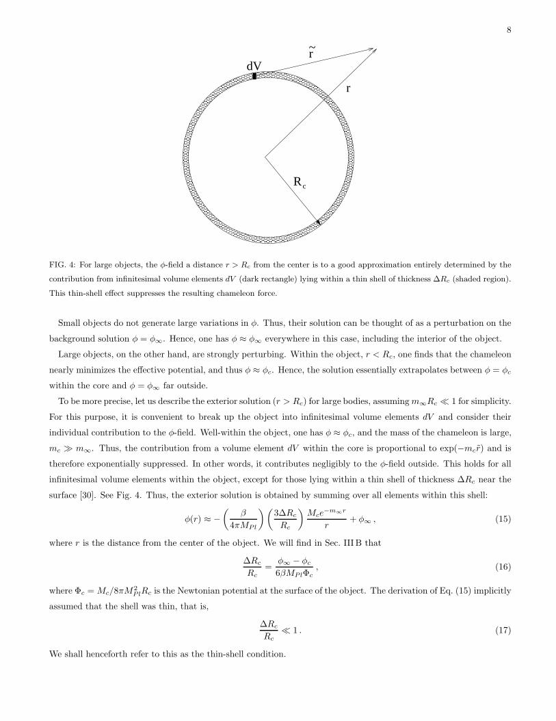
FIG. 4: For large objects, the φ-field a distance r > Rc from the center is to a good approximation entirely determined by the

contribution from infinitesimal volume elements dV (dark rectangle) lying within a thin shell of thickness ∆Rc (shaded region).

This thin-shell effect suppresses the resulting chameleon force.

Small objects do not generate large variations in φ. Thus, their solution can be thought of as a perturbation on the

background solution φ = φ∞. Hence, one has φ ≈ φ∞ everywhere in this case, including the interior of the object.

Large objects, on the other hand, are strongly perturbing. Within the object, r < Rc, one finds that the chameleon

nearly minimizes the effective potential, and thus φ ≈ φc. Hence, the solution essentially extrapolates between φ = φc

within the core and φ = φ∞ far outside.

To be more precise, let us describe the exterior solution (r > Rc) for large bodies, assumingm∞Rc ≪ 1 for simplicity.

For this purpose, it is convenient to break up the object into infinitesimal volume elements dV and consider their

individual contribution to the φ-field. Well-within the object, one has φ ≈ φc, and the mass of the chameleon is large,

mc ≫ m∞. Thus, the contribution from a volume element dV within the core is proportional to exp(−mcr) and is

therefore exponentially suppressed. In other words, it contributes negligibly to the φ-field outside. This holds for all

infinitesimal volume elements within the object, except for those lying within a thin shell of thickness ∆Rc near the

surface [30]. See Fig. 4. Thus, the exterior solution is obtained by summing over all elements within this shell:

φ(r) ≈ −(

β

4πMPl

) (

3∆Rc

Rc

)

Mce−m∞r

r+ φ∞ , (15)

where r is the distance from the center of the object. We will find in Sec. III B that

∆Rc

Rc=

φ∞ − φc

6βMPlΦc, (16)

where Φc = Mc/8πM2PlRc is the Newtonian potential at the surface of the object. The derivation of Eq. (15) implicitly

assumed that the shell was thin, that is,

∆Rc

Rc≪ 1 . (17)

We shall henceforth refer to this as the thin-shell condition.

9

Small objects, in the sense that ∆Rc/Rc > 1, do not have a thin shell. Rather, their entire volume contributes to

the φ-field outside, and thus the exterior solution is

φ(r) ≈ −(

β

4πMPl

)

Mce−m∞r

r+ φ∞ , (18)

which is recognized as the Yukawa profile for a scalar field of mass m∞. Note that Eq. (15) and (18) differ only by a

thin-shell suppression factor of ∆Rc/Rc. To summarize, the exterior solution for a compact object is given by

φ(r) ≈ −(

β

4πMPl

)

Mce−m∞r

r+ φ∞ if

∆Rc

Rc> 1 ;

φ(r) ≈ −(

β

4πMPl

) (

3∆Rc

Rc

)

Mce−m∞r

r+ φ∞ if

∆Rc

Rc≪ 1 , (19)

with ∆Rc/Rc defined in Eq. (16).

The ratio (φ∞ − φc)/MPlΦc, which appears in Eq. (16) and determines whether or not an object has a thin shell,

can be interpreted physically as follows. Given a background profile φ(r), it is straightforward to show from the

action (1) that the resulting chameleon-force on a test particle of mass M and coupling β is given by

~Fφ = − β

MPlM~∇φ . (20)

It follows that φ should be thought of as a potential for this “fifth” force. Thus, (φ∞ − φc)/MPlΦc is the ratio of the

difference in φ potential to the Newtonian potential, and effectively quantifies how perturbing the object is for the φ

field.

B. Derivation

To get an intuition for the boundary value problem at hand, it is useful to think of r as a time coordinate and

φ as the position of a particle, and treat Eq. (11) as a dynamical problem in classical mechanics. This is akin to

the familiar trick performed in bubble nucleation calculations [31]. In this language, the particle moves along the

inverted potential −Veff , and the second term on the left-hand side of Eq. (11), proportional to 1/r, is recognized

as a damping term. An important difference here is that −Veff is “time”-dependent since ρ depends on r. More

precisely, the effective potential undergoes a jump at time r = Rc, as illustrated in Fig. 5.

The particle begins at rest, since dφ/dr = 0 at r = 0, from some initial value which we denote by φi:

φi ≡ φ(r = 0) . (21)

For small r, the friction term is large, and thus the particle is essentially frozen at φ = φi. It remains stuck there

until the damping term, proportional to 1/r, is sufficiently small to allow the driving term, dVeff/dφ, to be effective.

In other words, the amount of “time” the particle remains stuck near φ = φi depends on the slope of the potential,

dVeff/dφ, at φ = φi. Once friction is negligible, the particle begins to roll down the potential. See Fig. 5a).

It rolls down until, at some later time r = Rc, the potential suddenly changes shape as ρ(r) undergoes a jump from

ρc to ρ∞ (see Eq. (12)). But φ and dφ/dr are of course continuous at the jump, and the particle keeps rolling, this

time climbing up the inverted potential. See Fig. 5b). If the initial position φi is carefully chosen, the particle will

barely reach φ∞ in the limit r → ∞, as desired. (It is easy to prove that such φi always exists.) Thus the problem is

reduced to determining the initial value φi.

10

ρc

φ

φ)-V (eff

inf

φ)

φ

ρ

-V (eff

a) r < R c

exp(βφ/ )PlM

b) r > Rc

exp(βφ/ )PlM

FIG. 5: The inverted potential −Veff for a compact object of radius Rc is discontinuous at r = Rc since the matter density

equals: a) ρc for r < Rc; b) ρ∞ for r > Rc. The dots represent the position of the particle at some value of r.

In the end φi will depend on the physical properties of the compact object, such as its density ρc and its radius

Rc, as well as on the various parameters of the theory, such as β and the shape of the potential. Rather than first

choosing a set of values for ρc, Rc, etc. and then solving for φi, we will instead choose a range of φi and determine

the corresponding region in the (ρc, Rc, . . .) parameter space. More precisely, we shall consider the two regimes

(φi − φc) ≪ φc and φi ∼> φc, and we will show that these correspond respectively to ∆Rc/Rc ≪ 1 and ∆Rc/Rc > 1.

Anticipating this result, we refer to these two regimes as thin-shell and thick-shell, respectively.

Thin-shell regime: (φi − φc) ≪ φc. This corresponds to φ being released from a point very close to φc. Since φc

is a local extremum of the effective potential, the driving term dVeff/dφ is negligible initially, and the dynamics are

strongly dominated by friction. Consequently, the field remains frozen at its initial value φi ≈ φc for a long time,

until the friction force is sufficiently small to allow the particle to roll. We shall denote by Rroll the “moment” at

which this occurs. Hence, we have

φ(r) ≈ φc for 0 < r < Rroll . (22)

When r ∼ Rroll, the field is still near φc but has now begun to roll. Since MPl|V,φ| ≪ βρeβφ/MP l as soon as φ is

displaced significantly from φc, as illustrated in Fig. 2, we may approximate Eq. (11) in the regime Rroll < r < Rc

by

d2φ

dr2+

2

r

dφ

dr≈ β

MPlρc , (23)

where we have also assumed βφ/MPl ≪ 1. The solution to Eq. (23) with boundary conditions φ = φc and dφ/dr = 0

at r = Rroll is

φ(r) =βρc

3MPl

(

r2

2+R3

roll

r

)

− βρcR2roll

2MPl+ φc for Rroll < r < Rc . (24)

The full solution for 0 < r < Rc is thus approximated by Eqs. (22) and (24). The approximation of separating the

solution into the two regions 0 < r < Rroll and Rroll < r < Rc only makes sense, however, if Rc − Rroll ≪ Rc. For

11

otherwise there is no clear separation between the two regions, and one needs a solution valid over the entire range

0 < r < Rc.

At r = Rc, the energy density undergoes a jump from ρc to ρ∞, as described by Eq. (12). For r > Rc, the effective

potential is shown in Fig. 5 b), and the particle is climbing up the hill. Since the speed of the particle is initially large

compared to the curvature of the potential, Eq. (11) can be approximated by

d2φ

dr2+

2

r

dφ

dr≈ 0 , (25)

whose solution, satisfying φ→ φ∞ as r → ∞, is given by

φ(r) ≈ −Ce−m∞(r−Rc)

r+ φ∞ , (26)

where C is a constant and where we have used the fact that the potential is approximately quadratic near φ = φ∞.

The two unknowns, Rroll and C, are then determined by matching φ and dφ/dr at r = Rc using Eqs. (24) and (26).

With the approximation that Rc −Rroll ≪ Rc, it is straightforward to show that the exterior solution is

φ(r) ≈ −(

β

4πMPl

) (

3∆Rc

Rc

)

Mce−m∞(r−Rc)

r+ φ∞ , (27)

with

∆Rc

Rc≡ φ∞ − φc

6βMPlΦc≈ Rc −Rroll

Rc≪ 1 , (28)

where we have substituted the Newtonian potential Φc.

Thick-shell regime: φi ∼> φc. In this case, the field is initially sufficiently displaced from φc that it begins to roll

almost as soon as it is released at r = 0. Hence there is no friction-dominated regime in this case, and the interior

solution for φ is most easily obtained by taking the Rroll → 0 limit of Eq. (24) and replacing φc by φi. Matching to

the exterior solution as before, we obtain

φ(r) =βρcr

2

6MPl+ φi for 0 < r < Rc (29)

and

φ(r) ≈ −(

β

4πMPl

)

Mce−m∞(r−Rc)

r+ φ∞ for r > Rc . (30)

Moreover, equating these two equations at r = Rc, we find φi = φ∞ − 3βΦc/MPl. In particular, since φi ∼> φc and

using the definition ∆Rc/Rc = (φ∞ − φc)/6βMPlΦc, this implies

∆Rc

Rc> 1 . (31)

We conclude this Section with a word on how the above solutions, which assumed homogeneous ρ, can be generalized

to the more realistic case of spatially-varying matter density. In most cases of interest, such as the interior of the

Earth for instance, we will find that the matter density varies on scales much larger than the Compton wavelength

m−1 of the chameleon field in that region. More precisely, it is generally the case that |∇ log ρ(~x)| ≪ m within dense

objects. If so, one can make an adiabatic approximation which consists of treating ρ(~x) as a constant in the equations

of motion. In other words, in this case one may simply substitute ρ(~x) in the expressions above.

12

IV. PROFILE FOR THE EARTH

Since the most stringent constraints on possible violations of the EP derive from experiments performed on Earth, it

is important to discuss in some detail the profile for φ inside and in the vicinity of the Earth. Admittedly, the model

for our planet described below is rather crude, but is sufficiently accurate to derive order-of-magnitude estimates

of resulting violations of the EP. More realistic descriptions can be obtained for instance by using the adiabatic

approximation discussed at the end of Sec. III, or through numerical analysis.

The Earth is modeled as a solid sphere of radius R⊕ = 6 · 108 cm and homogeneous density ρ⊕ = 10 g/cm3.

Surrounding it is an atmosphere which we approximate as a layer 10 km in radius with homogeneous density ρatm =

10−3 g/cm3. Moreover, we treat our planet as an isolated body, neglecting the effect of surrounding compact objects

such as the Sun and the Moon. Furthermore, far away from the Earth, the matter density is approximated by the

density of homogeneous gas and dark matter in our local neighborhood of the galaxy: ρG = 10−24 g/cm3.

The set-up is thus almost identical to that of Eq. (11), except that the matter density now has three phases instead

of two:

ρ(r) =

ρ⊕ for 0 < r < R⊕

ρatm for R⊕ < r < Ratm

ρG for r > Ratm

, (32)

where Ratm ≡ R⊕+ 10 km. We henceforth denote by φ⊕, φatm and φG the field value which minimizes the effective

potential for the respective densities. Similarly, m⊕, matm and mG are the respective masses.

Following the discussion in Sec. III, the solution depends on whether or not the Earth and its atmosphere have a

thin shell. As we will prove below, it is necessary that the atmosphere has a thin shell, for otherwise unacceptably

large violations of the EP will ensue. In this case, one has φ ≈ φatm in the bulk of the atmosphere. Moreover, since

the Earth is much denser than the atmosphere, it follows that the Earth itself has a thin shell, in which case φ ≈ φ⊕

inside the Earth.

From Eqs. (16) and (17), the thin-shell condition for the atmosphere reads

∆Ratm

Ratm=

φG − φatm

6βMPlΦatm≪ 1 , (33)

where Φatm ≡ ρatmR2atm/6M

2Pl. We can refine this bound by noting that, in order for the atmosphere to have a thin

shell, clearly the thickness of the shell must be less than the thickness of the atmosphere itself, which is ≈ 10−3Ratm.

Hence this requires ∆Ratm/Ratm ∼< 10−3. Using the fact that ρatm ≈ 10−4ρ⊕, and thus Φatm ≈ 10−4Φ⊕, we can

write this as

∆R⊕

R⊕

≡ φG − φatm

6βMPlΦ⊕

< 10−7 . (34)

This condition, which ensures that the atmosphere has a thin shell, will play a crucial role in the analysis of tests

of gravity in the following sections. The exterior solution, r > Ratm, is then given by Eq. (27) with m∞ = mG and

φ∞ = φG:

φ(r) ≈ −(

β

4πMPl

) (

3∆R⊕

R⊕

)

M⊕e−mG(r−Ratm)

r+ φG . (35)

13

To summarize, the solution for φ for the Earth and its atmosphere is well-approximated by

φ(r) ≈ φ⊕ for 0 < r ∼< R⊕ ;

φ(r) ≈ φatm for R⊕ ∼< r ∼< Ratm ;

φ(r) ≈ −(

β

4πMPl

) (

3∆R⊕

R⊕

)

M⊕e−mG(r−Ratm)

r+ φG for r ∼> Ratm , (36)

where ∆R⊕/R⊕ is defined in Eq. (34).

It remains to show that tests of the EP require the atmosphere to have a thin shell. The proof proceeds by

contradiction. Suppose that condition (34) is violated and instead we have

∆R⊕

R⊕

> 10−7 . (37)

We can therefore ignore the atmosphere altogether, and thus the φ-profile in the laboratory is given by Eq. (35):

φ(r) ≈ −(

β

4πMPl

) (

3∆R⊕

R⊕

)

M⊕

r+ φG for r ∼> R⊕ , (38)

where we have neglected the exponential factor since mGR⊕ ≪ 1, as we will see in Sec. VI. From Eq. (20), this profile

results in a fifth force on a test particle of mass M and coupling βi of magnitude

|~Fφ| = 2ββi

(

3∆R⊕

R⊕

)

M⊕M

8πM2Plr

2. (39)

Supposing that the βi’s are all of order β but assume different values for different matter species, then the resulting

difference in relative free-fall acceleration for two bodies of different composition will be

η ≡ 2|a1 − a2|a1 + a2

∼ 10−4β2 ∆R⊕

R⊕

, (40)

where η is the Eotvos parameter, and where the numerical coefficient is appropriate for Cu and Be test masses [10],

as used in the Eot-Wash experiment [9]. For β of order unity, we see from Eq. (37) that this violates the bound

η < 10−13. It follows that the atmosphere must be have a thin shell.

V. SEARCHES FOR EP VIOLATION AND FIFTH FORCE ON EARTH

The tightest constraints on our model derive from laboratory tests of the EP and searches for a fifth force [8, 17].

Since these experiments are usually done in vacuum, we first need to derive an approximate solution for the chameleon

inside a vacuum chamber. For simplicity, we model the chamber as a perfectly empty, spherical cavity of radius Rvac.

In the absence of any other parts within the chamber, and ignoring the effect of the walls, the equation for φ is given

by Eq. (11):

d2φ

dr2+

2

r

dφ

dr= V,φ +

β

MPlρ(r) , (41)

where we have assumed βφ/MPl ≪ 1 as we did throughout Sec. III, and where

ρ(r) ≈

0 for r < Rvac

ρatm for r > Rvac

. (42)

14

The boundary conditions are the same as in Sec. III: dφ/dr = 0 at r = 0 and φ→ φatm as r → ∞.

The solution within the vacuum chamber is analogous to the solution for a compact object with thin-shell (see

Sec. III). In both cases, due to the large density contrast between the object or the vacuum cavity and their

environment, φ must start at r = 0 from a point where it can remain almost frozen for the entire volume. That is,

for 0 < r < Rc in the case of the overdense object and 0 < r < Rvac for the vacuum cavity. For a compact object,

this freezing point lies naturally near the local extremum φ = φc of the effective potential. For the vacuum chamber,

the effective potential has no extremum for r < Rvac (since ρ = 0 there), and thus the only way φ can remain still is

by starting from a point where it will be friction-dominated for almost the entire range 0 < r < Rvac. In other words

the curvature of the potential at that point must be of order R−2vac, that is, this freezing point corresponds to a value

φ = φvac where the mass of small fluctuations, mvac, is equal to R−1vac.

While the precise solution to (41) depends of course on the details of the potential, numerical analysis confirms the

above qualitative discussion:

• The chameleon assumes the value φ ∼ φvac within the vacuum chamber, where φvac satisfies

mvac ≡√

V,φφ(φvac) = R−1vac . (43)

That is, φvac is the field value about which the Compton wavelength of small fluctuations equals Rvac, the

radius of the chamber.

• Throughout the chamber, φ varies slowly, with |dφ/dr| ∼< φvac/Rvac.

• Outside the chamber the solution tends to φatm within a distance of m−1atm from the walls.

These generic properties are all we need for our analysis.

A. Fifth Force Searches

The potential energy associated with fifth force interactions is generally parameterized by a Yukawa potential:

V (r) = −αM1M2

8πM2Pl

e−r/λ

r, (44)

where M1 and M2 are the masses of two test bodies, r is their separation, α is the strength of the interaction (with

α = 1 for gravitational strength), and λ is the range. Null fifth-force searches therefore constrain regions in the (λ, α)

parameter space (see Fig. 2.13 of [17]).

As discussed above, the range λ of φ-mediated interactions inside a vacuum chamber is of the order of the size of

the chamber. That is, λ ≈ Rvac. For λ ≈ 10 cm−1 m, the tightest bound on the coupling constant α from laboratory

experiments is from Hoskins et al. [32]:

α < 10−3 . (45)

Now consider two identical test bodies of uniform density ρc, radius Rc and total mass Mc. If these have no thin

shell, then they each generate a field profile given by Eq. (18) with φ∞ = φvac and m∞ = R−1vac:

φ(r) ≈ −(

β

4π

)

Mc

MPl

e−r/Rvac

r+ φvac . (46)

15

Dropping the irrelevant constant, the resulting potential energy is

V (r) = −2β2 M2c

8πM2Pl

e−r/Rvac

r. (47)

Comparison with Eq. (44) shows that the coupling strength is α = 2β2 in this case, which clearly violates the bound

in Eq. (45) for β ∼ O(1).

Hence it must be that the test masses have a thin shell, that is,

∆Rc

Rc≡ φvac − φc

6βMPlΦc≪ 1 . (48)

In this case, their field profile is given by Eq. (15):

φ(r) ≈ −(

β

4πMPl

) (

3∆Rc

Rc

)

Mce−r/Rvac

r+ φvac , (49)

and the corresponding potential energy is

V (r) = −2β2

(

3∆Rc

Rc

)2M2

c

8πM2Pl

e−r/Rvac

r. (50)

Once again comparing with Eq. (44), we find that the bound in Eq. (45) translates into

2β2

(

3∆Rc

Rc

)2

∼< 10−3 . (51)

Note that, β ∼> O(1), this constraint implies that the thin-shell condition in Eq. (48) is satisfied.

To make the condition (51) more explicit, note that a typical test body used in Hoskins et al. had mass Mc ≈ 40 g

and radius Rc ≈ 1 cm, corresponding to Φc ≈ 3 · 10−27. Substituting in Eq. (48) and assuming φvac ≫ φc, we obtain

the constraint

φvac ∼< 10−28 MPl , (52)

which ensures that the current bounds from laboratory searches of a fifth force are satisfied.

B. Tests of the EP

Turning our attention to the magnitude of EP violations inside our vacuum cavity, we recall that the solution for

φ inside the chamber satisfies∣

∣

∣

∣

dφ

dr

∣

∣

∣

∣ ∼<φvac

Rvac. (53)

From Eq. (20), this yields an extra component to the acceleration of magnitude (β/MPl)φvac/Rvac. For Cu and Be

test masses, as used in the Eot-Wash experiment [9], this yields an Eotvos parameter of

η ∼ 4π10−4βMPlR

2⊕

M⊕

φvac

Rvac. (54)

Substituting Rvac = 10 cm and β ∼ O(1), the Eot-Wash constraint of η < 10−13 translates into

φvac ∼< 10−26 MPl , (55)

which is a much weaker constraint than Eq. (52) and thus shall henceforth be ignored.

16

VI. RESULTING CONSTRAINTS ON MODEL PARAMETERS

In this Section we summarize the constraints derived in the previous sections and apply them to a general power-law

potential

V (φ) = M4+nφ−n , (56)

where M has units of mass and n is a positive constant. As mentioned earlier, potentials of this form have the desired

features for quintessence models of the universe [27]. We will find that the energy scale M is generally constrained

to be of the order of (1 mm)−1. We then discuss the resulting bounds on the interaction range in the atmosphere, in

the solar system and on cosmological scales.

Broad considerations of EP violation lead us to conclude in Sec. IV that both the Earth and its atmosphere must

have a thin shell. This resulted in the constraint (see Eq. (34)):

∆R⊕

R⊕

≡ φG − φatm

6βMPlΦ⊕

< 10−7 . (57)

Recall that, by definition, φG is the value of φ which minimizes the effective potential with ρ = ρG, i.e., V,φ(φG) +

βρGeβφG/MP l/MPl = 0. Assuming βφG/MPl ≪ 1 and substituting the power-law potential of Eq. (56) gives

φG =

(

nM4+nMPl

βρG

)1/(n+1)

. (58)

With ρG = 10−24 g/cm3 and Φ⊕ = 10−9, it is then straightforward to show that Eq. (57) can be rewritten as a bound

on M :

M <

(

6n+1

n

)1

n+4

βn+2

n+4 · 1015n−7

n+4 · (1 mm)−1 . (59)

Then, in Sec. V, we studied laboratory tests of the EP and fifth force, including the fact that these are performed

in vacuum, and derived the condition

φvac ∼< 10−28 MPl , (60)

where φvac is the field value about which the Compton wavelength of small fluctuations is of the order of the size of

the vacuum chamber, Rvac. Applying Eq. (43) to the power-law potential yields

R−2vac = 10−68 M2

Pl = n(n+ 1)M4+nφ−(n+2)vac , (61)

where we have assumed Rvac = 1 m = 1034 M−1Pl for concreteness. It is easy to see that smaller values of Rvac result

in weaker constraints, and this is therefore a conservative choice. It is then straightforward to show that Eq. (52)

reduces

M ∼< [n(n+ 1)]−1/(4+n) · 103n/(4+n) · (1 mm)−1 . (62)

We thus see that, for n and β of order unity, Eqs. (59) and (62) both constrain M to be less than approximately

an inverse millimeter, or 10−3 eV. It is remarkable that this is also the mass scale associated with the cosmological

constant or dark energy causing the present acceleration of the universe [24]. Granted, this is tiny compared to typical

17

particle physics scales, such as the weak or the Planck scale, and thus our potential (56) suffers from fine-tuning.

Nevertheless, it is our hope that whatever mechanism suppresses the scale of the cosmological constant from its natural

value of 1018 GeV down to 10−3 eV might also naturally account for the energy scale characterizing our potential.

The above constraints can be translated into bounds on the range of chameleon-mediated interactions in the

atmosphere (m−1atm), in the solar system (m−1

G ) and on cosmological scales today (m−10 ). From Eq. (10), these are

given by

m2atm = V,φφ(φatm) +

β2

M2Pl

ρatmeβφatm/MP l

m2G = V,φφ(φG) +

β2

M2Pl

ρGeβφG/MP l

m20 = V,φφ(φ0) +

β2

M2Pl

ρ0eβφ0/MP l , (63)

where ρ0 ≈ 10−29 g/cm3 is the current energy density of the universe and φ0 is the corresponding value of φ on

cosmological scales. Substituting the above bounds on M , it is straightforward to show that, for n ∼< 2 and β of order

unity,

m−1atm ∼< 1 mm − 1 cm

m−1G ∼< 10 − 104 AU

m−10 ∼< 0.1 − 103 pc , (64)

where the numbers on the right-hand depend somewhat on the value of n and β (recall that 1 AU ≈ 1.5 · 1013 cm and

1 pc ≈ 3 · 1018 cm).

Thus, while φ-interactions are short-range in the atmosphere (short compared to the size of the atmosphere), they

are rather long-range in the solar system. In particular, it is possible for the scalar field to be essentially free on solar

system scales. This striking difference in behavior of the field in space compared to Earth is an original ingredient of

our scenario and, as we will show in Sec. IX, can lead to unexpectedly large signals for EP and fifth force experiments

to be performed in orbit in the near future. On cosmological scales, we see that a power-law potential implies an

interaction range which is smaller than the present size of the observable universe, H−10 ∼ 109 pc. It follows that m0

is too large for φ to be rolling on cosmological time scales today. A general study of potentials and their viability for

quintessence models of the universe will be presented in a future paper [24].

VII. SOLAR SYSTEM TESTS OF GRAVITY

In this Section, we discuss the constraints on scalar-tensor theories from planetary orbits, in particular from solar

system tests of the EP and fifth force (Sec. VII A), as well as post-Newtonian corrections (Sec. VII B). In short, these

constraints are all satisfied because large bodies, such as the Sun and the Earth, all have a thin shell which greatly

suppresses the φ-force between them.

18

A. Solar System Tests of EP and Fifth Force

Precise measurements of the lunar orbit from laser ranging constrains the difference in free-fall acceleration of the

Moon and the Earth towards the Sun to be less than approximately one part in 1013 [8]. That is, denoting their

respective acceleration by aMoon and a⊕, we have

|aMoon − a⊕|aN

∼< 10−13 , (65)

where aN is the Newtonian acceleration.

In our model, this difference is naturally very small since the Sun, Earth and Moon are all subject to the thin shell

effect. We have already imposed that the Earth (and its atmosphere) have a thin shell. So must the Sun, therefore,

since its Newtonian potential is larger than that of the Earth. Hence we only need to show that the same holds true

for the Moon. But, assuming φG ≫ φMoon, this trivially follows from Eq. (34):

∆RMoon

RMoon∼ ∆R⊕

R⊕

Φ⊕

ΦMoon< 10−5 , (66)

where we have used Φ⊕ = 10−9 and ΦMoon = 10−11.

Hence the φ profile outside each of these bodies is given by Eq. (27) with m∞ = mG and φ∞ = φG. Assuming

m−1G > 1 AU, since this yields maximal violation of the EP, it is then straightforward to show that the acceleration

of the Earth towards the Sun is given by

a⊕ = aN ·{

1 + 18β2

(

∆R⊕

R⊕

) (

∆R⊙

R⊙

)}

≈ aN ·{

1 + 18β2

(

∆R⊕

R⊕

)2Φ⊕

Φ⊙

}

, (67)

while for the Moon

aMoon = aN ·{

1 + 18β2

(

∆RMoon

RMoon

) (

∆R⊙

R⊙

)}

≈ aN ·{

1 + 18β2

(

∆R⊕

R⊕

)2 Φ2⊕

Φ⊙ΦMoon

}

. (68)

Substituting Φ⊙ = 10−6, Φ⊕ = 10−9 and ΦMoon = 10−11, this gives a difference in free-fall acceleration of

|aMoon − a⊕|aN

≈ β2

(

∆R⊕

R⊕

)2

< β2 · 10−14 , (69)

where we have used Eq. (34) in the last step. This satisfies the bound in Eq. (65) for reasonable values of β.

We next consider solar-system tests of the existence of a fifth force. Deviations from a 1/r2 force law, for instance

due to the exponential factor in Eq. (44), contribute an anomalous component to the perihelion precession of planetary

orbits in comparison with the predictions of GR. For instance, Lunar laser-ranging measurements lead to the constraint

α ∼< 10−10 for a fifth-force with range λ ∼ 108 m [34]. A similar analysis for the orbits of Mercury and Mars gives

α ∼< 10−9 for the range λ ∼ 1 AU [35]. (Not surprisingly, these tests are most sensitive to a fifth force whose range is of

the order of the distance between the Sun and the orbiting body.) In our model, these celestial objects are all subject

to the thin-shell effect, and, just as with the EP analysis above, the screening mechanism makes the constraints from

perihelion precession trivial to satisfy.

19

B. Tests of Post-Newtonian Gravity

To estimate the constraints from post-Newtonian corrections, consider the φ-profile due to the Earth given by

Eq. (35):

φ(r) ≈ −(

β

4πMPl

) (

3∆R⊕

R⊕

)

M⊕

r+ φG , (70)

where we have neglected the exponential factor. Comparison with the expected profile if there were no thin-shell

suppression, given by Eq. (30), we see that the exterior solution above corresponds to that of a massless scalar with

effective coupling

βeff = 3β∆R⊕

R⊕

< 3β · 10−7 , (71)

where in the last step we have used the condition that the atmosphere has a thin-shell (see Eq. (34)). Treating our

model as a Brans-Dicke theory with effective coupling constant βeff given above, which is a good approximation

in the solar system since the chameleon behaves essentially as a free field, it is straightforward to show that the

corresponding effective Brans-Dicke parameter, ωBD, is given by [8]

3 + 2ωBD =1

2β2eff

∼> 6 · 1012β−2 . (72)

The tightest constraint on Brans-Dicke theories comes from light-deflection measurements using very-long-baseline

radio interferometer [8]: ωBD > 3500. We see that this is easily satisfied in our model. Similarly, one can show that

the constraint from the decay of the orbital period of binary pulsars, ωBD > 100, is trivially satisfied. (Note that

density-dependent effective couplings were previously noted in a different context [33].)

VIII. TESTS OF THE STRONG EP

Our discussion of the EP has so far been restricted to the weak EP, which essentially states that the laws of gravity

are the same in any inertial frame. General Relativity, however, satisfies a stronger version of the EP [8], in the sense

that all laws of physics, including non-gravitational interactions, assume the same form in any inertial frame (local

Lorentz invariance), and the various parameters describing these non-gravitational forces, such as the fine-structure

constant, are independent of space and time (local position invariance).

At any space-time event, one can find a coordinate system in which the Einstein-frame metric gµν equals the

Minkowski metric ηµν . Since all other metrics g(i)µν appearing in the action (1) are conformally-related to gµν , all g

(i)µν

are proportional to ηµν in this frame. All laws of physics are therefore Lorentz invariant at that space-time event,

and thus our model satisfies local Lorentz invariance.

The most stringent constraint on spatial variations of couplings comes from the Vessot-Levine experiment [23] which

measured the redshift between a hydrogen-maser clock flown at an altitude of 104 km and another one on the ground.

In a theory which has LPI, as in GR, the redshift z is given by the difference in Newtonian potential ∆Φ between the

emitter and the receiver [36]. As shown in Will [8], LPI violations generate an extra contribution ∆z to the redshift,

of the form

∆z = γ · ∆Φ , (73)

20

where γ is a constant that depends on the Newtonian potential of the emitter, with γ = 0 corresponding to the case

of no LPI violation. The bound from the Vessot-Levine experiment is |γ| ∼< 10−4.

To estimate γ in our case, recall from Eq. (2) that a test particle of the matter field ψ(i)m follows geodesics of the

metric g(i)µν related to the Einstein-frame metric gµν by g

(i)µν = e2βiφ/MP lgµν . Thus, a constant mass scale m(i) in

the ψ(i)m -frame is related to a φ-dependent mass scale m(φ) in Einstein frame by the rescaling m(φ) = eβiφ/MP lm(i).

Similarly, a ψ(i)m -clock with frequency ν(i) is measured in Einstein frame to have a frequency ν(φ) = eβiφ/MP lν(i).

Assuming βφ/MPl ≪ 1, the φ-dependence of ν therefore yields the following extra contribution to the redshift:

∆z ≈ − β

MPl(φ(rem) − φ(rrec)) , (74)

where we have dropped the superscript (i), and where rem (rrec) is the distance between the emitter (receiver) and

the center of the Earth. For the Vessot-Levine experiment, we have rem ≈ 104 km ≈ 2R⊕ and rrec ∼> R⊕, and it

follows from Eqs. (36) that φ(rem) ≈ φG and φ(rrec) ≈ φatm, respectively. Since ∆Φ ≈ Φ⊕/2 in this case, massaging

Eq. (74) gives

∆z = −12β2

(

φG − φatm

6βMPlΦ⊕

)

∆Φ , (75)

from which we can read off the corresponding value of γ:

|γ| = 12β2 ∆R⊕

R⊕∼< β2 · 10−6 . (76)

This comfortably satisfies the Vessot-Levine bound of |γ| ∼< 10−4.

Time-variation of coupling constants are constrained by geophysical measurements (such as the Oklo Nuclear

Reactor [37]), by the study of absorption lines in quasar spectra and by nucleosynthesis. Recent analysis indicates

that the fine-structure constant has evolved by more than one part in 105 over the cosmological redshift range

0.2 < z < 3.7 [5], thus suggesting that LPI does not hold in the Universe.

In our scenario, the various coupling constants are determined by φ, whose value depends on the local density.

Thus, even though the coupling constants may vary on cosmological scales today, the fact that the density of the

Earth is constant in time implies that the various couplings measured on Earth do not vary significantly. In particular,

this implies that constraints from the Oklo Nuclear Reactor are easily evaded in our model. (See [38] for a related

discussion of a density-dependent fine-structure constant.)

In any case, we find that the time-variation of coupling constants and masses on cosmological scales is very small

in the case of the power-law potential of Eq. (56). To see this, consider once again a constant mass scale m(i) in

the matter frame, with corresponding m(φ) = eβiφ/MP lm(i) in the Einstein frame. Hence, the time variation of m(φ)

between nucleosynthesis and the present epoch, say, is given by∣

∣

∣

∣

∆m

m

∣

∣

∣

∣

≈ β

MPl(φ0 − φBBN ) , (77)

where φBBN is the value of φ at nucleosynthesis. For the power-law potential considered earlier, V (φ) = M4+nφ−n,

the bound of M ∼< (1 mm)−1 derived in Sec. VI gives∣

∣

∣

∣

∆m

m

∣

∣

∣

∣ ∼< β · 10−11 , (78)

which satisfies all current astrophysical and cosmological bounds. In particular, it appears that the power-law potential

cannot account for the variation of the fine-structure constant reported by Webb et al. [5]. A more detailed analysis of

time-variation of coupling constants in our model, including more general potentials, will be presented elsewhere [24].

21

IX. NEW PREDICTIONS FOR NEAR-FUTURE SATELLITE EXPERIMENTS

Our scenario has the remarkable feature that the physical characteristics of the scalar field can be very different in

the laboratory than in space. We have seen, for instance, that the range of the interactions it mediates is of order

1 mm in the atmosphere while being greater than 10 AU in the solar system. Hence, as we will show in this Section,

the predicted strength of EP violations and fifth force can be strikingly different in orbit than in the laboratory. This

is particularly interesting as this decade should witness the launch of several satellite experiments that aim at making

these measurements. Three of them, namely STEP, GG and MICROSCOPE, will test the universality of free-fall

with respective expected sensitivity of 10−18, 10−17 and 10−15 for the Eotvos parameter η. Another satellite, the SEE

Project, will further attempt to measure a fifth force between two test bodies in orbit.

In this Section we will show that, for a wide range of parameters, our model predicts that these satellite experiments

will see a strong signal. It is in fact likely that the signal will be stronger than previously thought possible based on

laboratory measurements. For instance, the SEE capsule could detect corrections to the effective Newton’s constant

(including fifth force contribution) of order unity compared to the value measured on Earth or inferred from planetary

motion. Moreover, STEP, GG and MICROSCOPE could measure violations of the EP with η > 10−13, which is larger

than the current bound from the (ground-based) Eot-Wash experiment. Such outcomes would constitute a smoking

gun for our model, for it would otherwise be difficult to reconcile the results in space with those on Earth.

Let us begin with the SEE satellite, which will orbit the Earth at an altitude of approximately 103 km. This multi-

faceted experiment will test for deviations from 1/r2 in the force law, search for violations of the EP and measure

Newton’s constant G to one part in 107. This will be achieved by accurately determining the orbit of two tests masses

as they interact gravitationally with each other and with the Earth. For our purposes we shall focus on the expected

value of G, including the contribution from the fifth force mediated by φ.

We first show that it is possible for the satellite not to have a thin shell. This is desirable in this case in order to

maximize the signal. That is, we derive the conditions under which ∆RSEE/RSEE > 1 holds for the SEE capsule.

According to the current design, the satellite will have a total mass of ∼ 2000 kg and an effective radius of RSEE ∼ 2 m

(although it has cylindrical symmetry, we approximate the capsule as a sphere of equal volume for simplicity). Thus

its Newtonian potential is ΦSEE ≈ 10−24 ≈ 10−15Φ⊕. Moreover, at an altitude of 1000 km, the chameleon field

assumes the value φ(rSEE) ∼ φG, as seen from Eq. (35). Therefore, the condition ∆RSEE/RSEE > 1 requires

∆R⊕

R⊕

> 10−15 . (79)

Combining this with the condition that the atmosphere have a thin shell, Eq. (57), we find that the allowed range for

which the SEE satellite will not have a thin shell is

10−15 <∆R⊕

R⊕

< 10−7 . (80)

This constitutes a wide region in parameter space. Following the analysis of Sec. VI, for a potential V (φ) = M4+nφ−n

with n = 1/3 and β = 10, this requires the range of interactions in the atmosphere, m−1atm, to be anywhere between

0.1 µm and 1 mm.

Therefore, if the inequality in Eq. (79) is satisfied, the scalar field φ is only slightly perturbed by the satellite, and

thus the field value within the capsule is φ ∼ φG. Moreover, since m−1G is much larger than the size of the satellite, φ

22

behaves as a massless field. Hence, if the test bodies have mass Mi and coupling βi, i = 1, 2, they will experience a

total force, gravitational plus φ-mediated, given by

|~F | =GM1M2

r2(1 + 2β1β2) , (81)

where we have restored Newton’s constant G = (8πM2Pl)

−1. This implies, therefore, that the SEE satellite will

measure an effective Newton’s constant, Geff ≡ G(1 + 2β1β2), which differs by order unity from Newton’s constant

measured on Earth.

Since this is an important prediction, let us summarize how it was obtained. First of all, the key ingredient is that

the SEE experiment is performed in orbit, where the range of φ-mediated interactions is greater than 10 AU. Thus,

small perturbations in φ are essentially massless on the scale of the capsule, and therefore the force law between

two test bodies is proportional to 1/r2 to a very good approximation. A second crucial condition is that there is no

thin-shell effect within the satellite, as expressed in Eq. (79). This ensures that there is no suppression of the fifth

force, and the coupling strength is therefore of order β2. Hence, for β of order unity, the effective Newton’s constant

receives large corrections from the fifth force mediated by φ. As mentioned earlier, such an outcome would constitute

strong evidence that a mechanism of the kind we are proposing is at play in Nature.

Our model also has surprising implications for satellite experiments that aim at measuring EP violations in orbit,

such as MICROSCOPE, GG and STEP. These experiments will attempt to measure a difference in free-fall acceleration

between two concentric cylinders of different composition with expected sensitivity of one part in 1015, 1017 and 1018,

respectively.

We focus on the STEP satellite for concreteness. Although Eq. (79) pertains to the SEE capsule, a similar condition

is obtained for STEP, since its physical characteristics are not too different from those of SEE. Hence, there is no

thin-shell effect if Eq. (79) holds, and the φ profile within the satellite is well-approximated by Eq. (35). It is then

straightforward to show that the Eotvos parameter for Be and Nb test cylinders, as appropriate for STEP, is given

by

η ≈ 10−4β2 ∆R⊕

R⊕

. (82)

Combining with Eq. (80), we find the allowed range

β2 · 10−19 < η < β2 · 10−11 , (83)

which falls almost entirely within the range of sensitivity of STEP. Moreover, we see that β can be larger than 10−13,

the current bound from experiments performed on Earth [9]. In other words, it is possible that MICROSCOPE, GG

and STEP will measure violations of EP stronger than currently thought to be allowed by laboratory measurements.

This is another striking manifestation of the fact that scalar field dynamics in our model are very different on Earth

than in orbit.

X. DISCUSSION

In this paper, we have presented a novel scenario in which both the strength and the range of interactions mediated

by a scalar field φ depend sensitively on the surrounding environment. In a region of high density, such as on Earth,

23

the mass of the scalar field is sufficiently large, typically of order 1 mm−1, to evade constraints on EP violation from

laboratory experiments. Meanwhile, the field can be essentially free on solar system scales, with a typical Compton

wavelength of 100 AU.

We have argued that our scenario satisfies all existing bounds from ground-based and solar-system tests of gravity.

It will be left for future work to study our model in the context of strongly gravitating systems, such as black holes [40].

Implications for cosmology will be analyzed in a separate paper [24], where we will show in detail that chameleons are

consistent with cosmological constraints on the existence of non-minimally coupled scalars, such as the bound on the

time-variation of G from nucleosynthesis, for example. Moreover, we will describe how the field dynamically reaches

the minimum of the effective potential, an element that was assumed a priori in the present work, and show how our

scenario naturally provides a solution to the old moduli problem [41].

The striking difference in interaction range in the solar system versus on Earth can lead to unexpected outcomes

for experiments that test gravity in space. It was argued that the SEE Project could measure an effective Newton’s

constant drastically different than that on Earth. Meanwhile, the MICROSCOPE, GG and STEP satellites could

detect violations of the EP stronger than currently allowed by ground-based experiments. Either outcome would

effectively constitute a proof of the existence of chameleons. More importantly, these possible surprises for space

experiments will hopefully strengthen the case for launching these satellites.

Also, the door is open for conceiving of new table-top experiments to probe for the existence of chameleons, for

instance by exploiting the fact that the properties of chameleons are sensitive to the surrounding matter density. For

example, one could imagine doing atomic physics experiments inside or in the vicinity of a massive oscillating shell of

matter. These oscillations would induce a time-dependence in the profile of the chameleon and thus in the frequency

of emission lines [42]. It would also be interesting to investigate the behavior of the field at intermediate altitude,

for instance at about 40 km where balloon experiments take place. This would require a more realistic modeling of

the atmosphere than presented here. Such an analysis could reveal that it may be possible to detect chameleons by

performing gravity experiments in balloons [43].

We thank N. Arkani-Hamed, J.R. Bond, R. Brandenberger, P. Brax, C. van de Bruck, S. Carroll, T. Damour, A.-C.

Davis, G. Esposito-Farese, G. Gibbons, B. Greene, D. Kabat, A. Lukas, J. Murugan, B.A. Ovrut, M. Parikh, S.-J. Rey,

K. Schaalm, C.L. Steinhardt, N. Turok, C.M. Will, T. Wiseman, and especially N. Kaloper and P.J. Steinhardt for

insightful discussions. This work was supported by the Columbia University Academic Quality Fund, the Ohrstrom

Foundation (JK), DOE grant DE-FG02-92ER40699 and the University of Cape Town (AW).

[1] A. Riess et al., AJ 116, 1009 (1998); S. Perlmutter et al., ApJ 517, 565 (1999).

[2] D. Spergel et al., ApJ Supp. 148, 175 (2003).

[3] B. Ratra and P.J.E. Peebles, Phys. Rev. D 37, 3406 (1998).

[4] R.R. Caldwell, R. Dave and P.J. Steinhardt, Phys. Rev. Lett. 80, 1582 (1998); for a review, see J.P. Ostriker and P.J.

Steinhardt, Sci. Am., Jan. issue (2001).

[5] J.K. Webb et al., Astro. & Space Science 283, 565 (2003).

[6] J.D. Bekenstein, Phys. Rev. D 25, 1527 (1982).

[7] G. Dvali and M. Zaldarriaga, Phys. Rev. Lett. 88, 091303 (2002).

24

[8] For a review of experimental tests of the Equivalence Principle and General Relativity, see C.M. Will, Theory and Experi-

ment in Gravitational Physics, 2nd Ed., (Basic Books/Perseus Group, New York, 1993); C.M. Will, Living Rev. Rel. 4, 4

(2001).

[9] S. Baessler, B.R. Heckel, E.G. Adelberger, J.H. Gundlach, U. Schmidt and H.E. Swanson, Phys. Rev. Lett. 83, 3585 (1999).

[10] T. Damour and A.M. Polyakov, Nucl. Phys. B423, 532 (1994); Gen. Rel. Grav. 26, 1171 (1994).

[11] T. Damour and K. Nordvedt, Phys. Rev. Lett. 70, 2217 (1993); Phys. Rev. D 48, 3436 (1993).

[12] S.M. Carroll, Phys. Rev. Lett. 81, 3067 (1998).

[13] J. Khoury and A. Weltman, astro-ph/0309300.

[14] G.W. Anderson and S.M. Carroll, astro-ph/9711288.

[15] G. Huey, P.J. Steinhardt, B.A. Ovrut and D. Waldram, Phys. Lett. B 476, 379 (2000).

[16] C.T. Hill and G.C. Ross, Nucl. Phys. B311, 253 (1988); J. Ellis, S. Kalara, K.A. Olive and C. Wetterich, Phys. Lett. B

228, 264 (1989).

[17] For a review of fifth force searches, see E. Fischbach and C. Talmadge, The Search for Non-Newtonian Gravity, (Springer-

Verlag, New York, 1999).

[18] A.J. Sanders et al., Meas. Sci. Technol. 10, 514 (1999).

[19] J. Mester et al., Class. Quant. Grav. 18, 2475 (2001);

see also http://einstein.stanford.edu/STEP/ .

[20] A.M. Nobili et al., Class. Quant. Grav. 17, 2347 (2000);

see also http://eotvos.dm.unipi.it/nobili/.

[21] P. Touboul et al., Acta Astronaut. 50, 443 (2002);

see also http://www.onera.fr/dmph/accelerometre/index.html.

[22] K. Nordtvedt, Proceedings of Villa Mondragone International School of Gravitation and Cosmology, September 2002,

gr-qc/0301024.

[23] R.F.C. Vessot et. al, Phys. Rev. Lett. 45, 2081 (1980).

[24] P. Brax, C. van de Bruck, A.-C. Davis, J. Khoury and A. Weltman, in progress.

[25] T. Damour, G.W. Gibbons and C. Gundlach, Phys. Rev. Lett. 64, 123 (1990).

[26] T. Barreiro, B. de Carlos and E.J. Copeland, Phys. Rev. D 57, 7354 (1998); P. Binetruy, M.K. Gaillard and Y.-Y. Wu,

Phys. Lett. B 412, 288 (1997); Nucl. Phys. B493, 27 (1997); J.D. Barrow, Phys. Lett. B 235, 40 (1990).

[27] I. Zlatev, L. Wang and P.J. Steinhardt, Phys. Rev. Lett. 82, 896 (1999); P.J. Steinhardt, L. Wang and I. Zlatev, Phys.

Rev. D 59, 12350 (1999).

[28] M. Dine and N. Seiberg, Phys. Lett. B 162, 299 (1985).

[29] C. Brans and R.H. Dicke, Phys. Rev. 124, 925 (1961).

[30] We thank N. Kaloper for this physical interpretation.

[31] S. Coleman, Phys. Rev. D 15, 2929 (1977).

[32] J.K. Hoskins, R.D. Newman, R. Spero and J. Schultz, Phys. Rev. D 32, 3084 (1985).

[33] T. Damour and G. Esposito-Farese, Phys. Rev. Lett. 70, 2220 (1993).

[34] J.O. Dickey et. al, Science, 265, 482 (1994).

[35] C. Talmadge, J.-P. Berthias, R.W. Hellings and E.M. Standish, Phys. Rev. Lett. 61, 1159 (1988).

[36] See, e.g., R.M. Wald, General Relativity, (University of Chicago Press, Chicago, 1994).

[37] T. Damour and F. Dyson, Nucl. Phys. B480, 37 (1996).

[38] D.F. Mota and J.D. Barrow, astro-ph/0306047.

[39] J.G. Williams, D.H. Boggs, J.O. Dickey and W.M. Folkner, “Lunar Tests of the Gravitational Physics”, Proceedings of the

Ninth Marcel Grossman Meeting, (World Scientific Publications, Rome, 2001).

25

[40] A. De Felice, M. Trodden and A. Weltman, in preparation.

[41] G.D Coughlan, W. Fischler, E.W. Kolb, S. Raby and G.G. Ross, Phys. Lett. B 131, 59 (1983).

[42] We thank G. Gibbons for this suggestion.

[43] We thank J.R. Bond and P.J. Steinhardt for discussions on this topic.