challenging lgd models with machine learningsbhulai/papers/thesis-severeijns.pdfchallenging lgd...

VRIJE UNIVERSITEIT AMSTERDAM

RESEARCH PAPER

Challenging LGD models with MachineLearning

Luc Severeijns

supervised byProf.Dr. Sandjai BHULAI

July 30, 2018

PrefaceThis internship report was written as the final part of the Master’s program in Business Analytics at theVrije Universiteit Amsterdam. The goal of the Master’s program in Business Analytics is to improve busi-ness performance by applying a combination of methods that draw from mathematics, computer science,and business management. The internship was performed at ING. During this internship, I have focusedon identifying risk drivers for LGD with the goal to improve the currently used models. The present thesisreports the results of my internship. I would like to thank ING for giving me the opportunity to completemy thesis. I would also like to thank Rikkert Hindriks for being my second reader. Finally, I want to givespecial thanks to my internal supervisors Maxence Lavalle, Yildiz Dündar, Svetlana Polenkova and VU su-pervisor Sandjai Bhulai. They have provided me with great guidance throughout the internship and usefulfeedback on the process and the report and I am very grateful for that.

Luc SevereijnsAmsterdam, August 2018.

1

Contents1 Introduction 4

2 Background 52.1 Company Description . . . . . . . . . . . . . . . . . . . . . . . . . . . . . . . . . . . . . 52.2 New methodology . . . . . . . . . . . . . . . . . . . . . . . . . . . . . . . . . . . . . . . 52.3 Scoping . . . . . . . . . . . . . . . . . . . . . . . . . . . . . . . . . . . . . . . . . . . . 62.4 Definition of Default (DoD) . . . . . . . . . . . . . . . . . . . . . . . . . . . . . . . . . 62.5 LGD formula . . . . . . . . . . . . . . . . . . . . . . . . . . . . . . . . . . . . . . . . . 62.6 Risk drivers . . . . . . . . . . . . . . . . . . . . . . . . . . . . . . . . . . . . . . . . . . 72.7 Margin of Conservatism (MoC) . . . . . . . . . . . . . . . . . . . . . . . . . . . . . . . 7

3 Literature review 8

4 Data 114.1 Data Dictionary . . . . . . . . . . . . . . . . . . . . . . . . . . . . . . . . . . . . . . . . 114.2 Cure rate and Recovery rate data . . . . . . . . . . . . . . . . . . . . . . . . . . . . . . . 114.3 External data . . . . . . . . . . . . . . . . . . . . . . . . . . . . . . . . . . . . . . . . . 134.4 Final dataset . . . . . . . . . . . . . . . . . . . . . . . . . . . . . . . . . . . . . . . . . . 134.5 Data pre-processing & Data Analysis . . . . . . . . . . . . . . . . . . . . . . . . . . . . . 13

5 Methods and Models 235.1 Models . . . . . . . . . . . . . . . . . . . . . . . . . . . . . . . . . . . . . . . . . . . . 235.2 Evaluation . . . . . . . . . . . . . . . . . . . . . . . . . . . . . . . . . . . . . . . . . . . 23

6 Experimental Setup 246.1 Training and Testing . . . . . . . . . . . . . . . . . . . . . . . . . . . . . . . . . . . . . 246.2 Experiments . . . . . . . . . . . . . . . . . . . . . . . . . . . . . . . . . . . . . . . . . . 246.3 Hyperparameters optimization . . . . . . . . . . . . . . . . . . . . . . . . . . . . . . . . 24

7 LGD in default 267.1 Sampling approach . . . . . . . . . . . . . . . . . . . . . . . . . . . . . . . . . . . . . . 26

8 Downturn Analysis 29

9 Results 389.1 Experiment cure rate . . . . . . . . . . . . . . . . . . . . . . . . . . . . . . . . . . . . . 409.2 Experiment recovery rate . . . . . . . . . . . . . . . . . . . . . . . . . . . . . . . . . . . 479.3 In default adjustment . . . . . . . . . . . . . . . . . . . . . . . . . . . . . . . . . . . . . 539.4 Summary of results . . . . . . . . . . . . . . . . . . . . . . . . . . . . . . . . . . . . . . 549.5 Scorecards . . . . . . . . . . . . . . . . . . . . . . . . . . . . . . . . . . . . . . . . . . . 54

10 Discussion and Conclusion 55

11 References 56

2

AbstractCurrently, at ING a new LGD methodology is tried to better estimate their loss given default (LGD). TheLGD is the loss of revenue due to customers which default on their mortgage. If the LGD is excellentlymodeled then ING can allocate their capital the optimal way, also the ECB will be very pleased. Thedifference in methodology is the shift of portfolio level to customer level. Now a vintage analysis is done toobtain the overall average of the mortgage portfolio. A vintage analysis is fast and gives easily interpretableresults but does not distinguish customers based on their characteristics. According to the vintage analysisa customer which is 3 months in default has the same chance of curing as a customer which is 48 months indefault. In this research, we will try to model the LGD based on customer characteristics instead of long-term averages. With the help of machine learning, we will try to estimate the LGD to see if this customerlevel approach can be used.

To estimate the LGD we will model two components: cure rate & recovery rate. The Cure rate gives theprobability that a customer who has defaulted starts performing again. The Recovery rate gives the rate ofthe recovered amount of a non-cured-customer, so how much did ING recover when a customer is writtenoff, in percentages. The LGD formula:

LGD =(1− cure rate) ∗ (1− recovery rate)

EAD+

costsEAD

EAD stands for ’Exposure at Default’. This is the amount a client currently owes ING This research contains3 cases/scenario’s: LGD through the cycle (through the cycle), LGD in default and LGD in downturn.The difference between LGD through the cycle and LGD in default is the customer characteristic/variableMonths in default. With this variable we can predict the probability of cure/recovery of a customer permonth. LGD through the cycle is to evaluate the overall performance of machine learning modeling andLGD in default is to predict future probabilities. The ECB obliges that ING has a downturn approach aswell, therefore we have a third case/scenario LGD in downturn. This requires creating a model duringdownturn period. For all of these three cases, we are especially interested in the variables that predictthe LGD the best. The best predictors are called Risk Drivers and are key points to watch for ING. Firstthe variables are rated by a c-statistic, information value and Spearman rank coefficient. Thereafter, thevariables are put in the machine learning algorithms to assess their predictive and discriminative power. Atthe end, we will conclude which are the Risk Drivers per component.

During this research, we will use five machine learning algorithms: Logistic/linear Regression, DecisionTree, Random Forest, Gradient Boosting and Neural Net. We will apply all five to each case and comparethem afterward. We will compare them on performance but will also pay attention to the hyperparametersand important features. We see different results in algorithms for each case but usually Random Forest andGradient Boosting outperform the other algorithms.

We end this research by evaluating if this new methodology: LGD modeling on customer level with ma-chine learning is a good replacement for the current methodology. We conclude that this new methodologyis a good replacement.

3

1 IntroductionWith the sharpened rules regarding bank capital by the ECB, all banks are keen on optimizing their capital-models to get competitive advantage and avoid penalty. Loss given default (LGD) is an important factor incapital costs. The higher the LGD of a bank the more capital a bank, has to hold and thus less money toinvest. An improved estimation of LGD leads to a healthier and risk-less allocation of capital. To estimatethe LGD, ING uses the following formula:

LGD =(1− cure rate) ∗ (1− recovery rate)

EAD+

costsEAD

The goal is to better estimate these LGD components, cure rate and recovery rate, and get a more accurateestimate of the LGD.

To aim for better performance in LGD modeling, measuring current risk drivers and identifying new riskdrivers of the LGD components is important and cannot be overemphasized. Risk drivers are metrics thatING include in their models which are of value in estimating the LGD. Evaluating current and new riskdrivers will give more insight into the prediction power of these drivers. ING will know what drives theirLGD performance.

There are already some basic risk drivers ING uses such as: NHG and EAD. NHG shows whether a clienthas collateral and EAD is the Exposure At Default. ING has done a lot of research in finding the right riskdrivers. However, this research did not include machine learning techniques. All research so far has beendone to estimate LGD components by deriving the long-term averages. In this research we will focus onthe machine learning forecast of the risk drivers. This forecast will help ING retrieve insights and get thecompetitive edge over other banks in LGD modeling.

The scope of this thesis is challenging the current LGD models used by ING with machine learning. Next toproviding a challenger model, this will include setting up an easy-to-use flow diagram in Enterprise Miner(SAS), downturn adjustments and visualization of variable importances. The simple long-term averagemodel, which is the current model that is used for the prediction of LGD, is not accurate enough. The ECBwill give penalty to banks that cannot estimate precisely so the predictions should be as accurate as possible.

In this research, the goal is to improve the prediction of the LGD using historical data. However, sincethe prediction will be reviewed by the ECB we will encounter restrictions that makes it challenging. Oneof these restrictions is the margin of conservatism, even if the created model would estimate all cases 100%correctly. The ECB will still demand that we estimate the LGD more conservatively because unexpectedevents can happen. Also the ECB demands a different model in case of economic downturn.

This data consists of mortgage data on client level of two databases. The largest database is the database ofING itself and the second database is of Westland Utrecht, a bank that ING has engulfed. This data is ag-gregated at customer level which means some data is lost, we will deal with this in the ’Data’ section. Thisleads to the following research question: With how much can the forecast of LGD be improved comparedto the current model using machine learning and sharpened rules by the ECB?

The structure of the thesis consists of eight chapters. The first chapter is the current introduction. Chapter2 provides background information about ING, the risk drivers, LGD formula and the current model usedin the bank now. Next, Chapter 3 gives a literature review about the common models used for time seriesforecasting and their application in forecasting risk drivers. Chapter 4 describes the data used followed bytheir pre-processing and analysis. Chapter 5 describes the methods and models that have been applied tothe forecast. Chapter 6 describes the experimental setup and Chapter 7 presents its results. Lastly, chapter8 reports the discussion about the results, recommendation for future research and the conclusion.

4

2 Background

2.1 Company DescriptionING is a bank which focuses on innovation. ING empowers people to stay ahead in life and business. Thedepartment predictive analytics is focused on identifying risk cases in early stages and predicting num-bers based on historical data. ING was founded in 1991 by a merger between NMB Postbank Group andNationale-Nederlanden. During the past years, ING has become a multinational with diverse internationalactivities

2.2 New methodologyING wants to update their LGD methodology due to stronger regulations and more possibilities in dataanalytics.In the current model only models the cure rate and recovery rate through the cycle. In the newmethodology we add in default modeling and in downturn modeling. The big change in the new methodol-ogy is the dataset we model on. The dataset of the current cure rate model contains all resolved cases (nondragging cases) + an estimation of the unresolved cases (dragging cases). Resolved cases are cases of whichwe already know the outcome at the end, so we know whether the client did cure in the end or did not. Wecould say that resolved cases is labeled data where unresolved cases are unlabeled data. The estimation ofthe unresolved cases is a migration matrix based on recent data (last 2 years). The recovery rate is dividedinto three sub recovery rates, primary, secondary and unsecured based on what is recovered of the customer.The new method takes another approach for both rates. The recovery rates are added together to form onerecovery rate. For the estimation of unresolved cases a vintage analysis is done to calculate a maximumwork out period. The vintage analysis calculates the long run average conditional probabilities of curing.All these probabilities are plotted to get a conditional cure rate. This cure rate is inverted to get a cumulativecure rate as illustrated below.

Figure 1: Long run average cure rate

The maximum work out period represents the number of months after which cumulative cure rate doesnot change (much) anymore. After a customer passes the maximum work out period it will automaticallybe written off since the chance of curing will be very small. This approach classifies customers based onmonths in default but not yet other characteristics. We will challenge the new methodology with machinelearning based on risk drivers to see whether this is a good alternative to estimate the probability of cureand probability of recovery.

5

2.3 ScopingThe LGD team at ING made a very clear graph of the new methodology:

Figure 2: Long run average cure rate

The graph "Average observed LGD" at the left, this is the average LGD of the database of the resolvedcases. We add the unresolved estimation to this to get the ’through the cycle’ dataset also referred to asperforming dataset. The whole second column can be seen as the performing part in modelling the LGD. Inthe third column we add post-default information and this is referred to as in default modelling. The scopeof this research will be the green marked boxes.This will be the LGD TTC and LGD in downturn for theperforming dataset and the LGD in default for the in-default dataset. We will model these datasets withmachine learning models to observe if the LGD can be modeled well.

2.4 Definition of Default (DoD)In the banking world, it is important to have clear rules about when a client is defaulted to prevent mis-alignment. A client is considered to be in default if payments on any mortgage under the same label arein arrears at least 3 terms. The default status is only lifted if all overdue payments have been repaid. As aresult a client is in default if:

• the previous month the client was not in default and this month an arrear of at least 85 days exists, or

• the previous month the client was in default, and this month any arrears (also 1 or 2 months) exists,or

• the client has a loan modification (rating 19.9).

Indirect defaults occur when a client has more than one mortgage under the same label. If the client defaultson one mortgage, all mortgages of this client are in default. Indirect defaults are limited to mortgages underthe same label.

Other terms Other key terms we will encounter during this research:dragging: the mortgage of a client has not matured yet. This we will call dragging cases.exit no loss: the client has been written off and ING recovered 100% of the outstanding amount.exit with loss: the client has been written off and ING recovered less than 100% of the outstanding amount.cured: A client was defaulted in the past but is now performing again (healthy again).written off: A client which will not be able to cure again and ING starts the recovery procedure.workout period Time it takes to deal with a client at the moment the recovery traject starts. This date isalso called the order date. resolved cases records of client which are already closed (non dragging cases).

2.5 LGD formulaTo compute LGD, ING uses the following formula:

LGD =(1− cure rate) ∗ (EAD + additional drawings after default

∑i discounted recoveries i)

EAD+

costsEAD

6

LGD is built up out of 4 components, EAD, Cure Rate, Recovery rate and additional costs. EAD is obtainedin the database of ING itself and does not have to be calculated, costs

EAD we will take as a constant. So wewill need to estimate two components: cure rate and recovery rate.

Cure rateThe cure rate is defined as the percentage of clients which were in default but paid their debt back and areat the moment not in arrear anymore (healthy/performing clients). These customers we see as "cured" ergowe call the rate of these clients the cure rate. A client can default again, after being cured. In the data, welook at the last known record of this client whether the client is cured or not at the moment.

Recovery RateRecovery comes into play when a client is written off. The recovery rate is the recovered amount dividedby the EAD (per client). We look at mortgage data so the collateral of the mortgage will be a house forexample. The recovered amount will be the selling price of the house. It could be that the recovery rate isabove 100% when the house gets sold for more than the client is in debt for. ING cannot keep this profitand will return this to the client. That is why we will cap the recovery rates at 100%.

2.6 Risk driversRisk drivers are the explanatory variables of the components of the LGD formula, Cure Rate and the Re-covery Rates. We are going to estimate these factors with machine learning and the risk drivers are thevariables in the model. ING already has a set of risk drivers, we will assess these risk drivers and possiblyadd more.

2.7 Margin of Conservatism (MoC)During this research, we will be talking about conservatism. This means to install extra caution to be safewhen a model does overestimate a probability of cure or recovery. Throughout the whole research we willbe conservative when a choice presents itself. For example, when deciding to fill a missing value. We willchoose a value which is more conservative than the average or if we have to fill a boolean we will alwayspick the most conservative one. In the end, we will see if we have to put an extra margin of conservatismon our model or if the model itself is conservative enough.

7

3 Literature reviewThe prediction of the risk drivers using their past observations relying on rules-based programming is knownas statistical modeling. In this research, we will be using machine learning which does not rely on rules butcreates an algorithm which invents own rules to group clients and estimate their rates. The aim of machinelearning modeling is to collect and analyze the past observations of a dataset to develop an appropriatemodel that describes the structure of this dataset. This model is then used to forecast future values for newdata. Thus, machine learning forecasting refers to the process of predicting future probabilities based onpast observations using the characteristics of the data.

A popular machine learning model is the Logistic Regression. It is popular because of its flexibility andsimplicity to represent different varieties of data. However, a major limitation is the assumption that thetarget variable has to be binary or categorical, LR requires distributional assumptions, independent observa-tions and no multicollinearity. These assumptions do not hold in many complex data problems. Therefore,non-linear models are proposed such as neural networks. The major benefit of neural networks is theircapability of flexible nonlinear modeling. It is not needed to specify a particular model form because themodel is adaptively formed based on the features presented from the data.

These models have been applied in forecasting home equity. T. Slingerland & A. Pengel[6] have applied allkinds of different machine learning algorithms to predict home equity. The analysis has shown that ensem-ble methods and neural networks perform best for forecasting, especially in those series without obviouspattern. The models were trained on ING data in the Netherlands in 2017.

The machine learning algorithms we are going to use to challenge current models with quick descriptionare given below:

Decision Tree Decision tree methods partition the feature space into regions and then fit a simple modelin each one. Based on a splitting rule, the tree depicts the first split into pieces as branches arising from aroot and subsequent splits as branches arising from nodes on older branches. The leaves of the tree are thefinal groups, the un-split nodes or terminal nodes.

Advantages• No distributional assumptions

• Simple method

• Robust to outliers

• Can handle missings or irrelevant inputs

• Interpretability of the results and provides de-cision rules

• Nice visualization

• No multicollinearity issues.

Disadvantages

• Easily leads to overfitting of the data.

• At each step the best split for that step is madebut not for the best ultimate tree.

• In general performs worse than the randomforest method

[14]

8

Logistic Regression Logistic regression attempts to predict the probability that a binary target will ac-quire the event of interest as a function of one or more independent inputs. It is a linear regression modelwhere with use of a transformation the dependent variable(target), which is a probability, is confined tovalues between zero and one: y = f(β1x1 + ... + βnxn) + e , where f stands for the logistic function,βstands for the unknown parameter of interest that represents the unknown part of the relationship betweenthe inputs and outputs, x stands for the input features and e is the corresponding error term. Parameterestimates are obtained by use of Maximum Likelihood.

Advantages

• Clear interpretation of relation features and re-sulting target.

• Has a good performance for a relatively sim-ple method

• Confidence Bounds for forecasts.

Disadvantages

• Cannot easily deal with missing values.

• Susceptible to outliers.

• Susceptible to multicollinearity issues.

• Requires distributional assumptions and inde-pendence of observations.

[15][16]

Random Forest A Random Forest is an ensemble of decision trees that differ from each other in twoways. Firstly, each tree is trained on a different artificially created sample. Second, the input variables thatare considered per tree for splitting a node are randomly selected from all available inputs. In other respects,trees in a forest are trained like standard trees. In the first step of the algorithm the bootstrap samples aredrawn from the in-bag training data to create the different training sets for the individual trees in the forest.This procedure is called bagging which is short for “bootstrap aggregating”. The observations of the trainingdata that will be used to create the bootstrap samples are called the bagged (or in-bag) observations, whereasobservations that are excluded from the sampling are referred to as the out-of-bag (OOB) observations.

Advantages• Deals well with nonlinear relations between

input and output.

• Less susceptible to influence of outliers.

• Does not require independence of observa-tions.

• Can easily deal with missing values.


• No distributional assumptions.

Disadvantages

• No clear interpretation for relation featuresand resulting target.

• Can be slow due to training a lot of trees.

[8]

Gradient Boosting Boosting is a procedure that combines the outputs of many weak classifiers (usuallyDecision trees, DCTs) to produce a powerful ensemble. Boosting bears a resemblance to bagging, howeverthere are still major differences between the two techniques. The purpose of boosting is to sequentiallyapply the weak classification algorithm to repeatedly modified versions of the data, thereby producing asequence of weak classifiers. The predictions from all of these classifiers will be combined and based ona weighted majority vote the final prediction is produced. Gradient Boosting is a special case of boostedtree models. A boosted tree model is a sum of decision trees induced in a forward stagewise manner.Forward stagewise boosting is in general a very greedy algorithm. That is where gradient boosting comesin. Gradient boosting involves three elements: A loss function to be optimized, a weak learner to makepredictions and an additive model to add weak learners to minimize the loss function. The loss functionused, depends on the type of problem being solved. For classification,one can use logarithmic loss function.As a weak learner a decision tree model is used. For each iteration the gradient of the loss function will be

9

minimized and the next decision tree model will be fit on the residuals of the model one iteration ago. Thepredictions of all the models are added and a weighted majority vote will decide the classification.

Advantages• Deals well with nonlinear relations between

input and output.

• Less susceptible to influence of outliers.

• Does not require independence of observa-tions.

• Can easily deal with missing values.


• No distributional assumptions.

Disadvantages

• GBDT training generally takes longer com-pared to random forest because of the fact thattrees are built sequentially.

• More prone to overfitting than Random Forest

• No clear interpretation for relation featuresand resulting target.

[9][10]

Neural Network A Neural Network is a multiple stage nonlinear regression model that is typically rep-resented by a network diagram. The central idea is to create derived features from the given input featuresand use these in a regression model, whereas in standard regression models the output is directly modeledas a function of the input variables.

Advantages

• Deals well with nonlinear relations betweeninput and output.

• Builds forth upon regression techniques, soshould have at least the same predictingpower.

Disadvantages

• No clear interpretation of the relation betweenoriginal features and target.

• Numerical errors may occur for complex net-works.

• Missing values must be replaced prior to ap-plying the model

• Susceptible to outliers.

• Needs a lot of data preparation

[13][12]

In this research we will use: Logistic Regression (LR), Decision Tree (DCT), Random Forest (RF), Gra-dient Boosting (GB) and Neural Net (NN). For the recovery rate we will use linear regression instead oflogistic regression because our target variable is continuous.

10

4 DataThis section describes the data and its pre-processing. Moreover, data analysis will be performed.

4.1 Data DictionaryFirst we started by inspecting the datasets, due to lack of documentation there was no description of thedata yet. We provided a data dictionary by simply describing all the variables in the dataset. We providedall the names of the variables, the source of the variables and the description of them. If the variable wascreated next to the basic variables then also the method is provided. The results are in the appendix.

4.2 Cure rate and Recovery rate dataING has different databases spread over multiple enterprises. The databases we will use are built up fromthe Vortex database, the Auction database and the Westland-Utrecht database. Vortex is the main database ofING for mortgages, the Auction database contains records of auction data for the collateral of the mortgagesand the Westland-Utrecht database is a database of an engulfed company. These databases are combinedinto four main data sources: To estimate the two components we will use the respecting data source. Each

Figure 3: databases

database contains records on client level. Every data source contains a different target variable, for the curerate this target variable is binary, cured or not cured, for the others this is a continuous variable, a rate. Therecovery rate is split into three subcategories by the bank. the primary recovery rate which is the rate/amountthe bank recovers from the collateral of the mortgage (usually a house). The secondary recovery rate is therate of all other possessions and the unsecured recovery rate is the amount recovered which is insured bygovernment or cash of the client. Most of the variables in the data sources are the same, some extra variablesare added for the rates to have more information about the recovery. Notice that the records/clients in thedata sources are not the same. The primary recovery rate can only have records where a client did not cure,because then the recovery traject will be started. The same holds for secondary recovery rate and the un-secured recovery rate. We will have different cases for every data source. The cure rate data source contains:

11

Cure rateVariable name DescriptionAGE_curr Current age of clientDATE_FROM Default date of clientDATE_WO Write off dateDEFAULT_L12M Flag if client was also in default 12 months agoDEFAULT_L3M Flag if client was also in default 3 months agoDEFAULT_L6M Flag if client was also in default 6 months agoDELQ_L12M Shows in how many months the client was delinquent last 12

monthsDELQ_L3M Shows in how many months the client was delinquent last 3 monthsDELQ_L6M Shows in how many months the client was delinquent last 6 monthsEAD Exposure at defaultEAD12 Exposure at default 12 months agoIR Interest rateITI Income to Interest ratioLAST_DEFAULT Last default moment of client in monthsLAST_DELQ Last delinquent moment of client in monthsLTV_curr Current loan to valueMONTH_limit Number of months between the limit of the mortgage was updatedNHG Flag if the mortgage has collateralOS Outstanding debtOS_init Initial outstanding debtRATING_new Rating ING gave to clientRATING_new12 Rating ING gave to client 12 months agoRESIDENTIAL Flag if the collateral is habitableURBANISATION Flag if the collateral is in a big cityarrears Amount the client is in arrearsauction_costs Costs of auctionauction_revenue Revenue of auctioncure Binary target variable, cured or notcurrent_instalment Current installment payment duecustomer_id ID of customerdate_cancel Date of auction cancellation, only when auction is cancelleddebt_on_auction_date Debt of the client on auction dateeuribor_3 Euribor ratefix_interest_nom Flag if the mortgage has a fixed interestlast_default_event Date of last default eventlimit_start_year Year the limit of the mortgage startedloan_status Status of the loanloss_auc Flag if there was a loss at the auctionmarital_status_code Relationship of clientmonths_workout Workout period in monthsorder_date Date of ordering auction (start workout period)outdef_healthy Flag if client is healthy/performing/curedoutdefault_date Out of default dateoutdefault_number Continuous variable of outdefault_datepostal_code Postal code of collateralprd_bridge Flag if mortgage is a bridge loanprd_interest_only Flag if mortgage is an interest only loanprd_investment Flag if mortgage is an investment loanprd_life Flag if mortgage is a life loanprd_saving Flag if mortgage is a savings loanproduct_type_code Code of product (bridge, interest,...)remain_loan_period Remaining period of mortgagesource Database source (vortex, auction, Westland Utrecht)system_id Id of which enterprise the mortgage belongs towriteoff_amt Amount of write off

12

Additional variables for the recovery rates are:

Recovery rateVariable name Descriptionauction_costs_PPR Auction costs for primary recovery rateauction_costs_SRR Auction costs for secondary recovery rateauction_costs_unRR Auction costs unsecured recovery ratedisc_auction_revenue Discounted auction revenuedisc_period_M Discount period in monthsdisc_revenue_cons Discounted revenue calculated conservativedisc_revenue_optim Discounted revenue calculated optimisticmortg_market_value Market value of the collateralmortg_market_value_WO Market value of the collateral at write off daterec_rate Recovery rate

We will aggregate the different recovery datasets to one dataset: recovery rate. The target variable ofall three datasets will also be updated to one new target variable: rec_rate.

4.3 External dataBesides the four data sources we have got an arrear database. This database keeps the number of arrears permonth per client. So this database is on month-level. We have got the total number of arrears in the maindata sources but due to aggregation to client level this information is lost, with the arrear database we cansalvage this information. The variables of the arrear database are roughly the same but are per month.

4.4 Final datasetFor both components we will use a different final dataset to model it. The number of records we will usefor the cure rate is 67,300 for the recovery rate it is 12,478. Both these numbers represent the performingdatasets, the in-default datasets will be a lot bigger and both be around 1.2 million rows.

4.5 Data pre-processing & Data AnalysisTo gain insight into the different variables in the database we will plot the data points of every variableversus the target variable, also the descriptive statistics are calculated per variable. Next we calculate theinformation value and c-statistic per variable and based on the univariate analysis we will transform or binvariables.

univariate analysis The univariate analysis is to visualize how the variable explain the target variable.For numerical variables the data points are drawn and we try to fit different lines through this data. Thelines we try are: linear, square, log, exponential and cubic. All lines are compared to show the best fit. Weneed to examine if the best line is also the best fit for the respective variable. It can happen that a cubic lineis the best fit but it does not make sense for that variable, this is usually caused by outliers. An example ofthe variable: current Loan-To-Value

13

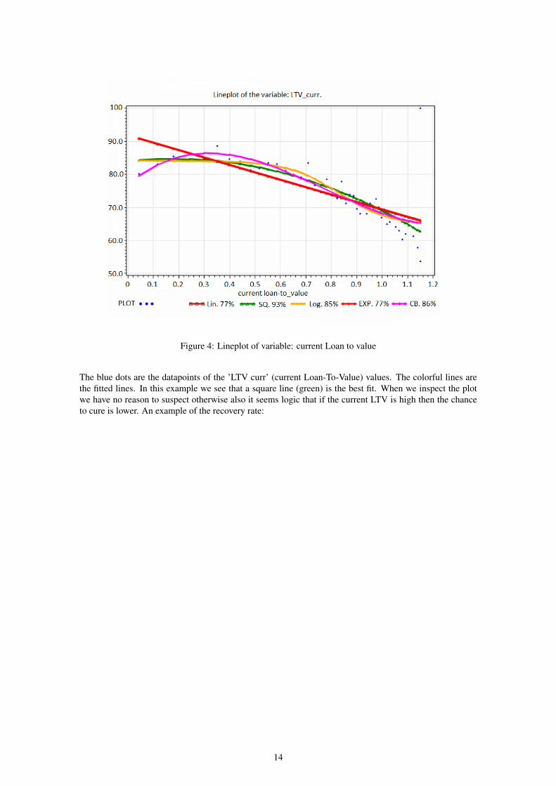
Figure 4: Lineplot of variable: current Loan to value

The blue dots are the datapoints of the ’LTV curr’ (current Loan-To-Value) values. The colorful lines arethe fitted lines. In this example we see that a square line (green) is the best fit. When we inspect the plotwe have no reason to suspect otherwise also it seems logic that if the current LTV is high then the chanceto cure is lower. An example of the recovery rate:

14

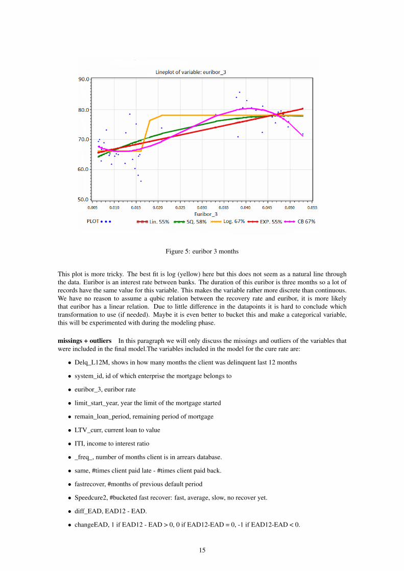
Figure 5: euribor 3 months

This plot is more tricky. The best fit is log (yellow) here but this does not seem as a natural line throughthe data. Euribor is an interest rate between banks. The duration of this euribor is three months so a lot ofrecords have the same value for this variable. This makes the variable rather more discrete than continuous.We have no reason to assume a qubic relation between the recovery rate and euribor, it is more likelythat euribor has a linear relation. Due to little difference in the datapoints it is hard to conclude whichtransformation to use (if needed). Maybe it is even better to bucket this and make a categorical variable,this will be experimented with during the modeling phase.

missings + outliers In this paragraph we will only discuss the missings and outliers of the variables thatwere included in the final model.The variables included in the model for the cure rate are:

• Delq_L12M, shows in how many months the client was delinquent last 12 months

• system_id, id of which enterprise the mortgage belongs to

• euribor_3, euribor rate

• limit_start_year, year the limit of the mortgage started

• remain_loan_period, remaining period of mortgage

• LTV_curr, current loan to value

• ITI, income to interest ratio

• _freq_, number of months client is in arrears database.

• same, #times client paid late - #times client paid back.

• fastrecover, #months of previous default period

• Speedcure2, #bucketed fast recover: fast, average, slow, no recover yet.

• diff_EAD, EAD12 - EAD.

• changeEAD, 1 if EAD12 - EAD > 0, 0 if EAD12-EAD = 0, -1 if EAD12-EAD < 0.

15

• LTV_risky1, Flag if LTV_curr > 1.

• arrearsflag, Flag if last record of client is an arrear in arrear database.

Missings + outliersVariable type missings outliersDelq_L12M basic 0 0system_id basic 0 0euribor_3 basic 0 0limit_start_year basic 0 0remain_loan_period basic 0 0LTV_curr basic 1757 3ITI basic 2811 60_freq_ created 0 0same created 0 0fastrecover created 0 0Speedcure2 created 0 0changeEAD created 5515 0diff_EAD created 5515 0LTV_risky1 created 0 0arrearsflag created 0 0

The final dataset we are using contains 67,300 records. We do not want to delete records because ofone of the risk drivers is missing so we will fill the missing values of ITI and LTV_curr with their mean.changeEAD and diff_EAD are created and contains missings because EAD and EAD 12 contains missings(the basic variables which they were created of). We will replace the missings of EAD and EAD12 withtheir means. By replacing these values we also remove the missing values in changeEAd and diff_EAD.

For the outliers we need to look more closer at the records. If we look at all records of ITI bigger than2 we have 95 records. We can immediately see the outliers since there is a big difference between thesevalues. The biggest reasonable record is 7.66. After 7.66 we only see values in 7000, 8000 or 9000. We de-cide that values above 7.66 are outliers and are deleted from the dataset. This results in 60 records deleted.For LTV_curr we only see three strange values in the dataset and all three are 9999.99. We decided to alsodelete these records from the dataset.

The records we are using for the cure rate and recovery rate are different. For the recovery rate we only use12387 records, the datasets are already pre-made and can contain different clients. Therefore we will needto analyze the variables again even though a couple might already have been analyzed for the cure rate. Forthe recovery rate we use the following variables:

• Delq_L12M, shows in how many months the client was delinquent last 12 months

• system_id, id of which enterprise the mortgage belongs to

• euribor_3, euribor rate

• limit_start_year, year the limit of the mortgage started

• remain_loan_period, remaining period of mortgage

• LTV_curr, current loan to value

• ITI, income to interest ratio

• NHG, flag if the customer has collateral on his mortgage.

• same, #times client paid late - #times client paid back.

• fastrecover, #months of previous default period

• Speedcure2, #bucketed fast recover: fast, average, slow, no recover yet.

• arrearsflag, Flag if last record of client is an arrear in arrear database.

16

• month_limit, Flag if last record of client is an arrear in arrear database.

• prv_kort, Flag if last record of client is an arrear in arrear database.

• diff_EAD, EAD12 - EAD.

• current_instalment, Flag if last record of client is an arrear in arrear database.

• EAD, Exposure at default of client

• AGE_curr, current age of client.

Missings + outliersVariable type missings outliersDelq_L12M basic 0 0system_id basic 0 0euribor_3 basic 0 0limit_start_year basic 0 0remain_loan_period basic 0 0LTV_curr basic 235 0ITI basic 437 10NHG basic 172 0same created 0 0fastrecover created 0 0Speedcure2 created 0 0month_limit created 0 0prv_kort created 0 0diff_EAD created 879 0current_instalment created 27 0arrearsflag created 0 0EAD created 27 0AGE_curr created 3 0

For LTV_curr, ITI, diff_EAD we apply the same methods as for the cure rate. Also we replace missingvalues of the variables, current_instalment, EAD, AGE_curr with their respective means. The only variablewith a different approach is NHG, which is a flag (boolean) and represents a 0 or 1. Since we only have12387 rows we do not want to delete any more records. We take a look at a bubble plot of NHG plottedagainst the recovery rate.

17

Figure 6: Bubble plot NHG

As we can see in the bubble plot mortgages without collateral (NHG = 0) recover on average less thanmortgages with collateral. This is a logical result. To be conservative we say that if NHG is missing we willput a 0 instead. Our model will then forecast a little bit more on the conservative side which is less risky. Ifwe look close at the plot we will see that the numbers do not add up to 12387, this is because we have runthe univariate analysis on a training set and not on the whole set.

additional node At the end of our research we ran the machine learning models which can handlemissing values (such as random forest) without replacing the missing values and without deletion. Aftercomparison with the ’cleaned’ dataset we saw that the models with the cleaned dataset performed better.

information value + c-stat information value (IV) and c-stat are both methods to assess the explanatorypower of a predictive variable regarding the target variable. For categorical variables we look at Informationvalue to classify predictive power. For continuous variables we look at the c-stat to determine the predictivepower of a variable. IV and c-stat both help us select good predictors for our final model.

IV =∑

(%non-events−%events) ∗WOE

In this case an event would be a cure and a non-event would be a non-cure. WOE stands for weight ofevidence which is derived by: ln(%non-events

%events ). For the recovery rate our target variable is continuous andwe cannot define properly an event and a non-event. The information value will only be calculated for thecure rate. For the recovery rate we will look at Spearman’s rank correlation and feature importance of thealgorithm plus the risk drivers of the cure rate models. The same holds for the c-statistic, it is a method toassess the predictive accuracy when the outcome is binary. We assess the variables by the following scoringrules:

IV Predictive power

< 0.1 weak predictor0.1 - 0.3 medium predictor

> 0.3 strong predictor

C-stat Predictive power

< 55% weak predictor55% - 60% medium predictor

> 60% strong predictor

18

For every variable either an IV or c-stat was derived, depending on the type of variable. The results for themodel variables of the cure rate are given below.

variable IV c-stat_FREQ_ - 0.76

same - 0.66fastRecover - 0.69SpeedCure2 0.58 -

DELQ_L12M - 0.59system_id 0 -euribor_3 - 0.58

limit_start_year - 0.57arrearsflag 0.22 -Diff_EAD - 0.54LTV_curr - 0.61

LTV_Risky1 0.14 -ITI - 0.52

changeEAD 0 -

As we can see changeEAD has no predicting power according to the IV. IV is very good in classifying binaryvariables but not that good in ordinal variables. changeEAD can be -1, 0 or 1, which are hard values for IVto do a good job, that is why the information value is low and we should not only look at the informationvalue or c-stat for variable selection. The Spearman rank scores for the recovery rate variables:

variable Spearman rankarrearsflag 0.27246

DELQ_L12M -0.10529Diff_EAD 0.12476

fastRecover -0.39146limit_start_year -0.09839

LTV_curr -0.32306NHG 0.14164same -0.32823

euribor_3 -0.08902MONTH_limit 0.18308

remain_loan_period -0.14226ITI -0.20902

current_instalment -0.17216EAD -0.20025

AGE_curr 0.09325

19

The higher the Spearman rank score the more informative the feature is. The feature with the highest rankscore is fastRecover (-0.39). The negative relation seems logical since it can be assumed that if the previousdefault was recovered fast that this default will have a higher recovery, due to reliable behavior. We observethat the features with the highest scores match the best features chosen by the algorithms.

transformations For logistic regression models we need variables on the same scale. Therefore a trans-formation (logistic, exponential, quadratic, linear or cubic) has been chosen for each variable as well, basedon the c-stat or information value, the fit of the function and business rationale. In some machine learn-ing models this is not necessary and we can use the original drivers. An example of the transformation-approach: The blue dots are the data points. We try to fit the best line through the points. the lines we use

Figure 7: lineplot of variable: current age

are, linear, square, logistic, exponential and cubic. For this plot, square and cubic are the best lines, whichlooks reasonable. We will summarize the results below, the plots can be found in the appendix. Only thecontinuous variables need to be transformed.

cure rate variables transformations

_FREQ_ logsame log

fastRecover logeuribor_3 cubic

limit_start_year cubicDiff_EAD logLTV_curr cubic

ITI cubic

recovery rate variables transformations

Delq_L12M logeuribor_3 log

limit_start_year cubicremain_loan_period cubic

LTV_curr logITI log

same logfastrecover log

month_limit cubicdiff_EAD log

current_instalment cubicEAD cubic

AGE_curr cubic

20

feature engineering After the calculation of IV and c-stat of the variables we tried to create own featureswhere the values of the IV and c-stat were high, to see if we could explain the data even better. Next tocreating extra features also the binning of several basic features was tried. A list of every created or binnedfeature:

1. leeftijdscategorie, binned age

2. Diff_months_OrderDate, difference between end of mortgage and order date of mortgage.

3. Diff_LDE, difference between end of mortgage and last default event.

4. Diff_NDM, length of performing period of mortgage.

5. Diff_Pod_Pid, lenght of previous default period.

6. sixmonthflag, Diff_months_OrderDate > 6 months

7. yearflag, Diff_months_OrderDate > 12 months

8. twoyearflag, Diff_months_OrderDate > 24 months

9. threeyearflag, Diff_months_OrderDate > 36 months

10. fouryearflag, Diff_months_OrderDate > 48 months

11. fiveyearflag, Diff_months_OrderDate > 60 months

12. Diff_EAD, EAD12 - EAD

13. Diff_OS, OS_init - OS

14. LTV_Risky1, LTV_curr > 1

15. CI_to_OS_ratio, = current installmentOS ∗ 100

16. AuctionCancel, flag if auction_date is filled.

17. ComparedDebtandRecovery = debt_on_auction_dateNHG_secrec

18. flag_LS, flag if loan_status_key = "LS"

19. flag_MR, flag if loan_status_key = "MR"

20. flagTopThree, flag if product type code is ’p1182’,’p1175’,’p1168’

21. debtpermonthOD, arrears / diff_months_orderdate

22. debtpermonthLDE, arrears/ diff_LDE

23. flagDODlow, flag if DebtPerMonthOD < 41.86;

24. arrearclass, binned arrears

25. diff_limit_year, difference between start of limit and today

26. workoutflag, flag if months_workout is filled

27. nextintodefflag, flag if next_int_def is filled

28. diffDefaultflag, flag if last default event 6= next_int_def

29. debtOnAUCflag, flag if there is debt on auction date.

30. changeEAD, 1 if diff_ead < 0, 0 if diff_ead = 0, -1 if diff_ead > 0

31. fastrecover, cure length of previous default period

32. sourceflags, binned source

33. flag65, flag if age_curr > 65

21

34. WWinst, mortg_market_value - EAD

35. regio, place of collateral

36. fleuribor, binned euribor

37. Delq_L12MBucket, binned delq_L12M

38. FEAD, binned EAD.

39. _freq_, months of client in arreardatabase

40. same, #times paid late - #times paid back

41. arrearsflag, flag if last record is an arrear.

Most of the features were for understanding the data but some explained the data really well and wereimplemented in the model. Some features were implemented but later removed because of correlation, badpredictive value or it gives information which may not be used. Some of these features can be improvedand many more can be introduced this will be discussed in the follow-up research section.

22

5 Methods and ModelsThis section will discuss the models that are used and their purpose.

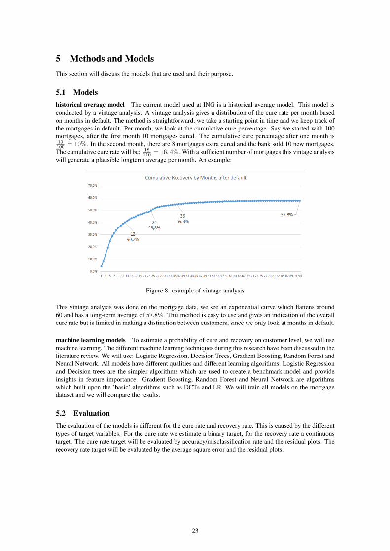
5.1 Modelshistorical average model The current model used at ING is a historical average model. This model isconducted by a vintage analysis. A vintage analysis gives a distribution of the cure rate per month basedon months in default. The method is straightforward, we take a starting point in time and we keep track ofthe mortgages in default. Per month, we look at the cumulative cure percentage. Say we started with 100mortgages, after the first month 10 mortgages cured. The cumulative cure percentage after one month is10100 = 10%. In the second month, there are 8 mortgages extra cured and the bank sold 10 new mortgages.The cumulative cure rate will be: 18

110 = 16, 4%. With a sufficient number of mortgages this vintage analysiswill generate a plausible longterm average per month. An example:

Figure 8: example of vintage analysis

This vintage analysis was done on the mortgage data, we see an exponential curve which flattens around60 and has a long-term average of 57.8%. This method is easy to use and gives an indication of the overallcure rate but is limited in making a distinction between customers, since we only look at months in default.

machine learning models To estimate a probability of cure and recovery on customer level, we will usemachine learning. The different machine learning techniques during this research have been discussed in theliterature review. We will use: Logistic Regression, Decision Trees, Gradient Boosting, Random Forest andNeural Network. All models have different qualities and different learning algorithms. Logistic Regressionand Decision trees are the simpler algorithms which are used to create a benchmark model and provideinsights in feature importance. Gradient Boosting, Random Forest and Neural Network are algorithmswhich built upon the ’basic’ algorithms such as DCTs and LR. We will train all models on the mortgagedataset and we will compare the results.

5.2 EvaluationThe evaluation of the models is different for the cure rate and recovery rate. This is caused by the differenttypes of target variables. For the cure rate we estimate a binary target, for the recovery rate a continuoustarget. The cure rate target will be evaluated by accuracy/misclassification rate and the residual plots. Therecovery rate target will be evaluated by the average square error and the residual plots.

23

6 Experimental SetupTo model the LGD we need to model the cure rate and recovery rate first. Both models will be trained andtested separately. We will have different sizes of datasets for both components as well. The cure rate willbe evaluated on misclassification rate and the recovery rate on the coefficient of determination. We willestimate the LGD for three different cases. LGD through the cycle (through the cycle), LGD in default andLGD in downturn. For each LGD-model we will specify the test & training set, the features, the algorithmsand the hyperparameters.

6.1 Training and TestingThe different sizes between the datasets are caused by different clients. Clients which do not cure will bein the recovery rate dataset. So our recovery rate dataset will always be smaller than our cure rate datasetfor every case. For LGD through the cycle we use all data provided by ING on client level. For LGD indownturn we take the same database but only of 1 year. So the dataset for downturn will be much smaller.For LGD in default we will transform the database from client level to month level, this means that we willhave a full overview per client. This results in an unfolded dataset which is much bigger than the orginaldatabase. The different databases summarized:

Dataset #rowsCure rate through the cycle 67300

Cure rate in default 129744Cure rate in downturn 7292

Recovery rate through the cycle 12478Recovery rate in default 60300

Recovery rate in downturn 2000

We part the datasets into an 80% training set and 20% test set. The training set is large enough to trainthe algorithm sufficiently, a 20% test set is also large enough for testing. For LGD in downturn we haverelatively few observations so we tested whether it is good to alter the training/test ratio.

Ratio 60/40 70/30 80/20 90/10cure rate (misclassification rate) 0.047 0.047 0.045 0.047

recovery rate (ASE) 0.051 0.052 0.045 0.049

This test is based on a random forest algorithm, we test on misclassification rate for cure rate and aver-age square error for recovery rate. We see that for the cure rate LGD in downturn the difference betweenthe ratios is very small. We observe that 90/10 leads to a worse result than 80/20 due to overtraining. ForLGD in downturn we will stay with the ratio 80/20. For the recovery rate we see bigger differences butalso that the 80/20 ratio gives the best performance. A notable observation is that the model performs betterunder a 60/40 rate than a 70/30 rate. This can happen especially when we have little data.

6.2 ExperimentsFor each case we will run five machine learning algorithms. LR, DCT, RF, GB and NN, we compareevery algorithm with each other based on important measurements. For the cure rate the measurements willbe: misclassification rate/accuracy, residual plot. For the recovery rate it will be: average square error,residual plot.

6.3 Hyperparameters optimizationThe more complex algorithms: Random Forest, Gradient Boosting and Neural net all have hyperparameters.These hyperparameters can be tuned for better results. For random forest and Gradient boosting we willuse Grid Search to optimize the hyperparameters.

Random forest The hyperparameters which will be optimized for random forest are:

• Leaf size

• Maximum debt

24

• Number of variables to consider

The leaf size specifies how many observations there should be in the last leaf. This is to catch noise andnot to overtrain the data with too many details. The maximum debt specifies how deep the trees can be,it reduces the complexity of trees and leads to lower chance of overfitting. The number of variables toconsider is to handle the variance/bias trade-off. If we consider all the variables at each split random forestwe continue to build the same tree over and over again which leads to low variance. If we consider onlya small number of variables each split we could end up with a lot of bad trees and a biased model. Thehyperparameter: ’number of variables to consider’ is to find balance between these two possibilities.

Gradient Boosting For gradient boosting the hyperparameters are:

• iterations

• shrinkage

• depth

• samples

Iterations stands for how many trees are built by the algorithm before quitting. In theory the more iterationsthe better the algorithm can predict but it can take up to a very long time to train all these trees. The iterationshyperparameter optimizes the tradeoff between processing time and learning growth of the algorithm to finda fast and precise model. Shrinkage is the concept of multiplying each step of the algorithm (building a treein this algorithm) by a factor between 0 and 1, called a learning rate. Shrinkage causes sample-predictionsto slowly converge toward observed values. Samples that get closer to their target end up being groupedtogether into larger and larger leaves, resulting in a natural regularization effect. The hyperparameter depthis the same as Maximum debt for random forest so to reduce complexity. The hyperparameter samples isto generate more different tree splits, which results in more information for the model. Gradient boostingalgorithms provide the ability to sample the data rows and columns before each boosting iteration, thisresults in more variance between the trees.

Neural Network For Neural Net we will run different auto neural nets which and see which performsbest. These auto neural nets are all differently shaped networks, we will try a block structure, a cascadestructure and a funnel structure. These networks provide a baseline model to see the type of network whichperforms best. The best performing network we will use for the competing neural network.

25

7 LGD in defaultFor LGD in default we will add "months in default" as a variable to the LGD through the cycle. The endgoal is to give a prediction of the probability of curing/recovering per month. To avoid bias in the modelwe need a specific sampling approach.

7.1 Sampling approachin default cure rate The modeling dataset is constructed by first extending the aforementioned startingdataset. Every default observation should be in the data as many times, as the months-workout. So for ex-ample, if a customer is 5 months in default, the number of rows for this particular customer should be 5 inthe in-default dataset. This approach is to enable inclusion of post-default information by inclusion of ref-erence moments. The risk driver information should be applicable at all the reference moments (e.g., LTVone month after default, two months after default, etc). Furthermore, the value of the months-in-defaultwill increase through the cycle in the data. The variables that remain the same through the cycle shouldbe copied throughout the history (like target variable that represents cure (cure flag) and the variable thatrepresents the random number (used to select the development dataset etc).

The constructed dataset cannot serve as a modeling dataset yet. This is because of the following reasons:

• Since the average workout period for cures and losses differ, the dataset will be not representative.

• Since one customer exists multiple times in the dataset, autocorrelation will occur leading to biasedestimations.

In order to deal with these issues, a stratified sampling approach should be applied (division into differentsubgroups or strata, then randomly select the final subjects proportionally from the different strata). Thesampling is based on months-in-default, and the following conditions with regard to the original cure ratetable and the sampled extended cure rate table apply:

1. distribution number of observations per months-in-default is equal

2. cure rate per months-in-default is equal

3. unique facilities is based on the same split of development vs. validation dataset (≈ 80%)

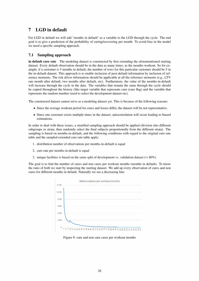
The goal is to find the number of cures and non cures per workout months (months in default). To knowthe ratio of both we start by inspecting the starting dataset. We add up every observation of cures and noncures for different months in default. Naturally we see a decreasing line:

Figure 9: cure and non cure cases per workout months

26

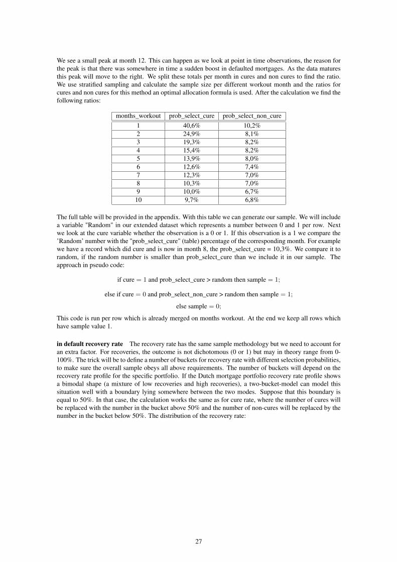
We see a small peak at month 12. This can happen as we look at point in time observations, the reason forthe peak is that there was somewhere in time a sudden boost in defaulted mortgages. As the data maturesthis peak will move to the right. We split these totals per month in cures and non cures to find the ratio.We use stratified sampling and calculate the sample size per different workout month and the ratios forcures and non cures for this method an optimal allocation formula is used. After the calculation we find thefollowing ratios:

months_workout prob_select_cure prob_select_non_cure1 40,6% 10,2%2 24,9% 8,1%3 19,3% 8,2%4 15,4% 8,2%5 13,9% 8,0%6 12,6% 7,4%7 12,3% 7,0%8 10,3% 7,0%9 10,0% 6,7%

10 9,7% 6,8%

The full table will be provided in the appendix. With this table we can generate our sample. We will includea variable "Random" in our extended dataset which represents a number between 0 and 1 per row. Nextwe look at the cure variable whether the observation is a 0 or 1. If this observation is a 1 we compare the’Random’ number with the "prob_select_cure" (table) percentage of the corresponding month. For examplewe have a record which did cure and is now in month 8, the prob_select_cure = 10,3%. We compare it torandom, if the random number is smaller than prob_select_cure than we include it in our sample. Theapproach in pseudo code:

if cure = 1 and prob_select_cure > random then sample = 1;

else if cure = 0 and prob_select_non_cure > random then sample = 1;

else sample = 0;

This code is run per row which is already merged on months workout. At the end we keep all rows whichhave sample value 1.

in default recovery rate The recovery rate has the same sample methodology but we need to account foran extra factor. For recoveries, the outcome is not dichotomous (0 or 1) but may in theory range from 0-100%. The trick will be to define a number of buckets for recovery rate with different selection probabilities,to make sure the overall sample obeys all above requirements. The number of buckets will depend on therecovery rate profile for the specific portfolio. If the Dutch mortgage portfolio recovery rate profile showsa bimodal shape (a mixture of low recoveries and high recoveries), a two-bucket-model can model thissituation well with a boundary lying somewhere between the two modes. Suppose that this boundary isequal to 50%. In that case, the calculation works the same as for cure rate, where the number of cures willbe replaced with the number in the bucket above 50% and the number of non-cures will be replaced by thenumber in the bucket below 50%. The distribution of the recovery rate:

27

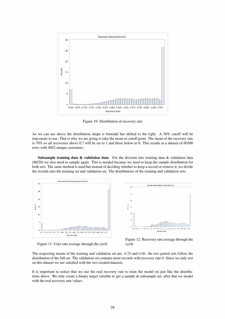
Figure 10: Distribution of recovery rate

As we can see above the distribution shape is bimodal but shifted to the right. A 50% cutoff will beinaccurate to use. That is why we are going to take the mean as cutoff point. The mean of the recovery rateis 70% so all recoveries above 0.7 will be set to 1 and those below to 0. This results in a dataset of 60300rows with 4042 unique customers.

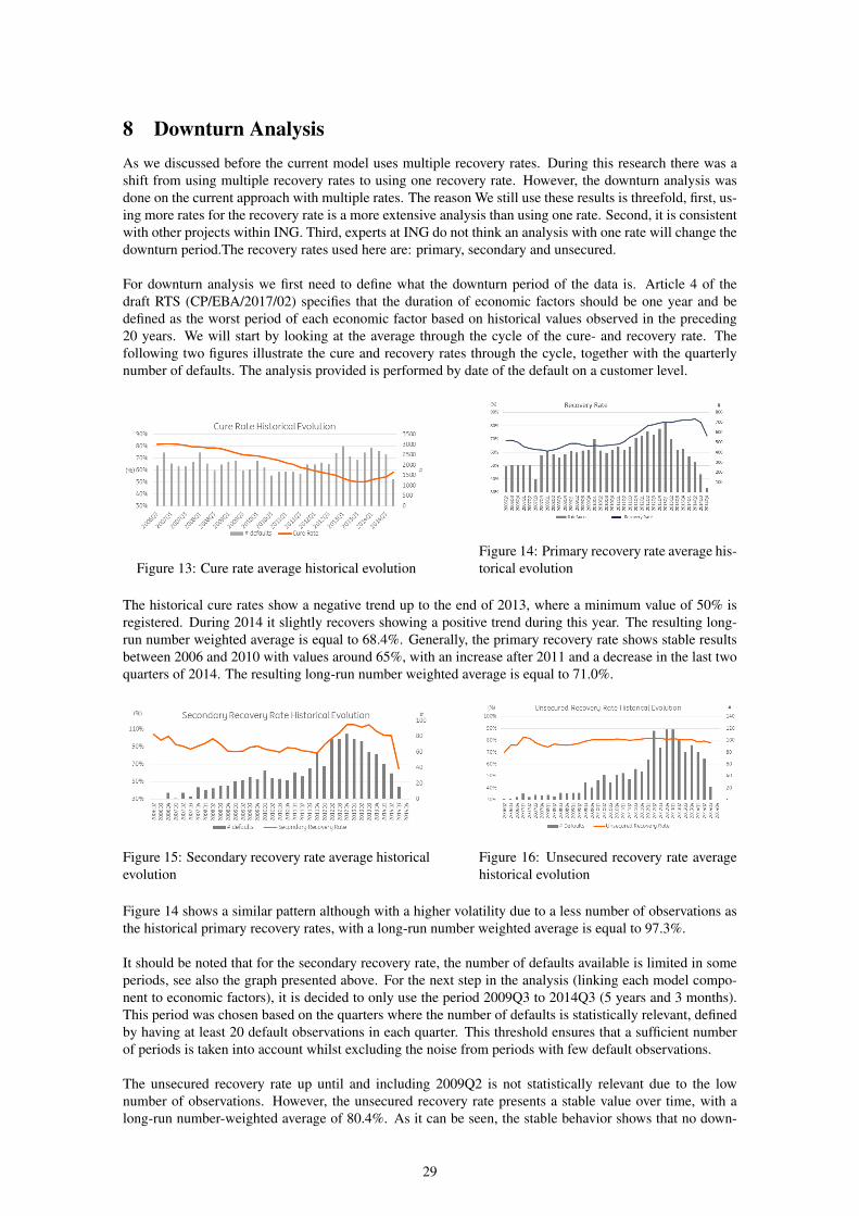
Subsample training data & validation data For the division into training data & validation data(80/20) we also need to sample again. This is needed because we need to keep the sample distribution forboth sets. The same method is used but instead of deciding whether to keep a record or remove it, we dividethe records into the training set and validation set. The distributions of the training and validation sets:

Figure 11: Cure rate average through the cycleFigure 12: Recovery rate average through thecycle

The respecting means of the training and validation set are: 0.70 and 0.66. the two parted sets follow thedistribution of the full set. The validation set contains more records with recovery rate 0. Since we only teston this dataset we are satisfied with the two created datasets.

It is important to notice that we use the real recovery rate to train the model on just like the distribu-tions above. We only create a binary target variable to get a sample & subsample set, after that we modelwith the real recovery rate values.

28

8 Downturn AnalysisAs we discussed before the current model uses multiple recovery rates. During this research there was ashift from using multiple recovery rates to using one recovery rate. However, the downturn analysis wasdone on the current approach with multiple rates. The reason We still use these results is threefold, first, us-ing more rates for the recovery rate is a more extensive analysis than using one rate. Second, it is consistentwith other projects within ING. Third, experts at ING do not think an analysis with one rate will change thedownturn period.The recovery rates used here are: primary, secondary and unsecured.

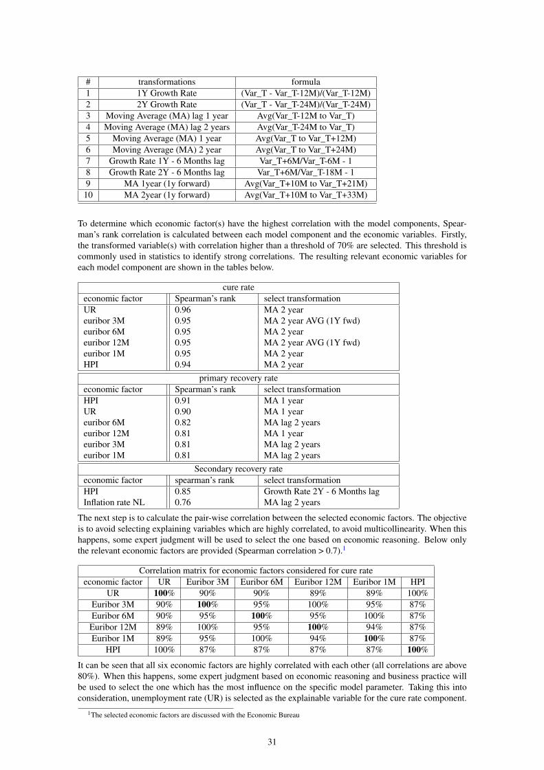
For downturn analysis we first need to define what the downturn period of the data is. Article 4 of thedraft RTS (CP/EBA/2017/02) specifies that the duration of economic factors should be one year and bedefined as the worst period of each economic factor based on historical values observed in the preceding20 years. We will start by looking at the average through the cycle of the cure- and recovery rate. Thefollowing two figures illustrate the cure and recovery rates through the cycle, together with the quarterlynumber of defaults. The analysis provided is performed by date of the default on a customer level.

Figure 13: Cure rate average historical evolutionFigure 14: Primary recovery rate average his-torical evolution

The historical cure rates show a negative trend up to the end of 2013, where a minimum value of 50% isregistered. During 2014 it slightly recovers showing a positive trend during this year. The resulting long-run number weighted average is equal to 68.4%. Generally, the primary recovery rate shows stable resultsbetween 2006 and 2010 with values around 65%, with an increase after 2011 and a decrease in the last twoquarters of 2014. The resulting long-run number weighted average is equal to 71.0%.

Figure 15: Secondary recovery rate average historicalevolution

Figure 16: Unsecured recovery rate averagehistorical evolution

Figure 14 shows a similar pattern although with a higher volatility due to a less number of observations asthe historical primary recovery rates, with a long-run number weighted average is equal to 97.3%.

It should be noted that for the secondary recovery rate, the number of defaults available is limited in someperiods, see also the graph presented above. For the next step in the analysis (linking each model compo-nent to economic factors), it is decided to only use the period 2009Q3 to 2014Q3 (5 years and 3 months).This period was chosen based on the quarters where the number of defaults is statistically relevant, definedby having at least 20 default observations in each quarter. This threshold ensures that a sufficient numberof periods is taken into account whilst excluding the noise from periods with few default observations.

The unsecured recovery rate up until and including 2009Q2 is not statistically relevant due to the lownumber of observations. However, the unsecured recovery rate presents a stable value over time, with along-run number-weighted average of 80.4%. As it can be seen, the stable behavior shows that no down-

29

turn effect exists for this component and therefore the described downturn approach is not applied for thiscomponent.

macro economic variables Next to the averages of all rates we will look at macro economic variables.To determine which economic factors are relevant for indicating the downturn period for each model com-ponent, a list of potential economic factors is considered, following Article 3(3) of the draft RTS (CP/E-BA/2017/02). The initial selected economic factors for this analysis are described in the table below:

# economic factor Description period source

1 GDP Absolute Growth DomesticProduct of NL

Jan 95 - Jun 17 Eurostat

2 UR Absolute UnemploymentRate in NL

Jan 95 - Aug 17 Eurostat

3 HPI Absolute House Price Index,with the index at 100 in 2010

Jan 95 - Aug 17 CBS

4 Euribor 1M Average interest rate atwhich Euro zone banksoffer unsecured loans onthe interbank market for amaturity of 1 months

Jan 95 - Apr 17 Bloomberg







8 inflation rate EU Inflation rate in the Eurozone, with the index at 100in 2015


9 Inflation rate NL Inflation rate in NL, with theindex at 100 in 2015


10 Dutch MortgateDefault rate

Internal average default rate Apr 06 - Oct 16 Internal

For statistical analysis of dependencies between economic factors and model components it is among othersrequired to take into account possible time lags between the realization of downturn in economic factors andthe possible impact on the model components. Typically the impact of a downturn is only visible in modelcomponents several months or years after the downturn is identified in the considered economic factor. Tofind the correlation between the economic factors and the model components it is easier to have a smoothcurve without any peaks in the data, also we are interested in the correlation of the trend between the com-ponent and the economic factor. For these reasons transformations and smoothing are used. Consequently,a number of transformations have been applied to each economic factor (see Table below), which meansa total of 100 economic variables transformations are analyzed for each model component. We will useMoving Average over 1 or 2 years.

30

# transformations formula1 1Y Growth Rate (Var_T - Var_T-12M)/(Var_T-12M)2 2Y Growth Rate (Var_T - Var_T-24M)/(Var_T-24M)3 Moving Average (MA) lag 1 year Avg(Var_T-12M to Var_T)4 Moving Average (MA) lag 2 years Avg(Var_T-24M to Var_T)5 Moving Average (MA) 1 year Avg(Var_T to Var_T+12M)6 Moving Average (MA) 2 year Avg(Var_T to Var_T+24M)7 Growth Rate 1Y - 6 Months lag Var_T+6M/Var_T-6M - 18 Growth Rate 2Y - 6 Months lag Var_T+6M/Var_T-18M - 19 MA 1year (1y forward) Avg(Var_T+10M to Var_T+21M)

10 MA 2year (1y forward) Avg(Var_T+10M to Var_T+33M)

To determine which economic factor(s) have the highest correlation with the model components, Spear-man’s rank correlation is calculated between each model component and the economic variables. Firstly,the transformed variable(s) with correlation higher than a threshold of 70% are selected. This threshold iscommonly used in statistics to identify strong correlations. The resulting relevant economic variables foreach model component are shown in the tables below.

cure rateeconomic factor Spearman’s rank select transformationUR 0.96 MA 2 yeareuribor 3M 0.95 MA 2 year AVG (1Y fwd)euribor 6M 0.95 MA 2 yeareuribor 12M 0.95 MA 2 year AVG (1Y fwd)euribor 1M 0.95 MA 2 yearHPI 0.94 MA 2 year

primary recovery rateeconomic factor Spearman’s rank select transformationHPI 0.91 MA 1 yearUR 0.90 MA 1 yeareuribor 6M 0.82 MA lag 2 yearseuribor 12M 0.81 MA 1 yeareuribor 3M 0.81 MA lag 2 yearseuribor 1M 0.81 MA lag 2 years

Secondary recovery rateeconomic factor spearman’s rank select transformationHPI 0.85 Growth Rate 2Y - 6 Months lagInflation rate NL 0.76 MA lag 2 years

The next step is to calculate the pair-wise correlation between the selected economic factors. The objectiveis to avoid selecting explaining variables which are highly correlated, to avoid multicollinearity. When thishappens, some expert judgment will be used to select the one based on economic reasoning. Below onlythe relevant economic factors are provided (Spearman correlation > 0.7).1

Correlation matrix for economic factors considered for cure rateeconomic factor UR Euribor 3M Euribor 6M Euribor 12M Euribor 1M HPI

UR 100% 90% 90% 89% 89% 100%Euribor 3M 90% 100% 95% 100% 95% 87%Euribor 6M 90% 95% 100% 95% 100% 87%Euribor 12M 89% 100% 95% 100% 94% 87%Euribor 1M 89% 95% 100% 94% 100% 87%

HPI 100% 87% 87% 87% 87% 100%

It can be seen that all six economic factors are highly correlated with each other (all correlations are above80%). When this happens, some expert judgment based on economic reasoning and business practice willbe used to select the one which has the most influence on the specific model parameter. Taking this intoconsideration, unemployment rate (UR) is selected as the explainable variable for the cure rate component.

1The selected economic factors are discussed with the Economic Bureau

31

Besides being an important economic factor where a decrease in unemployment makes it more likely thatclients will cure as it is more likely they will find a job and being able to pay their amount in arrears, thisvariable is also used earlier by ING in other models. This way, ING maintains consistency between differ-ent risk frameworks.

Correlation matrix for economic factors considered for primary recovery rateeconomic factor UR Euribor 3M Euribor 6M Euribor 12M Euribor 1M HPI

UR 100% 98% 91% 87% 91% 91%Euribor 3M 98% 100% 88% 91% 88% 89%Euribor 6M 91% 88% 100% 75% 100% 100%Euribor 12M 87% 91% 75% 100% 75% 76%Euribor 1M 91% 88% 100% 75% 100% 100%

HPI 91% 89% 100% 76% 100% 100%

The same six economic factors were selected as in the cure rate analysis and as such the same conclu-sion can be taken with all of them being highly correlated with each other. Again some expert judgmentbased on economic reasoning and business practice will be used to select the one which has the most in-fluence on the specific model parameter. Therefore for the Primary Recovery Rate, the selected economicfactor was the House Price Index as it directly impacts the recovery rate. As real estate prices move upor down, the value of the mortgage should also move in the same direction and therefore impacting therecovery amount.

Correlation matrix for economic factors considered for secondary recovery rateHPI inflation rate NL

HPI 100% 44%Inflation rate NL 3M 44% 100

For the secondary recovery rate, the two selected economic factors do not present a strong correlationbetween themselves. As both have a strong link with the secondary recovery rate, they were selected asrelevant economic factors. The final overview of the selected economic factors for the model componentfactors is present in the table below:

Component Economic factorsCure rate UR

Primary recovery rate HPISecondary recovery rate HPI & inflation rate NL

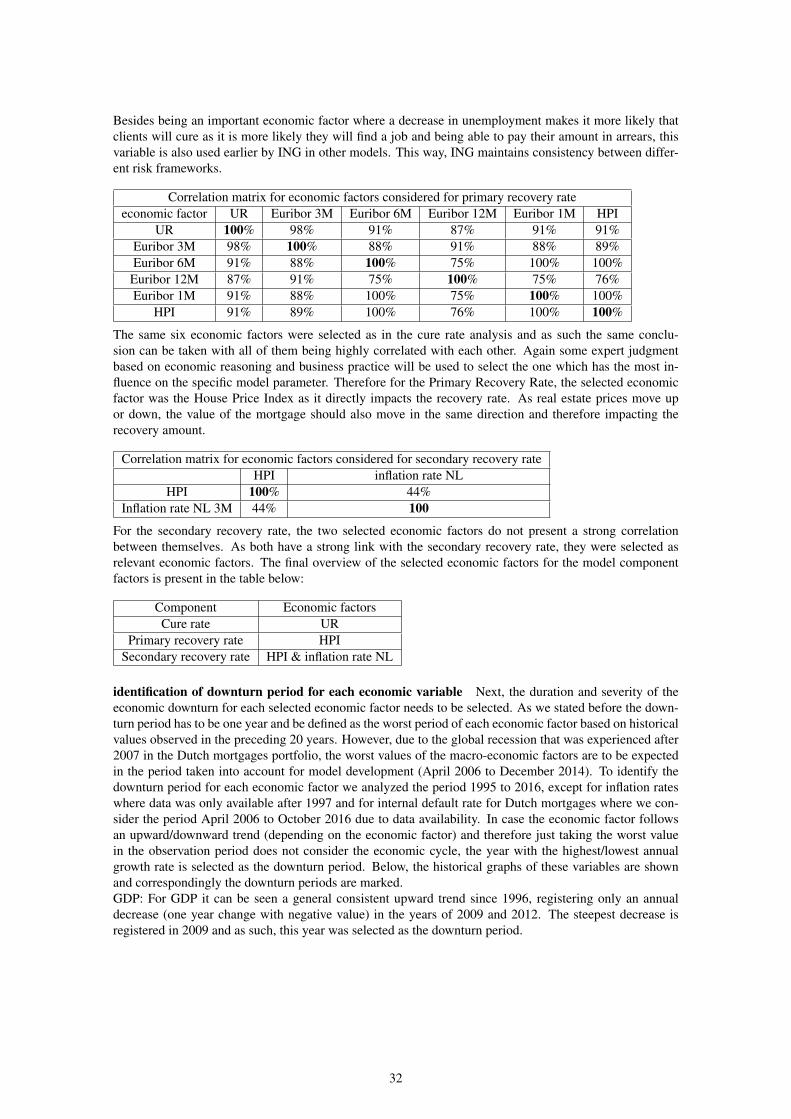
identification of downturn period for each economic variable Next, the duration and severity of theeconomic downturn for each selected economic factor needs to be selected. As we stated before the down-turn period has to be one year and be defined as the worst period of each economic factor based on historicalvalues observed in the preceding 20 years. However, due to the global recession that was experienced after2007 in the Dutch mortgages portfolio, the worst values of the macro-economic factors are to be expectedin the period taken into account for model development (April 2006 to December 2014). To identify thedownturn period for each economic factor we analyzed the period 1995 to 2016, except for inflation rateswhere data was only available after 1997 and for internal default rate for Dutch mortgages where we con-sider the period April 2006 to October 2016 due to data availability. In case the economic factor followsan upward/downward trend (depending on the economic factor) and therefore just taking the worst valuein the observation period does not consider the economic cycle, the year with the highest/lowest annualgrowth rate is selected as the downturn period. Below, the historical graphs of these variables are shownand correspondingly the downturn periods are marked.GDP: For GDP it can be seen a general consistent upward trend since 1996, registering only an annualdecrease (one year change with negative value) in the years of 2009 and 2012. The steepest decrease isregistered in 2009 and as such, this year was selected as the downturn period.

32

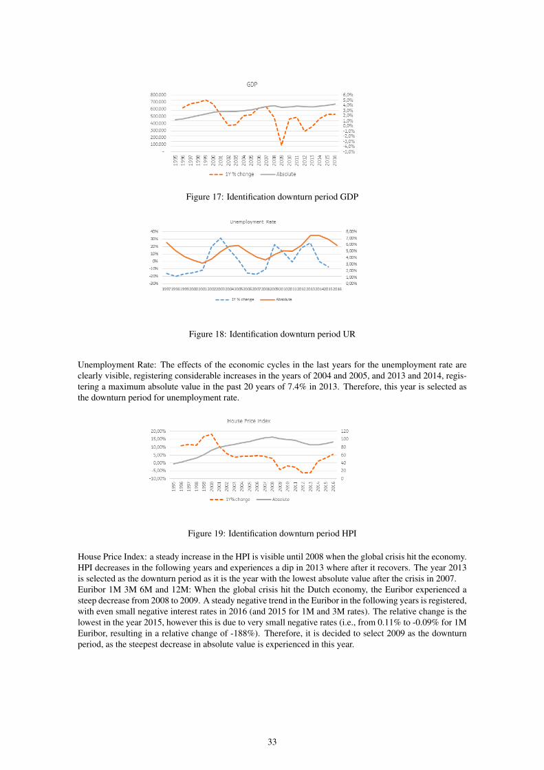
Figure 17: Identification downturn period GDP

Figure 18: Identification downturn period UR

Unemployment Rate: The effects of the economic cycles in the last years for the unemployment rate areclearly visible, registering considerable increases in the years of 2004 and 2005, and 2013 and 2014, regis-tering a maximum absolute value in the past 20 years of 7.4% in 2013. Therefore, this year is selected asthe downturn period for unemployment rate.

Figure 19: Identification downturn period HPI

House Price Index: a steady increase in the HPI is visible until 2008 when the global crisis hit the economy.HPI decreases in the following years and experiences a dip in 2013 where after it recovers. The year 2013is selected as the downturn period as it is the year with the lowest absolute value after the crisis in 2007.Euribor 1M 3M 6M and 12M: When the global crisis hit the Dutch economy, the Euribor experienced asteep decrease from 2008 to 2009. A steady negative trend in the Euribor in the following years is registered,with even small negative interest rates in 2016 (and 2015 for 1M and 3M rates). The relative change is thelowest in the year 2015, however this is due to very small negative rates (i.e., from 0.11% to -0.09% for 1MEuribor, resulting in a relative change of -188%). Therefore, it is decided to select 2009 as the downturnperiod, as the steepest decrease in absolute value is experienced in this year.

33

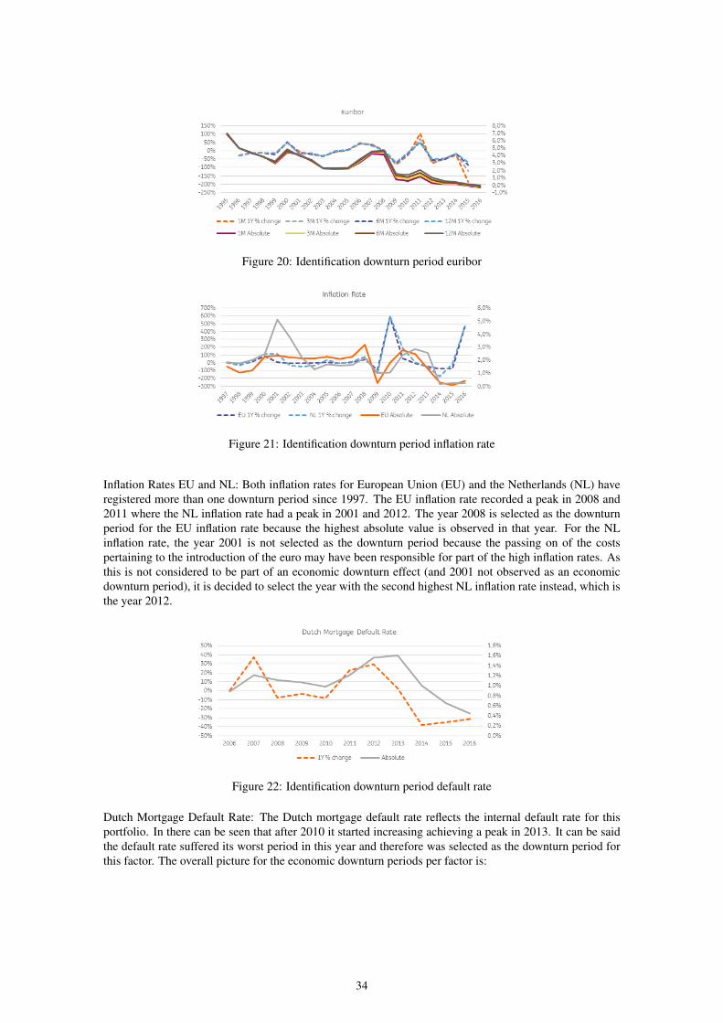
Figure 20: Identification downturn period euribor

Figure 21: Identification downturn period inflation rate

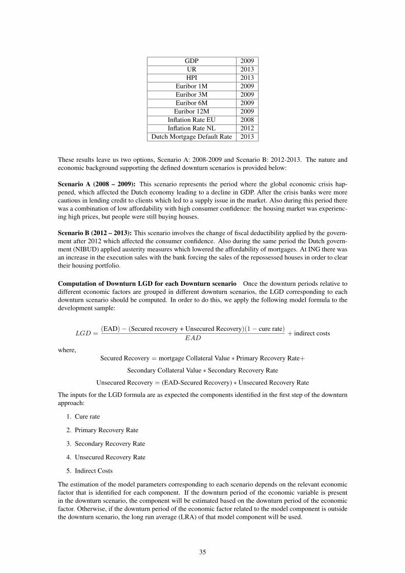
Inflation Rates EU and NL: Both inflation rates for European Union (EU) and the Netherlands (NL) haveregistered more than one downturn period since 1997. The EU inflation rate recorded a peak in 2008 and2011 where the NL inflation rate had a peak in 2001 and 2012. The year 2008 is selected as the downturnperiod for the EU inflation rate because the highest absolute value is observed in that year. For the NLinflation rate, the year 2001 is not selected as the downturn period because the passing on of the costspertaining to the introduction of the euro may have been responsible for part of the high inflation rates. Asthis is not considered to be part of an economic downturn effect (and 2001 not observed as an economicdownturn period), it is decided to select the year with the second highest NL inflation rate instead, which isthe year 2012.

Figure 22: Identification downturn period default rate

Dutch Mortgage Default Rate: The Dutch mortgage default rate reflects the internal default rate for thisportfolio. In there can be seen that after 2010 it started increasing achieving a peak in 2013. It can be saidthe default rate suffered its worst period in this year and therefore was selected as the downturn period forthis factor. The overall picture for the economic downturn periods per factor is:

34

GDP 2009UR 2013HPI 2013

Euribor 1M 2009Euribor 3M 2009Euribor 6M 2009Euribor 12M 2009

Inflation Rate EU 2008Inflation Rate NL 2012

Dutch Mortgage Default Rate 2013

These results leave us two options, Scenario A: 2008-2009 and Scenario B: 2012-2013. The nature andeconomic background supporting the defined downturn scenarios is provided below:

Scenario A (2008 – 2009): This scenario represents the period where the global economic crisis hap-pened, which affected the Dutch economy leading to a decline in GDP. After the crisis banks were morecautious in lending credit to clients which led to a supply issue in the market. Also during this period therewas a combination of low affordability with high consumer confidence: the housing market was experienc-ing high prices, but people were still buying houses.

Scenario B (2012 – 2013): This scenario involves the change of fiscal deductibility applied by the govern-ment after 2012 which affected the consumer confidence. Also during the same period the Dutch govern-ment (NIBUD) applied austerity measures which lowered the affordability of mortgages. At ING there wasan increase in the execution sales with the bank forcing the sales of the repossessed houses in order to cleartheir housing portfolio.

Computation of Downturn LGD for each Downturn scenario Once the downturn periods relative todifferent economic factors are grouped in different downturn scenarios, the LGD corresponding to eachdownturn scenario should be computed. In order to do this, we apply the following model formula to thedevelopment sample:

LGD =(EAD)− (Secured recovery + Unsecured Recovery)(1− cure rate)

EAD+ indirect costs

where,Secured Recovery = mortgage Collateral Value ∗ Primary Recovery Rate+

Secondary Collateral Value ∗ Secondary Recovery Rate

Unsecured Recovery = (EAD-Secured Recovery) ∗ Unsecured Recovery Rate

The inputs for the LGD formula are as expected the components identified in the first step of the downturnapproach:

1. Cure rate

2. Primary Recovery Rate

3. Secondary Recovery Rate

4. Unsecured Recovery Rate

5. Indirect Costs

The estimation of the model parameters corresponding to each scenario depends on the relevant economicfactor that is identified for each component. If the downturn period of the economic variable is presentin the downturn scenario, the component will be estimated based on the downturn period of the economicfactor. Otherwise, if the downturn period of the economic factor related to the model component is outsidethe downturn scenario, the long run average (LRA) of that model component will be used.

35

Year Cure Rate Primary Rec Rate Secondary Rec Rate Unsecured Rec RateLRA 68.4% 71.0% 97.3% 80.4%2006 81.9% 69.9% 105.9% 60.8%2007 82.1% 64.3% 92.5% 82.3%2008 79.6% 60.9% 94.3% 74.5%2009 76.5% 66.7% 84.7% 76.7%2010 72.1% 65.2% 87.6% 80.4%2011 66.5% 66.2% 88.6% 80.6%2012 59.8% 76.7% 92.3% 81.7%2013 53.3% 82.7% 115.3% 81.4%2014 52.0% 84.2% 103.4% 78.5%

Consider the Cure Rate where the relevant economic factor for this component is the unemployment rate.Therefore the downturn period is the year 2013 which is present in the downturn scenario B. So for thescenario A, the LRA will be used to calculate the overall LGD where in scenario B the average cure ratevalue for 2013 will be used, i.e. 53.3%. When more than one economic factor is identified for a componentfactor, the worst value of the selected years is chosen.

Model component Scenario A Scenario BCure Rate LRA 2013

Primary recovery Rate LRA 2012Secondary recovery Rate LRA 2012Unsecured recovery Rate LRA LRA

Indirect costs LRA LRA

This leads to the following downturn model component estimations and corresponding downturn LGDs:

Scenario A Value PeriodCure rate 68.4% LRA

Primary recovery Rate 71.0% LRASecondary recovery Rate 97.3% LRAUnsecured recovery Rate 80.4% LRA

Indirect costs 0.32 LRALGD 9.47

Scenario B Value PeriodCure rate 53.3% 2013

Primary recovery Rate 76.7% 2012Secondary recovery Rate 92.3% 2012Unsecured recovery Rate 80.4% LRA

Indirect costs 0.32% LRALGD 10.96%

The downturn scenario associated with the highest LGD is chosen as the final downturn scenario. Below, itcan be seen how the LGD through the cycle behaves for scenarios A and B compared to the observed losscases (not including dragging cases):

Figure 23: LGD through the cycle

36

Consequently, based on the results in the previous section and looking at the graph presented, Scenario Bis chosen as the final downturn scenario. It can be seen that Scenario B always has a higher LGD valuethan Scenario A. Moreover, the LGD of scenario B is higher than the observed loss rate over the entireperiod while the current LGD model (LGD Model V4) has a much higher value than the LGD in both theScenarios A and B. This demonstrates that the current model approach is sufficiently conservative

MoC for downturn Related to the Margin of Conservatism (MoC) and the downturn approach, a com-prehensive analysis should be performed, calibrating the MoC around the assumptions made for the identi-fication of the nature of the economic downturn. The MoC should be namely applied:

• When the analysis of the nature of the economic downturn shows no dependency between the modelcomponents and the economic indicators;

• When it is not possible to identify the severity of the economic downturn for a specific economicfactor according to historical data;

• No data availability concerning the realized model components during the selected economic down-turn period which are therefore estimated it for downturn adjustment purposes.

37

9 ResultsIn this section the results of each case will be discussed for the cure rate and recovery rate. Afterward, theLGD will be visualized and compared with the current model. The final cure rate models will be discussedin the section Experiment cure rate & Experiment recovery rate. First, we will show the findings we hadwith the first models of the cure rate component.

gap analysis The first benchmark models for the cure rate were flawed, it predicted well but there was astrange gap in the prediction, to illustrate:

Figure 24: RF cure rate model 2014-2016

This illustration represents a random forest cure rate model. Per quarter from 2006-2017 the averages ofthe actual cure rate and the predicted cure rate are visualized The blue line is the actual average of thedataset, the orange line is the predicted average of the algorithm. The residual error is the overall differencebetween the actual cure and the predicted cure. As the graph above shows, the orange line follows theblue line very well except for the period 2014-2016. This model was calculated with a 70/30 ratio and thefollowing variables:

• DELQ_L12M

• EAD

• LTV_Risky1

• NHG

• SpeedCure2

• _FREQ_

• arrearclass

• limit_start_year

• arrearsflag

• changeEAD

• fastRecover

• same

A residual error of 2.5 is not high when we consider the number of observations, it means that per observa-tion on average we make an error of 7.13E-05. Per quarter it means an average mistake of 5%. These errorsare mainly caused by the wide gap, so we analyzed this. Experts in the LGD field of ING did not recollectany big event in the period 2014-2016 which might lead to trend breaking. So we tried narrow the gap byusing:

1. other algorithms

2. varying the training/test ratio

3. sampling

38

4. changing the input variables

For every variation on the random forest (or other) model we trained with the dataset and the same test set.Other algorithms gave the same trend as random forest. For the ratio and sampling changes we saw thefollowing results:

Figure 25: Ratio change 70/30 to 80/20 Figure 26: Stratified sampling applied on dataset

Both changes result in a small performance improvement in the 2014-2016 period. The residual error dropsa little when we adjust the ratio, this is in line with our findings in the experimental setup section. If weapply sampling on the dataset we see that the error in the period 2014-2016 drops but overall the errorincreases, also the graph looks unstable. Both approaches do not narrow the gap sufficiently. Next we trychanging the input variables of the algorithm. First we model the period 2014-2016 to see which variablesare good predictors for that period. The results:

Figure 27: RF cure rate model 2014-2016

39

The fitted line estimates the actual line very well. When we take a look at the important features for thismodel we see some differences:

Differences in top variables between first model and 2014-2016 model2014-2016 model variables First model variables

_FREQ_ DELQ_L12Msame EAD

fastRecover LTV_Risky1SpeedCure2 NHG

DELQ_L12M SpeedCure2system_id _FREQ_arrearsflag arrearclass

limit_start_year arrearsflageuribor_3 changeEADLTV_curr fastRecover

remain_loan_period limit_start_yearDiff_EAD same

EAD, LTV_Risky1, NHG, arrearclass and changeEAD are out of the top predicting variables. system_id,euribor_3, LTV_curr, remain_loan_period and Diff_EAD replaced them in predicting ranking list. Whenwe apply these variables to the full dataset we observe the current random forest model: The error has been

Figure 28: Cure rate model RF

cut from 2.5 to 1.25 and during the gap period the error decreased by almost 1. The gap analysis has shownus which variables predict better and which ratio to handle.

9.1 Experiment cure rateHere we will discuss the component cure rate, we will discuss the model parameters, the performance andthe important features. In the end we will compare and choose the best model.

hyperparameters We will evaluate the hyperparameters we discussed in the experimental setup. We alsodiscuss the difference between the hyperparameters in the three cases: LGD through the cycle, LGD indefault and LGD in downturn. We will only show tables of the results. The graphs are in the appendix.First we inspect the cure rate.

40

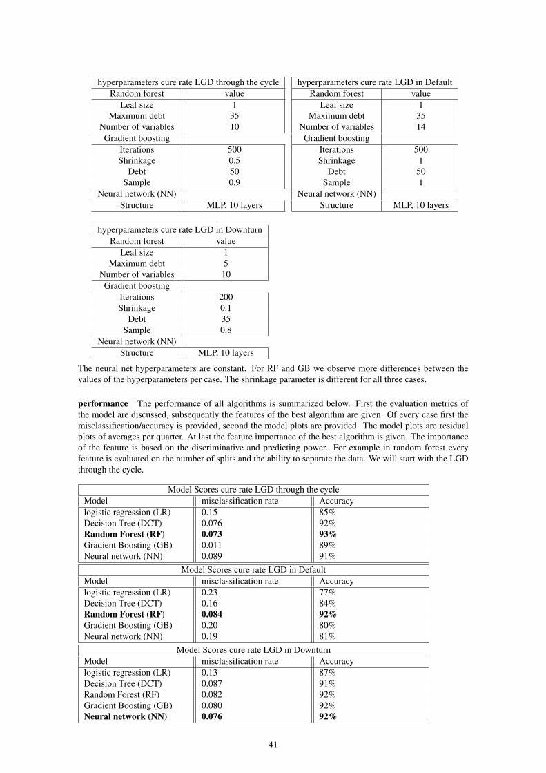
hyperparameters cure rate LGD through the cycleRandom forest value

Leaf size 1Maximum debt 35

Number of variables 10Gradient boosting

Iterations 500Shrinkage 0.5

Debt 50Sample 0.9

Neural network (NN)Structure MLP, 10 layers

hyperparameters cure rate LGD in DefaultRandom forest value



Iterations 500Shrinkage 1

Debt 50Sample 1


hyperparameters cure rate LGD in DownturnRandom forest value




Debt 35Sample 0.8


The neural net hyperparameters are constant. For RF and GB we observe more differences between thevalues of the hyperparameters per case. The shrinkage parameter is different for all three cases.

performance The performance of all algorithms is summarized below. First the evaluation metrics ofthe model are discussed, subsequently the features of the best algorithm are given. Of every case first themisclassification/accuracy is provided, second the model plots are provided. The model plots are residualplots of averages per quarter. At last the feature importance of the best algorithm is given. The importanceof the feature is based on the discriminative and predicting power. For example in random forest everyfeature is evaluated on the number of splits and the ability to separate the data. We will start with the LGDthrough the cycle.

Model Scores cure rate LGD through the cycleModel misclassification rate Accuracylogistic regression (LR) 0.15 85%Decision Tree (DCT) 0.076 92%Random Forest (RF) 0.073 93%Gradient Boosting (GB) 0.011 89%Neural network (NN) 0.089 91%

Model Scores cure rate LGD in DefaultModel misclassification rate Accuracylogistic regression (LR) 0.23 77%Decision Tree (DCT) 0.16 84%Random Forest (RF) 0.084 92%Gradient Boosting (GB) 0.20 80%Neural network (NN) 0.19 81%

Model Scores cure rate LGD in DownturnModel misclassification rate Accuracylogistic regression (LR) 0.13 87%Decision Tree (DCT) 0.087 91%Random Forest (RF) 0.082 92%Gradient Boosting (GB) 0.080 92%Neural network (NN) 0.076 92%

41

Above we see three tables of the model scores for each case. Each model is scored on their misclassifi-cation rate/accuracy. We see that Logistic Regression performs the worst each time. Random forest doesthe best job of classifying the customers. All scores are well above 80% and most even above 90%. Thisshows excellent models. We compare it with the residual plots of the model. In the next pages the modelplots will be discussed.

42

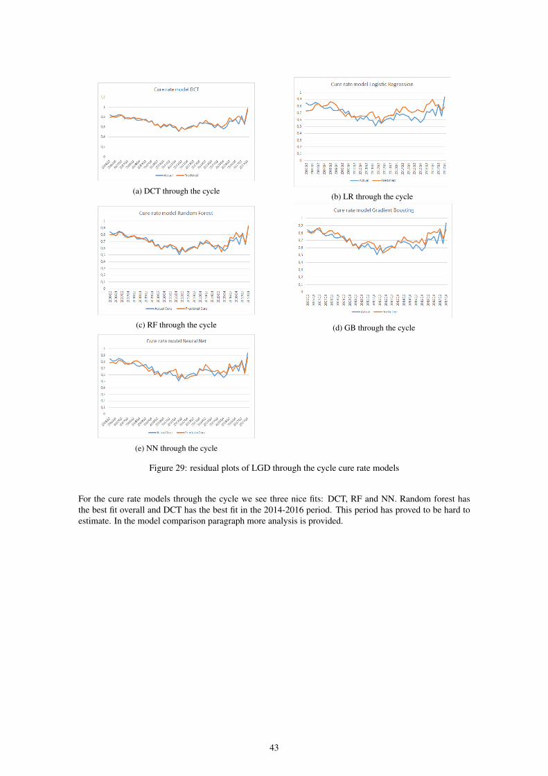
(a) DCT through the cycle(b) LR through the cycle

(c) RF through the cycle (d) GB through the cycle

(e) NN through the cycle

Figure 29: residual plots of LGD through the cycle cure rate models

For the cure rate models through the cycle we see three nice fits: DCT, RF and NN. Random forest hasthe best fit overall and DCT has the best fit in the 2014-2016 period. This period has proved to be hard toestimate. In the model comparison paragraph more analysis is provided.

43

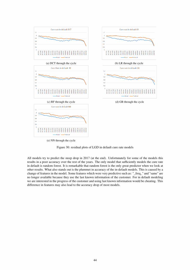
(a) DCT through the cycle (b) LR through the cycle



Figure 30: residual plots of LGD in default cure rate models

All models try to predict the steep drop in 2017 (at the end). Unfortunately for some of the models thisresults in a poor accuracy over the rest of the years. The only model that sufficiently models the cure ratein default is random forest. It is remarkable that random forest is the only great predictor when we look atother results. What also stands out is the plummet in accuracy of the in-default models. This is caused by achange of features in the model. Some features which were very predictive such as: "_freq_" and "same" areno longer available because they use the last known information of the customer. For in default modelingwe are interested in the progress of the customer and using last known information would be cheating. Thisdifference in features may also lead to the accuracy drop of most models.

44

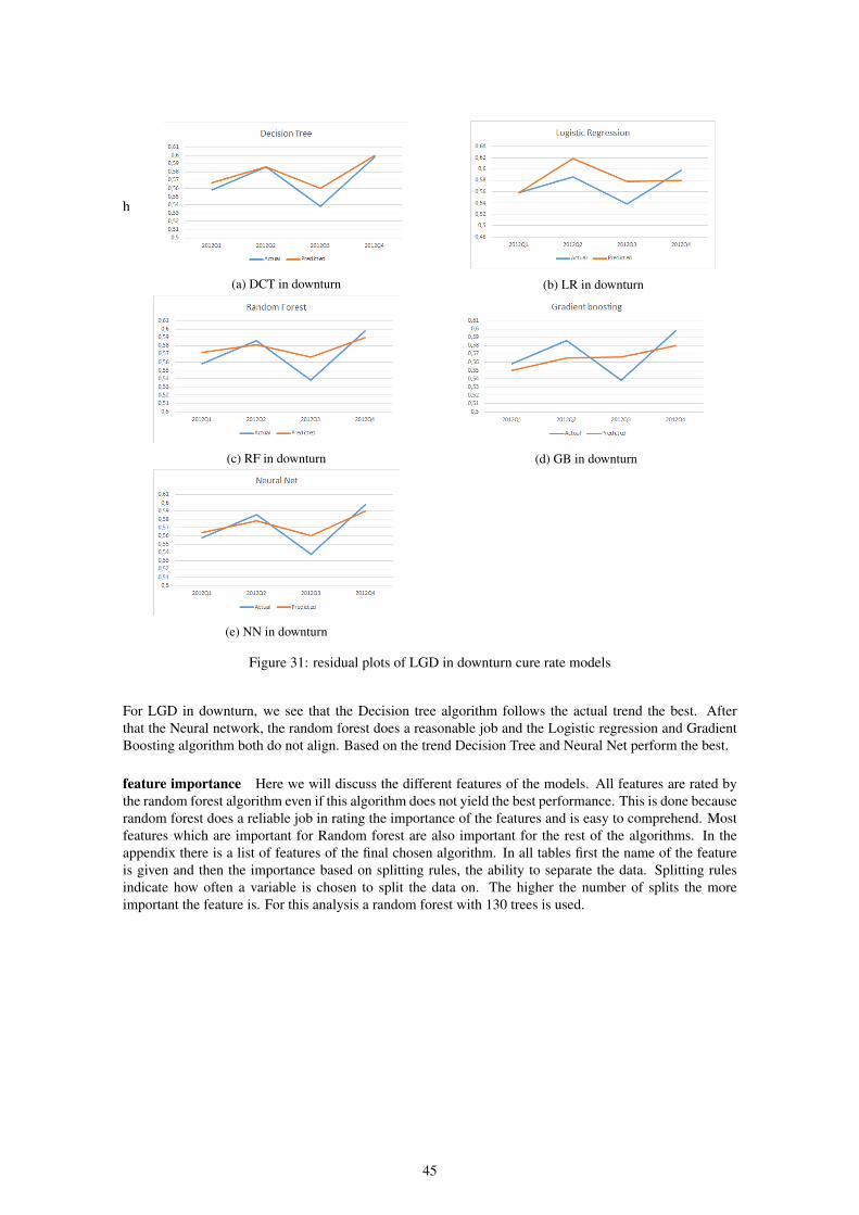
h

(a) DCT in downturn (b) LR in downturn

(c) RF in downturn (d) GB in downturn

(e) NN in downturn

Figure 31: residual plots of LGD in downturn cure rate models

For LGD in downturn, we see that the Decision tree algorithm follows the actual trend the best. Afterthat the Neural network, the random forest does a reasonable job and the Logistic regression and GradientBoosting algorithm both do not align. Based on the trend Decision Tree and Neural Net perform the best.

feature importance Here we will discuss the different features of the models. All features are rated bythe random forest algorithm even if this algorithm does not yield the best performance. This is done becauserandom forest does a reliable job in rating the importance of the features and is easy to comprehend. Mostfeatures which are important for Random forest are also important for the rest of the algorithms. In theappendix there is a list of features of the final chosen algorithm. In all tables first the name of the featureis given and then the importance based on splitting rules, the ability to separate the data. Splitting rulesindicate how often a variable is chosen to split the data on. The higher the number of splits the moreimportant the feature is. For this analysis a random forest with 130 trees is used.

45

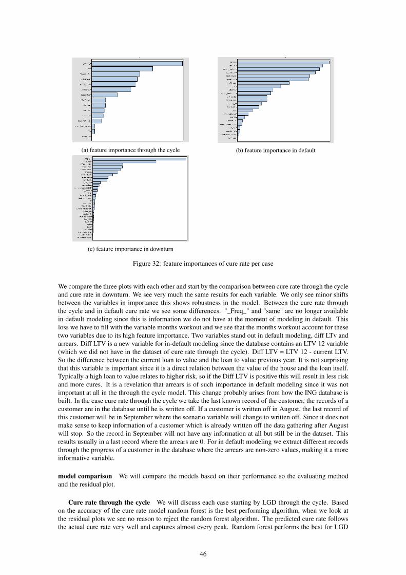
(a) feature importance through the cycle (b) feature importance in default

(c) feature importance in downturn

Figure 32: feature importances of cure rate per case

We compare the three plots with each other and start by the comparison between cure rate through the cycleand cure rate in downturn. We see very much the same results for each variable. We only see minor shiftsbetween the variables in importance this shows robustness in the model. Between the cure rate throughthe cycle and in default cure rate we see some differences. "_Freq_" and "same" are no longer availablein default modeling since this is information we do not have at the moment of modeling in default. Thisloss we have to fill with the variable months workout and we see that the months workout account for thesetwo variables due to its high feature importance. Two variables stand out in default modeling, diff LTv andarrears. Diff LTV is a new variable for in-default modeling since the database contains an LTV 12 variable(which we did not have in the dataset of cure rate through the cycle). Diff LTV = LTV 12 - current LTV.So the difference between the current loan to value and the loan to value previous year. It is not surprisingthat this variable is important since it is a direct relation between the value of the house and the loan itself.Typically a high loan to value relates to higher risk, so if the Diff LTV is positive this will result in less riskand more cures. It is a revelation that arrears is of such importance in default modeling since it was notimportant at all in the through the cycle model. This change probably arises from how the ING database isbuilt. In the case cure rate through the cycle we take the last known record of the customer, the records of acustomer are in the database until he is written off. If a customer is written off in August, the last record ofthis customer will be in September where the scenario variable will change to written off. Since it does notmake sense to keep information of a customer which is already written off the data gathering after Augustwill stop. So the record in September will not have any information at all but still be in the dataset. Thisresults usually in a last record where the arrears are 0. For in default modeling we extract different recordsthrough the progress of a customer in the database where the arrears are non-zero values, making it a moreinformative variable.

model comparison We will compare the models based on their performance so the evaluating methodand the residual plot.

Cure rate through the cycle We will discuss each case starting by LGD through the cycle. Basedon the accuracy of the cure rate model random forest is the best performing algorithm, when we look atthe residual plots we see no reason to reject the random forest algorithm. The predicted cure rate followsthe actual cure rate very well and captures almost every peak. Random forest performs the best for LGD

46

through the cycle.

Cure rate in default It is very clear that RF outperforms any other model for this case. Both theaccuracy and the residual plot show the best results. RF should be used to model in default cure rate.

Cure rate in downturn At last for LGD in downturn we observe that NN does the best job in termsof accuracy. The residual plots show two algorithms which capture the actual cure rate sufficiently, DCTand NN. DCT seems to do a slightly better job but NN is more conservative. Since the ECB maintains strictrules about a conservative approach we will give the edge to NN for LGD in downturn.

9.2 Experiment recovery rateFor the recovery rate the same approach as the cure rate is taken. First the hyperparameters, then theperformance and at the end the model comparison.

hyperparameters The algorithms for the recovery rate are the same, this means that the hyperparametersfor the recovery rate are also the same. Logically the values can differ, we observe:

hyperparameters RR LGD through the cycleRandom forest value




Debt 50Sample 0.9


hyperparameters recovery rate LGD in DefRandom forest value




Debt 35Sample 0.9


hyperparameters recovery rate LGD in DownturnRandom forest value




Debt 35Sample 0.8


performance To find the right model for the recovery rate we will evaluate the performance of the modelson Average square error (ASE), residual plots.

Model Scores recovery rate LGD through the cycleModel Average Square Error (ASE)linear regression (LR) 0.042Decision Tree (DCT) 0.040Random Forest (RF) 0.038Gradient Boosting (GB) 0.037Neural network (NN) 0.040

47

Model Scores recovery rate LGD in defaultModel Average Square Error (ASE)linear regression (LR) 0.057Decision Tree (DCT) 0.032Random Forest (RF) 0.014Gradient Boosting (GB) 0.044Neural network (NN) 0.047

Model Scores recovery rate LGD in downturnModel Average Square Error (ASE)linear regression (LR) 0.046Decision Tree (DCT) 0.048Random Forest (RF) 0.045Gradient Boosting (GB) 0.046Neural network (NN) 0.048

For each case the model scores have been given. We first compare the models based on their ASE. Gradientboosting does the best job in modeling the recovery rate through the cycle based on ASE. For the downturnperiod random forest performs better in terms of ASE. The differences are small so we need the residualplots to decide which is the best.

48

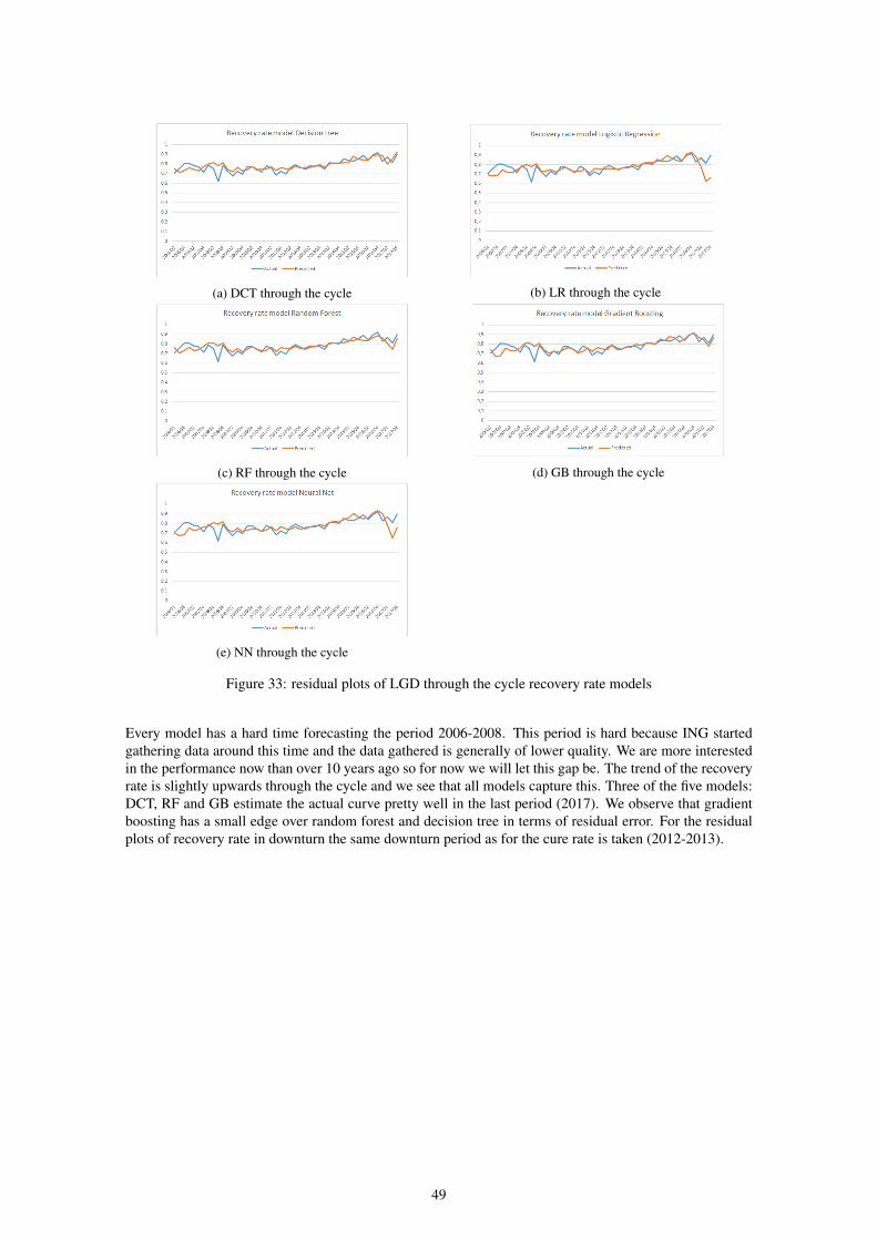
(a) DCT through the cycle (b) LR through the cycle



Figure 33: residual plots of LGD through the cycle recovery rate models

Every model has a hard time forecasting the period 2006-2008. This period is hard because ING startedgathering data around this time and the data gathered is generally of lower quality. We are more interestedin the performance now than over 10 years ago so for now we will let this gap be. The trend of the recoveryrate is slightly upwards through the cycle and we see that all models capture this. Three of the five models:DCT, RF and GB estimate the actual curve pretty well in the last period (2017). We observe that gradientboosting has a small edge over random forest and decision tree in terms of residual error. For the residualplots of recovery rate in downturn the same downturn period as for the cure rate is taken (2012-2013).

49

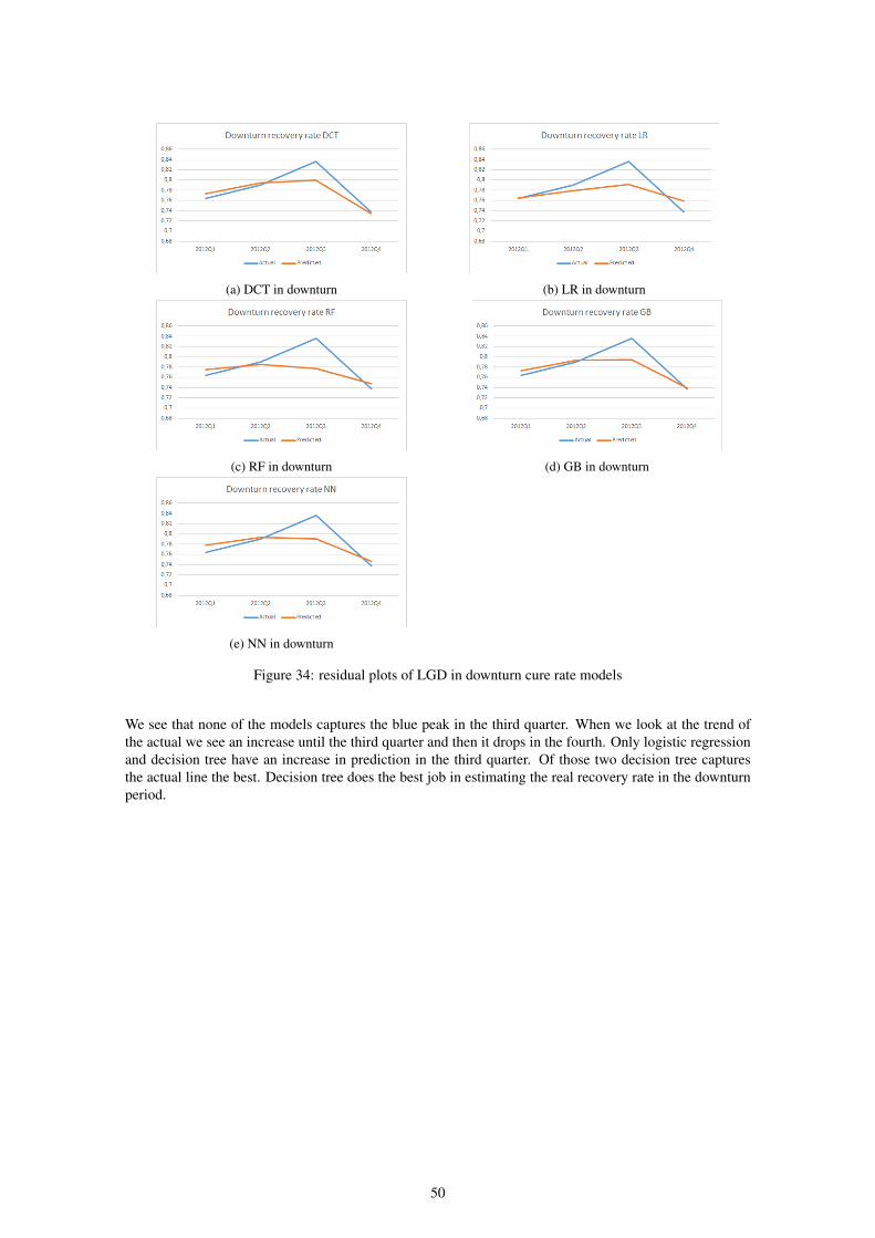
(a) DCT in downturn (b) LR in downturn

(c) RF in downturn (d) GB in downturn

(e) NN in downturn

Figure 34: residual plots of LGD in downturn cure rate models

We see that none of the models captures the blue peak in the third quarter. When we look at the trend ofthe actual we see an increase until the third quarter and then it drops in the fourth. Only logistic regressionand decision tree have an increase in prediction in the third quarter. Of those two decision tree capturesthe actual line the best. Decision tree does the best job in estimating the real recovery rate in the downturnperiod.

50

(a) DCT in default (b) LR in default

(c) RF in default (d) GB in default

(e) NN in default

Figure 35: residual plots of LGD in default recovery rate models

The plots show that every model performs well. LR and NN have bigger deviations from the actual linethan the others. It is hard to see which one is the best but if we calculate the total error we find that RF hasthe lowest error, followed by GB.

feature importance Let us have a look at the most important features for the recovery rate and the differ-ence between the three cases.

51

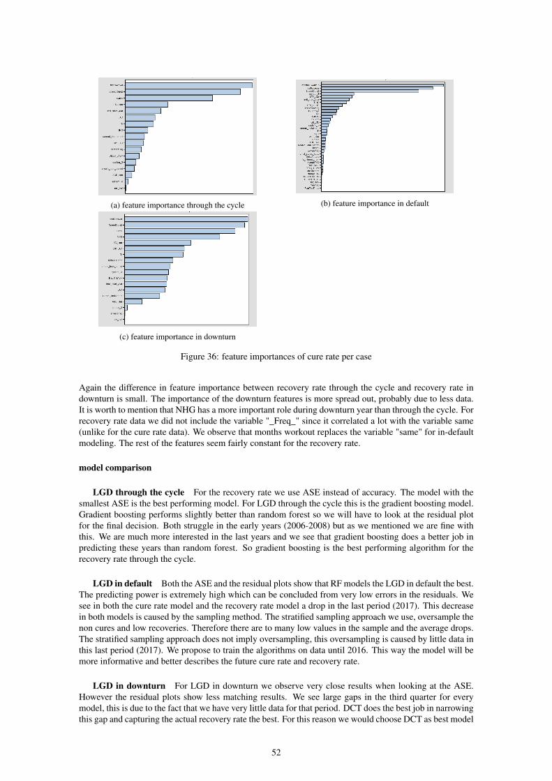
(a) feature importance through the cycle (b) feature importance in default

(c) feature importance in downturn

Figure 36: feature importances of cure rate per case

Again the difference in feature importance between recovery rate through the cycle and recovery rate indownturn is small. The importance of the downturn features is more spread out, probably due to less data.It is worth to mention that NHG has a more important role during downturn year than through the cycle. Forrecovery rate data we did not include the variable "_Freq_" since it correlated a lot with the variable same(unlike for the cure rate data). We observe that months workout replaces the variable "same" for in-defaultmodeling. The rest of the features seem fairly constant for the recovery rate.

model comparison

LGD through the cycle For the recovery rate we use ASE instead of accuracy. The model with thesmallest ASE is the best performing model. For LGD through the cycle this is the gradient boosting model.Gradient boosting performs slightly better than random forest so we will have to look at the residual plotfor the final decision. Both struggle in the early years (2006-2008) but as we mentioned we are fine withthis. We are much more interested in the last years and we see that gradient boosting does a better job inpredicting these years than random forest. So gradient boosting is the best performing algorithm for therecovery rate through the cycle.

LGD in default Both the ASE and the residual plots show that RF models the LGD in default the best.The predicting power is extremely high which can be concluded from very low errors in the residuals. Wesee in both the cure rate model and the recovery rate model a drop in the last period (2017). This decreasein both models is caused by the sampling method. The stratified sampling approach we use, oversample thenon cures and low recoveries. Therefore there are to many low values in the sample and the average drops.The stratified sampling approach does not imply oversampling, this oversampling is caused by little data inthis last period (2017). We propose to train the algorithms on data until 2016. This way the model will bemore informative and better describes the future cure rate and recovery rate.

LGD in downturn For LGD in downturn we observe very close results when looking at the ASE.However the residual plots show less matching results. We see large gaps in the third quarter for everymodel, this is due to the fact that we have very little data for that period. DCT does the best job in narrowingthis gap and capturing the actual recovery rate the best. For this reason we would choose DCT as best model

52

for the recovery rate. If we have more data for the downturn period we believe other algorithms wouldflourish more based on previous experiences and knowledge of the different algorithms.

9.3 In default adjustmentOur final experiment is to make an adjustment for the LGD in default models because they showed decreasesin averages in the last year. This change in average was due to little data in the sample set which does notrepresent the original data well. To adjust for this we cap the cure rate model at January 2017 and therecovery rate model at July 2016. These thresholds have been chosen by the amount of records we oughtednecessary to model. Both adjusted datasets will be trained by a random forest algorithm since it was thebest performing algorithm before the adjustment.

Results adjusted models The cure rate model did not change much. The misclassification rate droppedslightly from 0.084 to 0.086. The feature importance list did not alter but the weights of the features did.These weights are more informative than the weights before due to the deletion of not accurate data. Thisadjusted model is more representative for the in default cure rate than the model on the full sample set. Thenumber weighted analysis shows a slightly better plot for the adjusted model.

Figure 37: adjusted in default cure rate model RF

The recovery rate model improved by the adjustments.The ASE stayed the same 0.014 to 0.014 but the errorof the fit decreased. Interesting to observe is also the change in feature importance.

Figure 38: feature importance adjusted recovery rate model

Fastrecover rises to the most important feature, months workout and euribor3 become less important. Prob-ably the importance of the fastrecover variable interfered with the noise in the data before. This feature

53

importance list seems more reliable as it matches the recovery rate through the cycle featurelist more. Asthe error in the fit decreases the fit is also slightly better.

Figure 39: adjusted in default recovery rate model RF

9.4 Summary of resultsTo sum up the best algorithms for the six different cases:

SummaryCase Best suited algorithm

Cure rate through the cycle Random forestCure rate in default Random forest

Cure rate in downturn Neural NetworkRecovery rate through the cycle Gradient Boosting

Recovery rate in default Random ForestRecovery rate in downturn Decision Tree

Random forest dominates the table with being the best of 3 out of 6 cases. Neural network is surprising forcure rate in downturn as this algorithm usually needs lots of training data.

9.5 ScorecardsTo get a better understanding of the models and how the different features interact with the predictions ofthe cure rate and recovery rate, we generated scorecards of the best algorithms per case we just discussed.These scorecards show how the model comes to the prediction based on points. The prediction of the targetvariable is a sum of these points which are between 0 and 1000. If an observation scores 1000 points thanthe algorithm will predicts a score of 100%, vice versa if an observation scores 0 points than the algorithmpredict 0% recovery or cure. If a variable has a high feature importance this will also lead to a larger shareof points to pass out. The scorecards are in the appendix.

54

10 Discussion and ConclusionDuring this research, we modeled the Loss Given Default (LGD) under different conditions and with dif-ferent models. We first explained the background of the problem and why we are taking this new approach,also we discussed several models of this approach. Secondly, we inspected the data, cleaned the data, madea univariate analysis and transformed some variables. This was done to get a dataset for each case we areinvestigating. These datasets were used to train models to predict the two key components of the LGD for-mula (cure rate and recovery rate). Next to manipulating the data we also tuned the hyperparameters withgrid search. For in default modeling we had to use stratified sampling to get a representative dataset andfor in downturn modeling we had to decide which year to pick for downturn modeling. All these steps ledto the two experiments cure rate & recovery rate where we compared 5 models for each case to see whichperforms the best. The first goal we had, was whether the LGD could be modeled with machine learningand the second goal was to get the best performing model per case. We conclude from our research thatthe new LGD methodology, modeling based on characteristics of customers and estimating the cure rateand recovery rate with machine learning, is a promising and reliable way for banks to model their LGD.Having this said the models can be improved further and analysis could be further expanded. For instance,in the starting database of ING there were a lot of re-defaults. Most of them are filtered out but there allstill some re-defaults. If these are filtered out we have a cleaner dataset. Another data-related improvementis the increase of recovery rate in downturn data. Right now we are restricted to using 1 year of data whichis a constraint of the amount of data. If we would use multiple years this might improve predictions forthe downturn model. A couple of minor improvements could be made such as providing the feature im-portance for all algorithms instead of just random forest to gain more insight. Different ensemble methodsor machine learning techniques could be used to try to get better predictions. At last the hyperparameteroptimization for recovery rate can be improved. At the moment it is not possible to do grid search for acontinuous target variable, so the optimization was done by hand. This probably led to a local maximum ofhyperparameters settings.

55

11 References

References[1] E. Spuchlakova & J. Cug, Credit Risk and LGD modelling

[2] P Christian, Estimating Loss Given Default – Experiences from Banking Practice

[3] P. Crosbi, J.J.R. Bohn, Modelling Default Risk, Modelling Methodology

[4] D. Gorter, Added value of machine learning in retail credit risk

[5] F. Martinsson, Exotic approaches for modelling Loss Given Default

[6] Tim Slingerland, Arjen Pengen Scorecard for analytics

[7] Bill Huajian Yang and Mykola Tkachenko Modeling of EAD and LGD: Empirical Approaches andTechnical Implementation

[8] Gilles Louppe Understanding random forests, section 4 (random forests)

[9] Ben Gorman http://blog.kaggle.com/2017/01/23/a-kaggle-master-explains-gradient-boosting/

[10] Alexey Natekin, Alois Knoll Gradient boosting machines, a tutorial

[11] Min Qi, Xinlei Zhao Comparison of modeling methods for Loss Given Default

[12] Guoqiang Zhang , Michael Y. Hu , B. Eddy Patuwo , Daniel C. Indro Artificial neural networks inbankruptcy prediction: General framework and cross-validation analysis

[13] Gilles Louppe Understanding random forests, section 2.4.3 (neural networks)

[14] Prashant Gupta https://towardsdatascience.com/decision-trees-in-machine-learning-641b9c4e8052

[15] Sandro Sperandei Understanding logistic regression analysis

[16] Niklas Donges https://towardsdatascience.com/the-logistic-regression-algorithm-75fe48e21cfa

56

challenging lgd models with machine learningsbhulai/papers/thesis-severeijns.pdfchallenging lgd...

Documents