challenges facing the use of mid-range meteorological
TRANSCRIPT

PRESENTATION
Canadian Wildfire Conference, Kitchener-Waterloo Wednesday October 6th 2010
0. Abstract 1. Mathematical Theory of chaos 2. Operational mid-range ensemble model forecast
a. Canadian Ensemble models b. North-American Ensemble Forecast System
3. Quasi-deterministic Approach using ensemble models 4. Fire Meteorology: Approach versus time window
5. Proposal: Consultation working group on the use of mid-term meteorological ensemble
models to develop fire management decision tools
APPENDIX A: Ensemble Forecasting at NCEP

Mathematical Theory of Chaos Extracts from http://en.wikipedia.org/wiki/Chaos_theory Historical Background:
Chaos theory is a field of study in mathematics, physics, economics and philosophy studying the behaviour of dynamical systems that are highly sensitive to initial conditions This sensitivity is popularly referred to as the butterfly effect Small differences in initial conditions (such as those due to rounding errors in
numerical computation) yield widely diverging outcomes for chaotic systems, rendering long-term prediction impossible in general
This happens even though these systems are deterministic, meaning that their future behaviour is fully determined by their initial conditions, with no random elements involved In other words, the deterministic nature of these systems does not make them
predictable This behaviour is known as deterministic chaos, or simply chaos
Chaotic behaviour can be observed in many natural systems, such as the weather
Explanation of such behaviour may be sought through analysis of a chaotic
mathematical model, or through analytical techniques such as recurrence plots and Poincaré maps

Mathematical Theory of Chaos (2)
The main catalyst for the development of chaos theory was the electronic computer
Much of the mathematics of chaos theory involves the repeated iteration of simple
mathematical formulas, which would be impractical to do by hand Electronic computers made these repeated calculations practical, while figures and
images made it possible to visualize these systems
An early pioneer of the theory was Edward Lorenz whose interest in chaos came about accidentally through his work on weather prediction in 1961 Lorenz was using a simple digital computer He wanted to see a sequence of data again and to save time he started the simulation
in the middle of its course using the printout The computer worked with 6-digit precision, but the printout rounded variables off to
a 3-digit number, so a value like 0.506127 was printed as 0.506 This difference is tiny and the consensus at the time would have been that it should
have had practically no effect
Lorenz had discovered that small changes in initial conditions produced large changes in the long-term outcome
Lorenz's discovery, which gave its name to Lorenz attractors, showed that even detailed atmospheric modelling cannot in general make long-term weather predictions
Weather is usually predictable only about a week ahead!

Operational Mid-Range Ensemble Models Forecast
Canadian Ensemble Models (CMC) North American (NAEFS) US (NCEP)
o APPENDIX A: Reference Paper (NCEP, 1995)
Canadian ensemble forecasts http://www.weatheroffice.gc.ca/ensemble/index_e.html
The daily ensemble forecasts have been available operationally since January 24, 1996. They were originally performed with eight members. As of August 24, 1999, eight more members were added creating a 16-member ensemble forecast system. On January 12, 2005, the Optimal Interpolation Technique for the analysis cycle was replaced with the Ensemble Kalman Filter Technique. Starting in July 2007, four more members were added to produce a 20-member ensemble. Twice a day 20 "perturbed" 16-day weather forecasts are performed as well as an unperturbed 16-day control forecast. The 20 perturbed forecasts and the control forecast are performed with the GEM model. The 20 models have different physics parameterizations, data assimilation cycles and sets of perturbed observations.
500 Mb 582 dam Time series T+0 / T+120 / T+240 and T+360 Hours
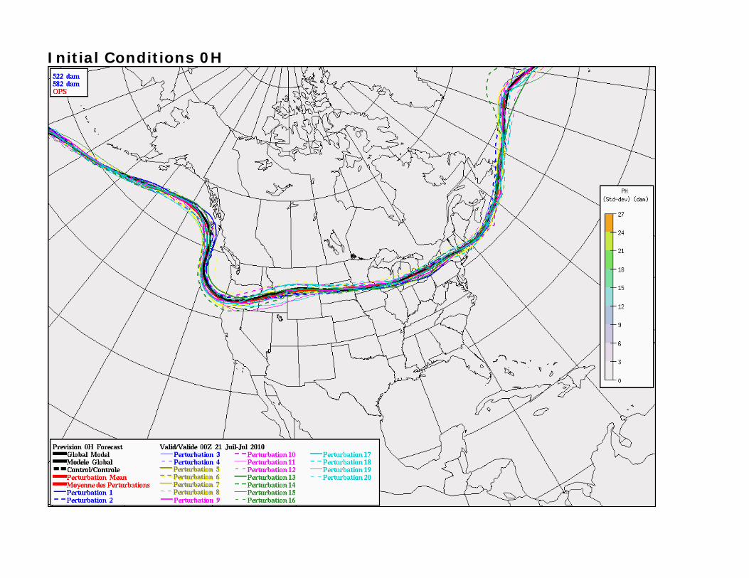
Initial Conditions 0H

Prevision: 120H
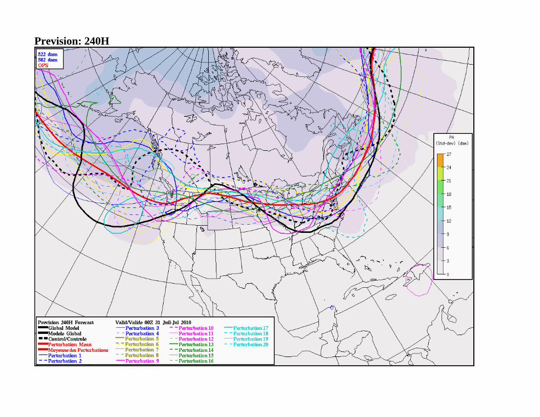
Prevision: 240H
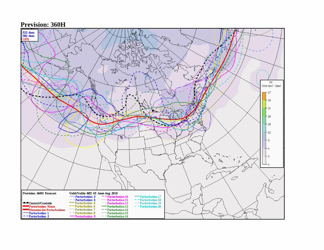
Prevision: 360H

Definition of the control model and perturbed models http://www.weatheroffice.gc.ca/ensemble/verifs/model_e.html
All members GEM model as dynamical core
Global horizontal computational grid of 400x200 points
28 levels of computation in the vertical
Control Model
Parameter for Gravity Wave Drag = 8.0e-6 m-1 (McFarlane, 1987)
ISBA type of land surface processes (Noilhan & Planton, 1989)
Sundqvist et al. (1989) type of condensation (consun)
Kain & Fritsch (1993) convective scheme
Shallow convection simulated (conres & ktrsnt_mg)
Bougeault & Lacarrère (1989) mixing length formulation
Turbulent vertical diffusion parameter (Beta) = 1.0
These are the same schemes as those used by CMC's deterministic global model
The 20 perturbed GEM models
All perturbed models use the energy back-scattering scheme (Shutts, 2005) and stochastic perturbations of the physical tendencies.

NAEFS North American Ensemble Forecast System The North American Ensemble Forecast System (NAEFS) is run at 00 and 12 UTC
each day
40 ensemble members plus two controls
o 20 members from GEFS (Global Ensemble Forecast System) at NCEP
o 20 members from CEFS (Canadian Ensemble Forecast System) at the
Canadian Meteorological Center (CMC)
US: http://www.emc.ncep.noaa.gov/gmb/ens/index.html CANADA: http://www.meteo.gc.ca/ensemble/index_f.html
http://www.weatheroffice.gc.ca/ensemble/naefs/index_e.html
Joint project involving the Meteorological Service of Canada (MSC), the United States National Weather Service (NWS) and the National Meteorological Service of Mexico
o NAEFS combines state of the art ensemble forecasts, developed at the MSC and the NWS. When combined, the grand ensemble can provide weather forecast guidance for the 1-14 day period that is of higher quality than the currently available operational guidance based on either set of ensembles alone.
o It allows the generation of a set of forecast products that are seamless across the national boundaries between Canada, the United States and Mexico.
o The research/development and operational costs of the NAEFS system are shared by the three organizations (MSC, NWS, and NMSM), which make it more cost effective and result in higher quality and more extensive weather forecast products.
Temperature Anomaly: Day 8 to 14 Outlooks EPSgrams for cities in Canada, Mexico and United States of America Ensemble means and standard deviation charts Maps of probabilities of occurrence of several weather events
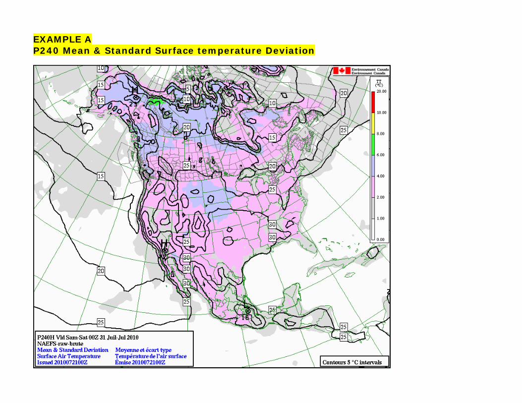
EXAMPLE A P240 Mean & Standard Surface temperature Deviation
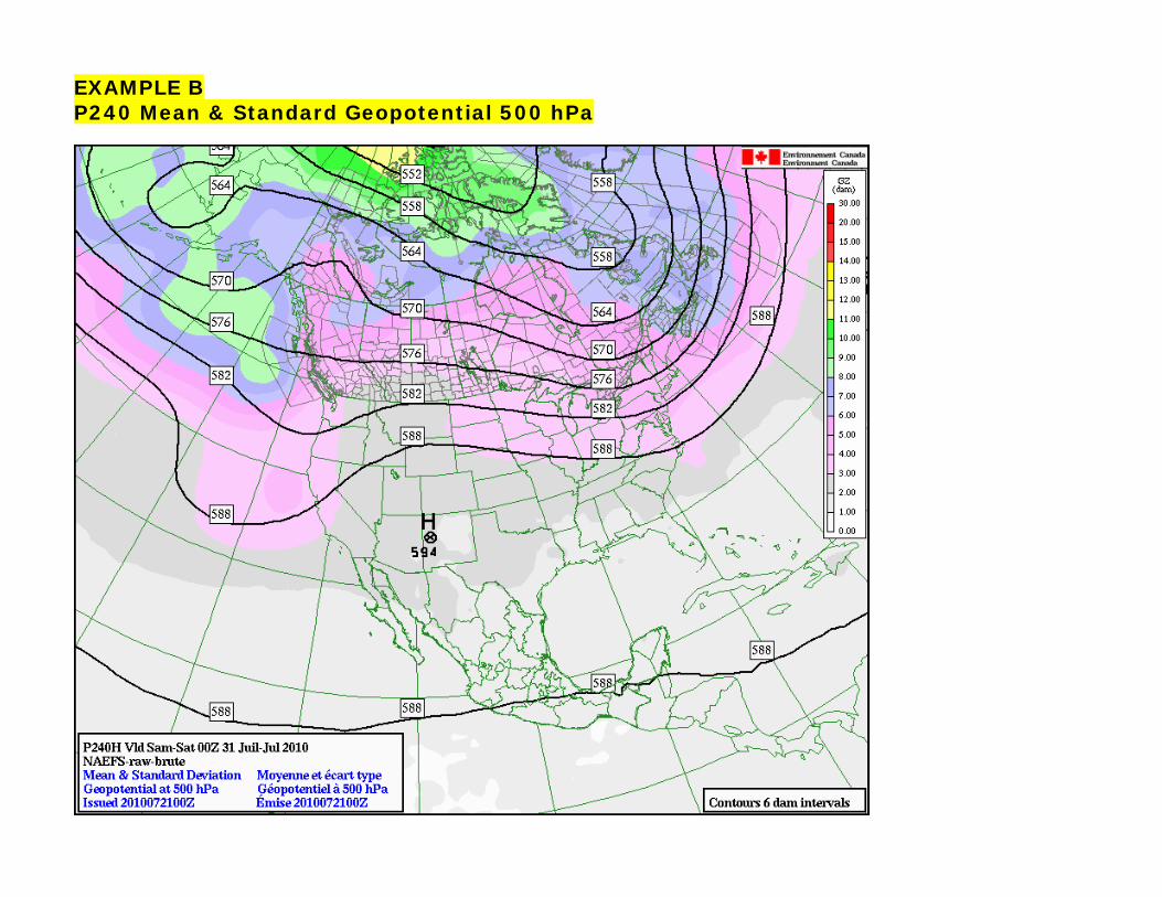
EXAMPLE B P240 Mean & Standard Geopotential 500 hPa
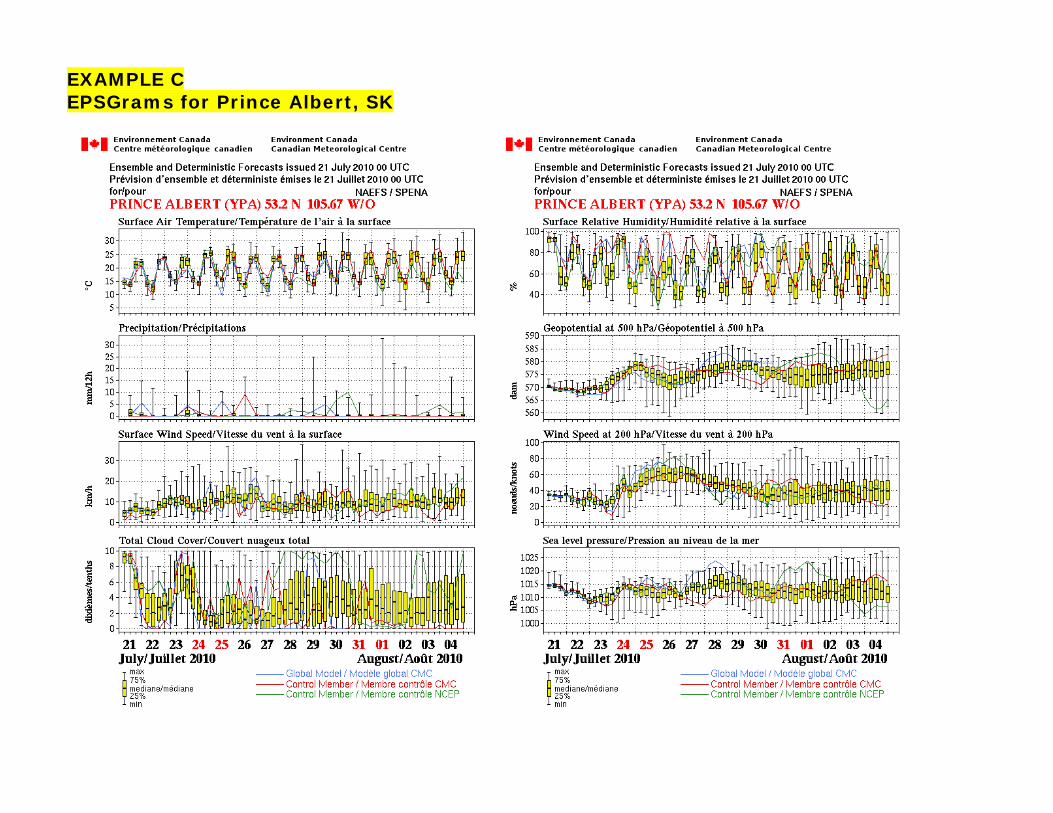
EXAMPLE C EPSGrams for Prince Albert, SK
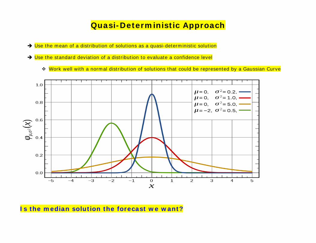
Quasi-Deterministic Approach
Use the mean of a distribution of solutions as a quasi-deterministic solution
Use the standard deviation of a distribution to evaluate a confidence level
Work well with a normal distribution of solutions that could be represented by a Gaussian Curve
Is the median solution the forecast we want?

Even if it might be the least likely outcome! Below are 5 hypothetical probabilistic scenarios
Each scenario has 40 solutions
Each graph is a Probabilistic distribution of Threat Ranking
Which ones would be best represented by a quasi-deterministic solution?
Which ones wouldn’t be?

Fire Meteorology
A Deterministic Approach work well for the first 48H A Quasi-deterministic Approach offers a transition for the 48-120H
A Probabilistic Approach for the 120-360H provides us with full spectrum of potential
solutions that are better suited to a fire management risk management decision-making model
MICROSCALE
MESOSCALE
REGIONAL
GLOBAL
MID-RANGE
SEASONAL
SHORT-CLIMATE
H+1 H+9 H+48 D+7 D+30 M+6 Y+10

In the forecasting time window of 3-15 Days
What types of forecast fire weather
fire behaviour ranks fire growth potential
Do wildland fire organizations need for decision-support tools?
Organizational potential stress
Performance expectations Human Resources Financial Political
Import-Export cost-effective risk management
Management of rotary wings contracts or fixed wings capability
Potential mid-term threat of monitored wildland fires
Priorization between wildland fires in multiple fires situation
Media communication strategy
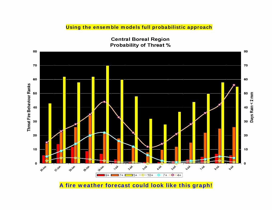
Using the ensemble models full probabilistic approach
A fire weather forecast could look like this graph!

What are the strengths and weaknesses
Of meteorological numerical models
In forecast weather elements for
Fire meteorology & fire behaviour?
Likely Strengths:
Realistic temperature & wind fields based on weather pattern predicted by each member of the ensemble
Suspected Weaknesses by most members of the ensemble models:
Relative humidity fields problematic in short term forecast due to the compromise between boundary layer moisture content and convective precipitation generation
Relative humidity field likely problematic in mid-term forecasting
Convective precipitation generation in mid-term forecasting
Realistic cumulative precipitation amounts over time
Lightning activity type predictors to evaluate dry lightning potential

Are each member of the ensemble properly weighted?
Physical parameterizations? Initializations?
Are each member as likely to be to most accurate?
In what aspects? To answer these questions…
To explore operational solutions…
To better communicate our limitations versus needs…

Consultation working group
On the use of mid-term meteorological ensemble models
To develop fire management decision tools
Proposal: Establishment of a Canadian consultation working group comprised of meteorological modelers, fire behaviour and fire meteorology experts To better communicate wildfire management needs for decision-making tools To discuss fire behaviour/fire meteorologists expectations in developing solutions
and tools to answer these needs To encourage active collaboration between experts in research and projects
development To understand limitations and challenges in providing meteorological probabilistic
solutions used as based data for these tools

Please e-mail me to express your interest …
Daniel Poirier Chief Meteorologist
Saskatchewan Environment 306-953-3439
THANK YOU

APPENDIX B http://www.emc.ncep.noaa.gov/gmb/ens/info/ens_detbak.html
ENSEMBLE FORECASTING AT NCEP (16 November 1995)
INTRODUCTION
Since the atmosphere is a chaotic dynamical system, any small error in the initial condition will lead to growing errors in the forecast, eventually leading to a total loss of any predictive information. This is so even if our models were perfect (Lorenz, 1969). The rate of this error growth and hence the lead time at which predictability is lost depends on factors such as the circulation regime, season, and geographical domain. It is possible to obtain information on the inherent predictability of a given case by running the model from a number of initial conditions that lie within the estimated cloud of uncertainty that surrounds the control analysis (which is our best estimate of the true state of the atmosphere).
In the extratropics numerical weather prediction models are good enough so that to a first approximation forecast error growth can be attributed solely to the process of growing instabilities in a chaotic system that result from initial condition uncertainties. In our current ensemble approach, therefore, we assume that our models are "perfect" and introduce perturbations only to the analysis (rather than or in addition to, for example, perturbations in model physics).
The above described role of chaos is evident on all spatial and temporal scales in the atmosphere and ocean. So, ideally, all forecasts should be made from an ensemble of initial conditions. In fact in any nonlinear dynamical system this approach offers the best possible forecast with the maximum information content. Averaging the ensemble members provides in a statistical sense a forecast more reliable than any of the single forecasts, including that started from the control analysis (Leith, 1974). Additionally, from the spread of the ensemble we can assess the reliability of the predictions and, for a sufficiently large number of realizations, any forecast quantity can be expressed in terms of probabilities. These probabilities convey all the information available regarding future weather. Note that each individual model run is deterministic, i.e., uniquely defined by the initial conditions, but collectively the ensemble of forecasts from the set of slightly different analyses portrays the chaotic nature of the atmosphere. Since a priori any single ensemble member is no more or less likely than any other, forecasting can be viewed as deterministic only to the extent that the envelope of solutions is sufficiently small that the differences between forecasts are inconsequential to the user. Otherwise, the variety

of solutions and the implied uncertainty reflect the more general stochastic nature of the forecast process, with the range and distribution of possible outcomes providing information on the relative likelihood of various scenarios.
At NCEP the ensemble approach has been applied operationally for the medium- and extended range (Tracton and Kalnay, 1993; Toth and Kalnay, 1993), using the Environmental Modeling Center's (EMC) Medium-Range Forecast Model (MRF), which has a global domain. This document contains information regarding the operational global ensemble forecasts. However, short-range ensemble forecasts are also created at NCEP on an experimental basis, using the ETA and Regional Spectral Models (Brooks et al., 1995; Hamill and Collucci, 1996). Planning is also underway to run the coupled ocean- atmosphere model of EMC in an ensemble mode (Toth and Kalnay, 1995).
THE ENSEMBLE FORECAST SYSTEM:
MODEL CONFIGURATION
There will always be a trade-off between the resolution at which the forecasts are made and the number of ensemble forecast members, due to limited computational resources. Since the impact of using a higher resolution model is not detectable with traditional skill scores beyond a few days (Tracton and Kalnay, 1993), at NCEP we truncate the resolution of the nominal MRF and AVN runs (T126 truncation, ~100 km) to T62 (~200 km) at a lead times of 7 and 3 days at 00Z and 12Z, respectively. At 00Z there is also a "control" totally T62 run. In addition to this control forecast, 10 forecasts with T62 resolution are run from 00Z starting from slightly perturbed initial conditions. At 12Z four additional forecasts are generated from perturbed initial analyses. Hence, there is a total of 17 individual global predictions generated daily. All forecasts are run to 16 days with the latest version of the EMC MRF global model (Kanamitsu et al., 1993). Evaluations indicate that for the first week or so for daily forecasts, the set of 17 ensemble members is sufficient. For the currently operational 6-10 day mean outlooks (and future "week2" forecasts), additional information is added by including the runs from up to 48 hours prior to "todays" 00Z set in the time (or lagged) average sense (Hoffman and Kalnay, 198*). In this application the total the number of forecasts (ensemble size) equals 46.
INITIAL PERTURBATIONS
There has been considerable effort directed at the question of optimal initial perturbations. There are two major considerations. The first is to estimate the analysis error in the probabilistic sense, and the second is to create an adequate sampling of perturbations given this statistical estimate of initial uncertainty. Since not all errors in the analysis are likely to grow, adequate here encompasses not just the question of representativeness. It includes also the notion of economy in identifying only those initial uncertainties that result in rapidly diverging solutions (e.g., errors in analysis of a baroclinic zone versus those in a broad ridge).

If the analysis error had a white noise distribution (i. e., all possible analysis errors occurred with the same probability), the best sampling strategy would be the use of the singular vectors (SVs) of the linear tangent version of the nonlinear model (Buizza and Palmer, 199*; Ehrendorfer and Tribbia, 1995). This is because the leading SVs span those directions in the phase space that are capable of maximum error growth. If we miss those directions, "truth" could lie outside the ensemble envelope.
The analysis error distribution, however, is far from being white noise (Kalnay and Toth, 1994): Consider the analysis/forecast cycle of the data assimilation system as running a nonlinear perturbation model. The error in the first guess (short-range forecast) is the perturbation which is periodically "rescaled" at each analysis time by blending observations with the guess. Since observations are generally sparse they can not eliminate all errors from the short-range forecast that is subsequently generated as the first guess for the next analysis. Obviously, any error that grew in the previous short-range forecast will have a larger chance of remaining (at least partially) in the latest analysis than errors that had decayed. These growing errors will then start amplifying quickly again in the next short-range forecast.
It follows that the analysis contains fast growing errors that are dynamically created by the repetitive use of the model to create the first guess fields. This is what we refer to as the "breeding cycle" or Breeding of Growing Modes (BGM). These fast growing errors are above and beyond the traditionally recognized random errors that result from errors in observations. Those errors generally do not grow rapidly since they are not organized dynamically. It turns out that the growing errors in the analysis are related to the local Lyapunov vectors of the atmosphere (which are mathematical phase space directions that can grow fastest in a sustainable manner). Indeed, these vectors are what is estimated by the breeding method (Toth and Kalnay, 1993, 1995).
At NCEP we use 7 independent breeding cycles to generate the 14 initial ensemble perturbations. The initiation of each breeding cycle begins with an analysis/forecast cycle which differs from the others only in the initially prescribed random distribution ("seed") of analysis errors. These initially random perturbations are added and subtracted from the control analysis, so that each breeding cycle generates a pair of perturbed analyses (14 in all). From this point on each breeding cycle evolves independently to produce its own set of perturbations. The perturbations are just the differences between the short-term forecast (24 hour) initiated from the last perturbed analysis and the "control" analysis, rescaled to the magnitude of the seed perturbation. Since these short-term forecasts are just the early part of the extended range ensemble predictions, generation of the perturbations is basically cost free with respect to the analysis system (unlike the singular vector approach of ECMWF). The cycling of the perturbations continues and within a few days the perturbations reach their maximum growth.
Note that once the initial perturbations are introduced, the perturbation patterns evolve freely in the breeding cycle except that their size is kept within a certain amplitude range. Also note the similarity in the manner errors grow in the analysis vs. breeding cycles. The only difference is that from the breeding cycle, the stochastic elements that are introduced into the analysis through the use of observations containing random noise are eliminated by the use of deterministic rescaling. The
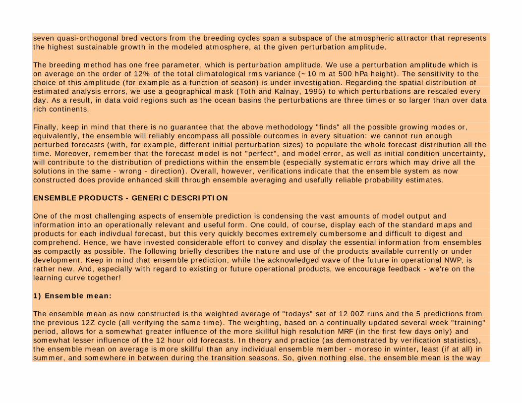
seven quasi-orthogonal bred vectors from the breeding cycles span a subspace of the atmospheric attractor that represents the highest sustainable growth in the modeled atmosphere, at the given perturbation amplitude.
The breeding method has one free parameter, which is perturbation amplitude. We use a perturbation amplitude which is on average on the order of 12% of the total climatological rms variance (~10 m at 500 hPa height). The sensitivity to the choice of this amplitude (for example as a function of season) is under investigation. Regarding the spatial distribution of estimated analysis errors, we use a geographical mask (Toth and Kalnay, 1995) to which perturbations are rescaled every day. As a result, in data void regions such as the ocean basins the perturbations are three times or so larger than over data rich continents.
Finally, keep in mind that there is no guarantee that the above methodology "finds" all the possible growing modes or, equivalently, the ensemble will reliably encompass all possible outcomes in every situation: we cannot run enough perturbed forecasts (with, for example, different initial perturbation sizes) to populate the whole forecast distribution all the time. Moreover, remember that the forecast model is not "perfect", and model error, as well as initial condition uncertainty, will contribute to the distribution of predictions within the ensemble (especially systematic errors which may drive all the solutions in the same - wrong - direction). Overall, however, verifications indicate that the ensemble system as now constructed does provide enhanced skill through ensemble averaging and usefully reliable probability estimates.
ENSEMBLE PRODUCTS - GENERIC DESCRIPTION
One of the most challenging aspects of ensemble prediction is condensing the vast amounts of model output and information into an operationally relevant and useful form. One could, of course, display each of the standard maps and products for each indivdual forecast, but this very quickly becomes extremely cumbersome and difficult to digest and comprehend. Hence, we have invested considerable effort to convey and display the essential information from ensembles as compactly as possible. The following briefly describes the nature and use of the products available currently or under development. Keep in mind that ensemble prediction, while the acknowledged wave of the future in operational NWP, is rather new. And, especially with regard to existing or future operational products, we encourage feedback - we're on the learning curve together!
1) Ensemble mean:
The ensemble mean as now constructed is the weighted average of "todays" set of 12 00Z runs and the 5 predictions from the previous 12Z cycle (all verifying the same time). The weighting, based on a continually updated several week "training" period, allows for a somewhat greater influence of the more skillful high resolution MRF (in the first few days only) and somewhat lesser influence of the 12 hour old forecasts. In theory and practice (as demonstrated by verification statistics), the ensemble mean on average is more skillful than any individual ensemble member - moreso in winter, least (if at all) in summer, and somewhere in between during the transition seasons. So, given nothing else, the ensemble mean is the way

to go. The ensemble mean will usually be "smoother" in appearance than any of the individual forecasts because the averaging filters the "unpredictable components", where unpredictable here means inconsistencies amongst ensemble members. Conceptually, considering anything with more detail than contained in the ensemble mean over specifies the inherent predictability; however, note that, if most of the ensemble members are similar in the amplitude and phase of even smaller-scale features, they will be retained in the ensemble mean.
2) Ensemble Spread:
The ensemble mean is just the first order advantage of ensemble prediction. Its more significant use is in providing information on uncertainties and/or confidence. The most basic product addressing this is the ensemble spread, which here is simply the standard deviation of the ensemble members about the ensemble mean. It reflects the overall degree of variability amongst the ensemble members - the larger values indicating areas of substantial disagreement and hence less confidence in any individual prediction (or ensemble mean) and visa versa. The maps of spread thus provide an evolving measure of the relative confidence geographically and with respect to individual weather systems.
3) Clustering:
Clustering here refers to grouping together ensemble members that are similar in some respect. The approach used here is based on simple correlation analysis. First, the two predictions least similar (smallest anomaly correlation < 0.6) are determined. Ensemble members similar (AC>0.6) to each of these extremes (if any) are found, and the cluster mean for each formed. Unless no two forecasts are dissimilar there will always be at least two clusters (C1, C2), possibly consisting of only one forecast each, which correspond to the range of solutions sampled by the ensemble. Second, of the remaining forecasts, the two most similar are found, and members similar to them grouped (averaged) to form the next cluster. The process iterates until there is no longer any set of at least two forecasts that are similar (maximum of 6 allowed). The cluster means effectively reduce the number of degrees of freedom relative to considering the complete set of individual forecasts, but not so much as the full ensemble mean (except if all the forecasts are alike). Ideally, and for the most part as indicated by verification scores, the more populated a cluster the more skillful the cluster mean.
Currently, the only two fields clustered are the 1000 and 500 mb height fields. Clustering is relative to the similarities amongst forecasts averaged over North American and its environs. The specifics of the domain are given in the detailed documentation. In the future we expect to perform the clustering for smaller sub regions and for other fields (ultimately, we hope, to be selected interactively by the forecaster). Also at present the clustering is done independently by level and time, so that the cluster membership at a given time may be different for 1000 and 500 mb and for either level different from one forecast time to the next. An alternative approach (available in the near future) is to force the cluster membership for all times and for each level to that determined for 500mb at day 5. While this will allow tracing the evolution of each ensemble over time with assurance that membership is unchanging, it may or may not be a better approach; forecasts similar at, for example day 3, may quite naturally diverge and be similar to members by day 6 they had little in common with earlier. (Clustering relative to mean conditions, e.g., days 3-5, have not proved satisfactory at ECMWF.)
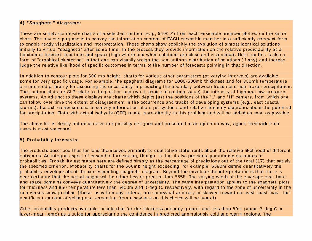
4) "Spaghetti" diagrams:
These are simply composite charts of a selected contour (e.g., 5400 Z) from each ensemble member plotted on the same chart. The obvious purpose is to convey the information content of EACH ensemble member in a sufficiently compact form to enable ready visualization and interpretation. These charts show explicitly the evolution of almost identical solutions initially to virtual "spaghetti" after some time. In the process they provide information on the relative predictability as a function of forecast lead time and space (high where and when solutions are close and visa versa). Note too this is also a form of "graphical clustering" in that one can visually weigh the non-uniform distribution of solutions (if any) and thereby judge the relative likelihood of specific outcomes in terms of the number of forecasts pointing in that direction.
In addition to contour plots for 500 mb height, charts for various other parameters (at varying intervals) are available, some for very specific usage. For example, the spaghetti diagrams for 1000-500mb thickness and for 850mb temperature are intended primarily for assessing the uncertainty in predicting the boundary between frozen and non-frozen precipitation. The contour plots for SLP relate to the position and (w.r.t. choice of contour value) the intensity of high and low pressure systems. An adjunct to these displays are charts which depict just the positions of the "L" and "H" centers, from which one can follow over time the extent of disagreement in the occurrence and tracks of developing systems (e.g., east coastal storms). Isotach composite charts convey information about jet systems and relative humidity diagrams about the potential for precipitation. Plots with actual isohyets (QPF) relate more directly to this problem and will be added as soon as possible.
The above list is clearly not exhaustive nor possibly designed and presented in an optimum way; again, feedback from users is most welcome!
5) Probability forecasts:
The products described thus far lend themselves primarily to qualitative statements about the relative likelihood of different outcomes. An integral aspect of ensemble forecasting, though, is that it also provides quantitative estimates of probabilities. Probability estimates here are defined simply as the percentage of predictions out of the total (17) that satisfy the specified criterion. Probability charts for the 500mb height exceeding, for example, 5580m define quantitatively the probability envelope about the corresponding spaghetti diagram. Beyond the envelope the interpretation is that there is near certainty that the actual height will be either less or greater than 5558. The varying width of the envelope over time and space domains conveys quantitatively the degree of uncertainty. The same interpretation applies to the spaghetti plots for thickness and 850 temperature less than 5400m and 0-deg C, respectively, with regard to the zone of uncertainty in the rain versus snow problem (these, as with many criteria, are somewhat arbitrary or skewed toward our east coast bias - but a sufficient amount of yelling and screaming from elsewhere on this choice will be heard!).
Other probability products available include that for the thickness anomaly greater and less than 60m (about 3-deg C in layer-mean temp) as a guide for appreciating the confidence in predicted anomalously cold and warm regions. The

probability of 700mb RH > 70% can be considered a proxy for precipitation chances, which will be added explicitly in the near future. The predicted odds for the 12hr 500 height tendency > 30m chart is an indicator of the degree of consistency amongst the members in depicting short-wave activity; consistency in treatment of the smaller-scale systems (because they are intrinsically less predictable) is a signal to take the implications seriously. In principle probability information on any direct or derived model parameter can be output - so let your requests come forward (how about vertical stability or indices such as the PNA?). Another form of probability chart, currently being developed, is to express the confidence in percentages of, for example, the 850mb temperature anomaly being within 5-deg of the ensemble mean value (or any other base for comparison).
A final few words on ensemble derived probabilities. Many forecasters have come to know and use (and love?) probability statements for precipitation and temperature. These generally are the direct or somewhat modified POP's and POT's generated statistically by TDL via the MOS (or similar) approach. They basically describe the probability distributions given the parameters (or, more generally, the synoptic features) from a single (i.e., deterministic) prediction (NGM or MRF). The actual uncertainty consists of two components; that associated with the non-unique distribution of precipitation or temperature given a particular synoptic scenario AND that intrinsic to there being an array of alternative scenarios. MOS accounts now only for the first component while the probabilities derived from the direct model output (as described above) from ensembles include both. Of course, one could derive and combine precipitation and temperature probability distributions from each ensemble member, and TDL is actively pursuing this approach.

Abstract
Challenges facing the use of Mid-range meteorological ensemble models to develop wildland fire management decision-supporting tools
Daniel Poirier Daniel Poirier, Chief Meteorologist at Saskatchewan Environment has managed the weather program at Fire & Forest Protection Branch since 1999. He has worked as an operational meteorologist for Environment Canada from 1980 to 1998. He has a degree in physics from the University of Montreal, a degree in atmospheric sciences from the University of Quebec in Montreal, and a degree in education from the University of Quebec in Abitibi-Temiscamingue. Abstract: This discussion will be presented to a wider audience of wildfire meteorologists, fire behaviour researchers, numerical modelers, and wildland fire managers. The presentation will briefly note the advent and now availability of ensemble models that focus on the Days 3-15 mid-range forecasting window. It will focus on the potential these ensemble models offer in risk management and wildfire organization decision-making processes. It will note the danger in simplifying the range of scenarios they offered to emulate present day deterministic approach. It will suggest that doing so will neglect the full potential of the information provided. The presentation will ask pertinent questions regarding the weaknesses these models have in forecasting some weather elements that ultimately could lead to a tilted evaluation of the fire behaviour risk involved. It will also offer the view that collaboration between agencies would be crucial in determining the standards of the future, believing that this radical new way in visioning what a weather forecast should look like would come sooner rather than later. SUMMARY:
This discussion paper briefly mentions the advent of the mathematical chaos theory that ultimately has lead, in the last few years, to the availability in real time of mid-term meteorological ensemble models by most national or supra-
national meteorological prediction centres. This discussion papers indicates that we presently experiencing the infancy of a great scientific leap in the potentials, ways and opportunities this approach offers in improving risk management and decision-making processes in numerous fields of application such as agriculture, transportation, health and wildfire management.
Traditionally and due to the technological limitations of super computer in delivering timely numerically derived weather forecast, deterministic solutions were offered and integrated to wildfire management decision tools such as the FWI and later the FBP systems. These deterministic solutions, i.e. unique solutions for specific sites or narrow ranges for an area, were either directly numerically derived, climatologically statistically tweaked, or human adjusted. Typically, the reliability of the forecast decreases with time and this approach is still widely operationally used in the Days 0-3 short-range forecast window. Later more numerical model solutions were offered, each with their advantages and weaknesses. Gradually some deterministic solutions extended in the Days 3-10 mid-range forecasting window. While individual deterministic solutions were better than none, serious forecast reliability issues were noted.
This advance in numerical modeling and the application of new mathematics now offer the availability of probabilistic solutions that better reflect the risks associated with different weather scenarios that could impact a wildfire management organization and offer risk weighted cost-effective adaptive or palliative solutions.
Some decisions-support tools in development already explore the power offered by this new approach. I should be
noted however that some of them shrank the full spectrum of solutions to a Gaussian distributional ensemble offering the median as a quasi-deterministic solution and the standard deviation as a confidence rating. It is imperative to remember that the range of solutions offered by an ensemble of numerical models do not necessarily fit the normal distribution premises and in that in some cases the median solution might be the least likely outcome.
Another drawback is that these tools might focus on the prediction of the weather elements and not their combined
effects on ignition, fire behaviour potential or fire growth potentials. Most wildland fire organizations have developed and now operationally use indexes that better reflect the fire behavior threat and the potential load on their organization capacity. In Canada, all these indexes are fire weather based and in some cases reflect the fire behaviour associated with their dominant fuel. Their policies in regard to preparedness and suppression commitments are usually tied to the range of these indexes. In Saskatchewan the Preparedness levels are directly associated to ranges of HFI values in C2 fuel environment.
Meteorological numerical models have been known since their inception to be particularly weak in forecasting
moisture in the boundary layer near the surface, i.e. in forecasting dew points and its derivative relative humidity. This is still the case today in Days 0-5 short-range to mid-range forecasting window especially during the spring and summer season. It has been noted that while it is possible to improve a model performance on this particular weakness, it usually leads to less realistic convection generation and ultimately less realistic summer precipitation regime. It is a reality that mathematical schemes used by most of today’s numerical models offered a balance between these two tendencies while respecting the model time-step stability the furthest in the forecasting time window. A question has always came to mind: would it be better to use predicted weather elements originating from models with different physics, some better at representing boundary layer moisture regime, others at other physical processes such as vertical movement, etc?
Days 3-15 mid-range ensemble models typically run on a cruder grid than the higher resolution shorter-range
models. It would be crucial to evaluate first their performance, not in the specific precision of their forecast at specific locations, but on the range of weather elements solutions over the time period. Do they generate realistic range of accumulated precipitation over an area over the period? Do they have a systematic or random relative humidity bias, especially in dry regimes? These questions and more are crucial in determining these models usefulness in generating spectrum of fire behaviour values that depend on cumulative values based on the FWI system. In the coming 10 to 20 years, important developments will occur in the use of weather forecast specific to the Days 3-15 mid-range frame. This impact will radically change the ways we envision what a weather forecast look like. This will occur in wildfire weather forecasting as well. The links and integration between numerical modeling and fire weather/behaviour index systems would be based on studies and tools developed in the coming decade. Some methodology standards will be develop. In is my opinion that the weather forecast would look more like series of diagrams that would reflect risks of ignition, lightning potentials, spectrum of fire behaviour potential, availability of resources for export versus capacity needs, etc. These developments in weather forecasting applied to wildfire meteorology will necessitate a closer collaboration between the Canadian Meteorological Centre, Canadian Forest Services, Academia and operational scientist and programmers from Canadian wildfire agencies. It is time to ask today’s question: Should we form an active consultation working group dedicated to the issues regarding the mid-range forecasting to better develop the tools of tomorrow in supporting wildfire management?