Boyce/D

iPrim

a 9th

ed, C

h 7.5: H

omogen

eous

Lin

ear System

s with

Con

stant C

oefficients

Elem

entary Differential E

quations and Boundary V

alue Problem

s, 9thedition, by W

illiam E

. Boyce and R

ichard C. D

iPrim

a, ©2009 by John W

iley & S

ons, Inc.

We consider here a hom

ogeneous system of n

first order linear equations w

ith constant, real coefficients:

This system

can be written as x'=

Ax, w

here

nnn

nn

n

nn

nn

xa

xa

xa

x

xa

xa

xa

x

xa

xa

xa

x

22

11

22

221

212

12

121

111

nnn

n

n n

ma

aa

aa

a

aa

a

tx

tx

tx

t

21

222

21

112

11

2 1

,

)(

)(

)(

)(

Ax

Equilibrium

Solutions

Note that if n

= 1, then the system

reduces to

Recall that x

= 0 is the only equilibrium

solution if a

0.

Further, x

= 0 is an asym

ptotically stable solution if a<

0, since other solutions approach x

= 0 in this case.

Also, x

= 0 is an unstable solution if a

> 0, since other

solutions depart from x

= 0 in this case.

For n

> 1, equilibrium

solutions are similarly found by

solving Ax

= 0. W

e assume detA

0, so that x

= 0

is the only solution. D

etermining w

hether x=

0is asym

ptotically stable or unstable is an im

portant question here as well.

ate

tx

axx

)

(

Phase P

lane

When n

= 2, then the system

reduces to

This case can be visualized in the x

1 x2 -plane, w

hich is called the p

hase p

lane.

In the phase plane, a direction field can be obtained by evaluating A

xat m

any points and plotting the resulting vectors, w

hich will be tangent to solution vectors.

A plot that show

s representative solution trajectories is called a p

hase portrait.

Exam

ples of phase planes, directions fields and phase portraits w

ill be given later in this section.

222

121

2

212

111

1

xa

xa

x

xa

xa

x

Solving H

omogeneous S

ystem

To construct a general solution to x'=

Ax, assum

e a solution of the form

x=

ert, w

here the exponent rand the constant

vector are to be determ

ined.

Substituting x

= e

rtinto x'= A

x, we obtain

Thus to solve the hom

ogeneous system of differential

equations x'= A

x, we m

ust find the eigenvalues and eigenvectors of A

.

Therefore x

= e

rtis a solution of x'= A

xprovided that r

is an eigenvalue and

is an eigenvector of the coefficient m

atrix A.

0ξ

IA

Aξ

ξAξ

ξ

r

re

er

rtrt

Exam

ple 1: Direction F

ield (1 of 9)

Consider the hom

ogeneous equation x'= A

xbelow

.

A direction field for this system

is given below.

Substituting x

= e

rtin for x, and rewriting system

as

(A-rI)

= 0, w

e obtain

xx

1

4

11

0 0

14

11

1 1

r

r

Exam

ple 1: Eigenvalues (2 of 9)

Our solution has the form

x=

ert, w

here rand

are found by solving

Recalling that this is an eigenvalue problem

, we determ

ine rby solving det(A

-rI) = 0:

Thus r

1=

3 and r2

= -1.

0 0

14

11

1 1

r

r

)1)(

3(

32

4)

1(1

4

11

22

r

rr

rr

r

r

Exam

ple 1: First E

igenvector (3 of 9)

Eigenvector for r

1=

3:S

olve

by row reducing the augm

ented matrix:

0 0

24

12

0 0

31

4

13

1

2 1

2 1

0ξ

IA

r

2 1choose

arbitrary,

1 2/1

2/1

00

02/

11

00

0

02/

11

02

4

02/

11

02

4

01

2

)1(

2 2)1

(

2 21

ξξ

cc

Exam

ple 1: Second E

igenvector (4 of 9)

Eigenvector for r

2=

-1:S

olve

by row reducing the augm

ented matrix:

0 0

24

12

0 0

11

4

11

1

2 1

2 1

0ξ

IA

r

2 1choose

arbitrary,

1

2/1

2/1

00

02/

11

00

0

02/

11

02

4

02/

11

02

4

01

2

)2(

2 2)2

(

2 21

ξξ

cc

Exam

ple 1: General S

olution (5 of 9)

The corresponding solutions x

= e

rtof x'= A

xare

The W

ronskian of these two solutions is

Thus x

(1)and x(2)are fundam

ental solutions, and the general solution of x'=

Ax

is

tt

et

et

2 1

)(

,2 1

)(

)2(

3)1

(x

x

04

22

)(

,2

3 3)2

()1

(

t

tt

tt

ee

e

ee

tW

xx

tt

ec

ec

tc

tc

t

2 1

2 1

)(

)(

)(

23

1

)2(

2)1

(1

xx

x

Exam

ple 1: Phase P

lane for x(1)

(6 of 9)

To visualize solution, consider first x =

c1 x

(1):

Now

Thus x

(1)lies along the straight line x2

= 2x

1 , which is the line

through origin in direction of first eigenvector (1)

If solution is trajectory of particle, with position given by

(x1 , x

2 ), then it is in Q1 w

hen c1

> 0, and in Q

3 when c

1<

0.

In either case, particle moves aw

ay from origin as tincreases.

tt

te

cx

ec

xe

cx x

t3

12

31

13

12 1

)1(

2,

2 1)

(

x

12

1 2

1 13

31

23

11

22

2,

xx

c x

c xe

ec

xe

cx

tt

t

Exam

ple 1: Phase P

lane for x(2)

(7 of 9)

Next, consider x =

c2 x

(2):

Then x

(2)lies along the straight line x2

= -2x

1 , which is the

line through origin in direction of 2nd eigenvector (2)

If solution is trajectory of particle, with position given by

(x1 , x

2 ), then it is in Q4 w

hen c2

> 0, and in Q

2 when c

2<

0.

In either case, particle moves tow

ards origin as tincreases.

tt

te

cx

ec

xe

cx x

t

2

22

12

2 1)2

(2

,2 1

)(

x

Exam

ple 1: P

hase Plane for G

eneral Solution (8 of 9)

The general solution is x =

c1 x

(1)+c

2 x(2):

As t

, c

1 x(1)is dom

inantand c2 x

(2)becomes negligible.

Thus, for c

1 0,all solutions asym

ptotically approach the line x

2=

2x1

as t

.

Sim

ilarly, for c2

0,all solutions asymptotically approach

the line x2

= -2x

1as t

-.

The origin is a sad

dle p

oint,

and is unstable. See graph.

tt

ec

ec

t

2 1

2 1)

(2

31

x

Exam

ple 1: T

ime P

lots for General S

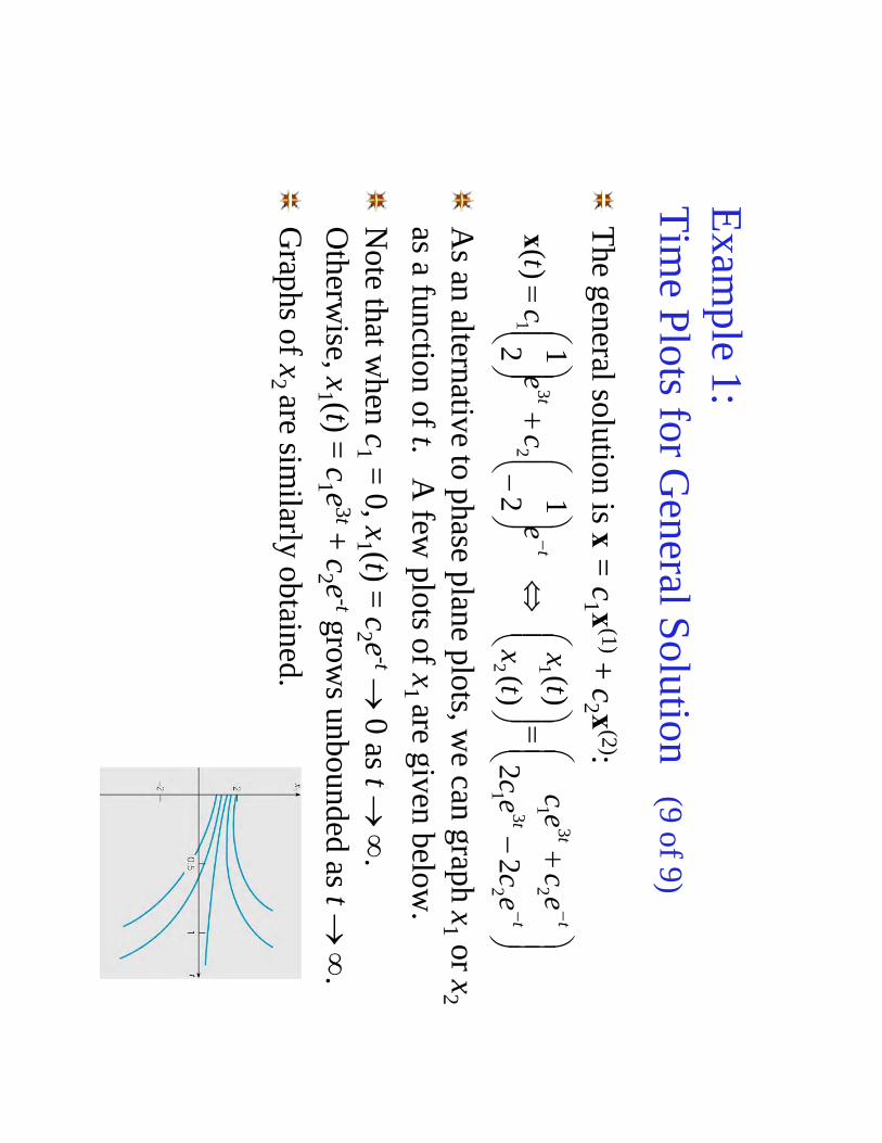
olution (9 of 9)

The general solution is x =

c1 x

(1)+c

2 x(2):

As an alternative to phase plane plots, w

e can graph x1

or x2

as a function of t. A few

plots of x1 are given below

.

Note that w

hen c1

= 0, x

1 (t) = c

2 e-t

0 as t

. O

therwise, x

1 (t) = c

1 e3t+

c2 e

-tgrows unbounded as t

.

Graphs of x

2 are similarly obtained.

tt

tt

tt

ec

ec

ec

ec

tx

tx

ec

ec

t2

31

23

1

2 12

31

22

)(

)(

2 1

2 1)

(x

Exam

ple 2: Direction F

ield (1 of 9)

Consider the hom

ogeneous equation x'= A

xbelow

.

A direction field for this system

is given below.

Substituting x

= e

rtin for x, and rewriting system

as

(A-rI)

= 0, w

e obtain

xx

2

2

23

0 0

22

23

1 1

r

r

Exam

ple 2: Eigenvalues (2 of 9)

Our solution has the form

x=

ert, w

here rand

are found by solving

Recalling that this is an eigenvalue problem

, we determ

ine rby solving det(A

-rI) = 0:

Thus r

1=

-1 and r2

= -4.

)4)(

1(

45

2)

2)(

3(

22

23

2

r

rr

rr

rr

r

0 0

22

23

1 1

r

r

Exam

ple 2: First E

igenvector (3 of 9)

Eigenvector for r

1=

-1:S

olve

by row reducing the augm

ented matrix:

0 0

12

22

0 0

12

2

21

3

2 1

2 1

0ξ

IA

r

2 1choose

2/2

00

0

02/

21

01

2

02/

21

01

2

02

2

)1(

2 2)1

(ξ

ξ

Exam

ple 2: Second E

igenvector (4 of 9)

Eigenvector for r

2=

-4:S

olve

by row reducing the augm

ented matrix:

0 0

22

21

0 0

42

2

24

3

2 1

2 1

0ξ

IA

r

1 2choose

2

00

0

02

1

02

2

02

1

)2(

2 2)

2(

ξ

ξ

Exam

ple 2: General S

olution (5 of 9)

The corresponding solutions x

= e

rtof x'= A

xare

The W

ronskian of these two solutions is

Thus x

(1)and x(2)are fundam

ental solutions, and the general solution of x'=

Ax

is

tt

et

et

4)2

()1

(

1 2)

(,

2 1)

(

xx

0

32

2)

(,

5

4 4)

2()1

(

t

tt

tt

ee

e

ee

tW

xx

tt

ec

ec

tc

tc

t

42

1

)2(

2)1

(1

1 2

2 1

)(

)(

)(

xx

x

Exam

ple 2: Phase P

lane for x(1)

(6 of 9)

To visualize solution, consider first x =

c1 x

(1):

Now

Thus x

(1)lies along the straight line x2

= 2

½x

1 , which is the

line through origin in direction of first eigenvector (1)

If solution is trajectory of particle, with position given by

(x1 , x

2 ), then it is in Q1 w

hen c1

> 0, and in Q

3 when c

1<

0.

In either case, particle moves tow

ards origin as tincreases.

tt

te

cx

ec

xe

cx x

t

12

11

12 1

)1(

2,

2 1)

(x

12

1

2

1 11

21

12

22

,x

xc

x

c xe

ec

xe

cx

tt

t

Exam

ple 2: Phase P

lane for x(2)

(7 of 9)

Next, consider x =

c2 x

(2):

Then x

(2)lies along the straight line x2

= -2

½x

1 , which is the

line through origin in direction of 2nd eigenvector (2)

If solution is trajectory of particle, with position given by

(x1 , x

2 ), then it is in Q4 w

hen c2

> 0, and in Q

2 when c

2<

0.

In either case, particle moves tow

ards origin as tincreases.

tt

te

cx

ec

xe

cx x

t4

22

42

14

22 1

)2(

,2

1 2)

(

x

Exam

ple 2: P

hase Plane for G

eneral Solution (8 of 9)

The general solution is x =

c1 x

(1)+c

2 x(2):

As t

, c

1 x(1)is dom

inantand c2 x

(2)becomes negligible.

Thus, for c

1 0,all solutions asym

ptotically approach origin along the line x

2=

2½

x1

as t

.

Sim

ilarly, all solutions are unboundedas t

-.

The origin is a n

ode, and is

asymptotically stable.

tt

et

et

4)2

()1

(

1 2)

(,

2 1)

(

xx

Exam

ple 2: T

ime P

lots for General S

olution (9 of 9)

The general solution is x =

c1 x

(1)+c

2 x(2):

As an alternative to phase plane plots, w

e can graph x1

or x2

as a function of t. A few

plots of x1 are given below

.

Graphs of x

2 are similarly obtained.

tt

tt

tt

ec

ec

ec

ec

tx

tx

ec

ec

t4

21

42

1

2 14

21

2

2

)(

)(

1 2

2 1)

(x

2 x 2 Case:

Real E

igenvalues, Saddle P

oints and Nodes

The previous tw

o examples dem

onstrate the two m

ain cases for a 2 x 2 real system

with real and different eigenvalues:

Both eigenvalues have opposite signs, in w

hich case origin is a saddle point and is unstable.

Both eigenvalues have the sam

e sign, in which case origin is a node,

and is asymptotically stable if the eigenvalues are negative and

unstable if the eigenvalues are positive.

Eigenvalues, E

igenvectors and F

undamental S

olutions

In general, for an nx n

real linear system x'=

Ax:

All eigenvalues are real and different from

each other.

Som

e eigenvalues occur in complex conjugate pairs.

Som

e eigenvalues are repeated.

If eigenvalues r1 ,…

, rn

are real & different, then there are n

corresponding linearly independent eigenvectors (1),…

, (n).

The associated solutions of x'=

Ax

are

Using W

ronskian, it can be shown that these solutions are

linearly independent, and hence form a fundam

ental set of solutions. T

hus general solution is

tr

nn

tr

ne

te

t)

()

()1

()1

()

(,

,)

(1

ξx

ξx

tr

nn

tr

ne

ce

c)

()1

(1

1ξ

ξx

Herm

itian Case: E

igenvalues, Eigenvectors &

F

undamental S

olutions

If Ais

an nx n

Herm

itian matrix (real and sym

metric), then

all eigenvalues r1 ,…

, rn

are real, although some m

ay repeat.

In any case, there are ncorresponding linearly independent

and orthogonal eigenvectors (1),…

, (n). T

he associated solutions of x'=

Ax

are

and form a fundam

ental set of solutions.

tr

nn

tr

ne

te

t)

()

()1

()1

()

(,

,)

(1

ξx

ξx

Exam

ple 3: Herm

itian Matrix (1 of 3)

Consider the hom

ogeneous equation x'= A

xbelow

.

The eigenvalues w

ere found previously in Ch 7.3, and w

ere: r

1=

2, r2

= -1 and r

3=

-1.

Corresponding eigenvectors:

xx

01

1

10

1

11

0

1 1 0

,

1 0 1

,

1 1 1)3

()2

()1

(ξ

ξξ

Exam

ple 3: General S

olution (2 of 3)

The fundam

ental solutions are

with general solution

tt

te

ee

1 1 0

,

1 0 1

,

1 1 1)3

()

2(2

)1(

xx

x

tt

te

ce

ce

c

1 1 0

1 0 1

1 1 1

32

21

x

Exam

ple 3: General S

olution Behavior (3 of 3)

The general solution is x =

c1 x

(1)+c

2 x(2)+

c3 x

(3):

As t

, c

1 x(1)is dom

inantand c2 x

(2), c3 x

(3)become

negligible.

Thus, for c

1 0,all solns x

become unbounded

as t

,

while for c

1=

0,all solns x

0as t

.

The initial points that cause c

1=

0 are those that lie in plane determ

ined by (2)and

(3). Thus solutions that start in this

plane approach origin as t

.

tt

te

ce

ce

c

1 1 0

1 0 1

1 1 1

32

21

x

Com

plex Eigenvalues and F

undamental S

olns

If some of the eigenvalues r

1 ,…, r

noccur in com

plex conjugate pairs, but otherw

ise are different, then there are still n

corresponding linearly independent solutions

which form

a fundamental set of solutions. S

ome m

ay be com

plex-valued, but real-valued solutions may be derived

from them

. This situation w

ill be examined in C

h 7.6.

If the coefficient matrix A

is complex, then com

plex eigenvalues need not occur in conjugate pairs, but solutions w

ill still have the above form (if the eigenvalues are

distinct) and these solutions may be com

plex-valued.

,)

(,

,)

()

()

()1

()1

(1

tr

nn

tr

ne

te

tξ

xξ

x

Repeated E

igenvalues and Fundam

ental Solns

If some of the eigenvalues r

1 ,…, r

nare repeated, then there

may not be n

corresponding linearly independent solutions of the form

In order to obtain a fundamental set of solutions, it m

ay be necessary to seek additional solutions of another form

.

This situation is analogous to that for an nth order linear

equation with constant coefficients, in w

hich case a repeated root gave rise solutions of the form

This case of repeated eigenvalues is exam

ined in Section 7.8.

tr

nn

tr

ne

te

t)

()

()1

()1

()

(,

,)

(1

ξx

ξx

,,

,2

rtrt

rte

tte

e